Cost Allocation Problems Arising from Connection Situations in an Interactive Cooperative Setting

(1)

Connection Situations in an

Interactive Cooperative Setting

Proefschrift

ter verkrijging van de graad van doctor aan de Universiteit van Tilburg, op gezag van de rector magnificus, prof.dr. F.A. van der Duyn Schouten, in het openbaar te verdedigen ten overstaan van een door het college voor promoties aangewezen commissie in de aula van de Universiteit op vrijdag 10 oktober 2008 om 14.15 uur door

Stefano Moretti

(2)

Prof.dr. H.W. Norde Prof.dr. S.H. Tijs

Copromotor: Dr. R. Brˆanzei

(3)

Acknowledgements

As in a picture, I want to fix in this page the lively moment of the conclusion of this monograph and seize the opportunity to thank those persons whose contribution was essential for its realization.

This thesis would not have existed without the excellent and enthusiastic supervision of Henk Norde, Stef Tijs and Rodica Brˆanzei. I met Henk Norde and Stef Tijs in 2000, during my first visit in Tilburg, and Rodica Branzei one year later, during my second visit in Tilburg. At that time, I had not much experience in doing research. Friendly and professionally at the same time, they started immediately to teach me how to do research. This thesis is a successful result of the joint work which has been done since then. To Henk, Stef and Rodica goes all my sincere gratitude and appreciation.

I would like also to express my gratituted to all the members of the Ph.D. committee, Gustavo Berganti˜nos, Peter Borm, Herbert Hamers and Fioravante Patrone, for the time and efforts spent on my thesis. I am very grateful to Fioravante also for his support over the years and the discussions we had about game theory and also outside this topic.

I want to thank Kim Hang Pham Do as a co-author of one of the papers on which is based the last chapter in this thesis. Thanks also to Paul van Veen and Ank de Vries - Habraken for their assistance during the administrative procedures related to the publication of this thesis.

Last, but for sure not least, I thank my wife Alessandra, my daughter Gio-vanna and my son Paolo, for their love and unceasing support.

During a warm Sunday afternoon of summer 2008, I was sitting at my desk, with the intention to write down an original way to express my gratitude to all

(4)

these persons. At a certain moment, my daughter Giovanna, almost four years at that time, entered in my room and, looking at me stared at a blank page, asked what I was thinking about. “A good way to thank people who helped me to write a book”, I answered, “Do you have any idea?”. She thought for few seconds, and then replied with the following sentence: “Vi voglio bene, grazie

per avermi aiutato”. Even if I may have not succeeded in my intention, I think

she did.

Stefano Moretti July 2008 Genoa, Italy

(5)

Introduction and overview

1.1 Game theory and connection situations

In this monograph Game Theory is central for studying the interaction among decision makers (which are called players) in connection situations, where play-ers need to be connected directly or via other playplay-ers to a source, and where connections between players and between players and the source are costly. Since the seminal book “Theory of Games and Economic Behavior” by John von Neumann and Oskar Morgenstern (1944), it is usual to divide Game The-ory into two main groups of interaction situations (which are called games),

non-cooperative and cooperative games. Non-cooperative games deal with

con-flict situations where players cannot make binding agreements. In cooperative games all kinds of agreement among the players are possible.

In non-cooperative games, each player will choose to act in his own interest keeping into account that the outcome of the game depends on the actions of all the players involved. Actions can be made simultaneously by players, as in the ‘stone, paper, scissors’ game or in ‘matching pennies’, or sequentially at several time moments, as in chess.

Cooperative games deal with situations where groups of players (which are called coalitions) coordinate their actions with the objective to end up in joint payoffs which often exceed the sum of individual payoffs. A classical application

(8)

of cooperative games is in cost allocation problems (see, for instance, Young (1994)). Using cooperative games in this context, it is possible to describe a situation where the players are willing to join bigger coalitions in order to have extra monetary savings as effect of cooperation. A very simple example is a situation with two nearby towns that are considering whether to implement a joint waste collection system. Town 1 could implement a system for itself at a cost of 7 million euros, whereas town 2 could implement its waste collection system at a cost of 4 million euros. However, if they cooperate, thanks to a more efficient use of common facilities, they can implement a waste collection system at a cost of 10 million euros. This situation can be formulated as a cooperative

cost game (or simply cost game) ({1, 2}, c), where towns 1 and 2 are the players

and the characteristic cost function c assigns to each coalition the corresponding cost of implementing a waste collection system, i.e. (in million euros) c({1}) = 7,

c({2}) = 4, c({1, 2}) = 10 and c(∅) = 0. Clearly, it makes sense to cooperate,

since the two players can jointly save 1 million. Cooperation will only occur, however, if they agree on how to share the total cost of 10 million euros. Trying to solve this problem, a cost allocation that can be accepted by both towns 1 and 2 must be efficient (the total cost must be entirely shared), equitable and must provide incentives to cooperation. For instance, one could propose to share equally the cost of 10 million euros, 5 million euros for each town. The argument for equal division is that each town has an equal power to enter in a contract, so each town should support an equal burden. On the other hand, it could be the case that town 1 produces four times the waste of town 2. Then, it seems fair to propose a method based on the proportion of waste produced by the two towns. Such an allocation method would charge town 1 of 8 million euros and town 2 of 2 million euros. Surely, neither of these two proposals will be adopted. In fact, town 2 is not likely to agree to equal division, because 5 million euros exceed the cost of implementing its own collection system. On the other hand, town 1 is not likely to agree to the allocation method proportional to waste production, since 8 million exceed the cost of implementing its own system. One possible solution for cost game ({1, 2}, c) is to equally divide the amount of money that 1 and 2 save by cooperation. Using this method, town 1 would pay 7 − 0.5 = 6.5 million, and town 2 would pay 4 − 0.5 = 3.5 million.

(9)

This allocation gives to players an incentive to cooperate, because each realizes positive savings. But, it is not the only allocation with these characteristics. Any allocation in which 1 pays at most 7 million and 2 pays at most 4 million creates no disincentives to cooperation: using game theory terminology, such an allocation is stable. The set of all stable allocations is the core of the cost game, a concept that will be more generally defined in Chapter 2.

Clearly, the example above is just one of the many situations in which game theory can be used to analyze a cost allocation problem. In particular, this dissertation is focused on the application of cooperative games to the analysis of cost allocation problems arising from connection situations. A connection situation takes place in the presence of a group of agents, each of which needs to be connected directly or via other agents to a source. If connections among agents are costly, then each agent will evaluate the opportunity of cooperating with other agents in order to reduce costs. In fact, if a group of agents decides to cooperate, a configuration of links which minimizes the total cost of connection is provided by a minimum cost spanning tree (mcst). A connection situation may arise facing the problem of building a network of computers that connects every computer with some server: agents are the computer users, the source is the server and the costs of links are the connection costs of each pair of computers or of a computer and the server. Another example could be the problem of building a drainage system that connects every house in a city with a water purifier. The problem of finding an mcst may be easily solved thanks to different algorithms proposed in literature (Boruvka (1926a,b), whose translations may be found in Neˇsetˇril et al (2001), Kruskal (1956), Prim (1957), Dijkstra (1959). A historic overview of mcst problems can be found in Graham and Hell (1985).

However, finding an mcst does not guarantee that it is going to be really implemented: agents must still support the cost of the mcst and then a cost allocation problem must be addressed. This cost allocation problem was in-troduced by Claus and Kleitman in 1973 and has been studied with the aid of cooperative game theory since the basic paper of Bird (1976). Given a con-nection situation with a group of agents, Bird (1976) introduced an associated cooperative cost game (known as mcst game), where the players are the agents and the worth of a coalition is the minimal cost of connecting this coalition to

(10)

the source via links between members of the coalition; in addition, Bird (1976) proposed an allocation method for connection situations (in this dissertation re-ferred as the Bird rule) that associates with each mcst a cost allocation. After the paper of Bird, much attention has been paid to study the properties of core allocations for mcst games. Granot and Huberman (1981) proved that alloca-tions provided by the Bird rule for connection situaalloca-tions are extreme points of the core of the associated mcst game. Granot and Huberman (1984) also pro-posed other methods which provide allocations in the core of an mcst game, with particular attention to ease computational difficulty in computing the nucleolus of an mcst game. In a similar direction, Feltkamp et al. (1994a,b) introduced and characterized the Proportional rule and the Equal Remaining Obligation rule for connection situations. Aarts (1994) found other extreme points of the core when the connection situation has an mcst which is a chain, i.e. a tree with only two leaves (a leaf of a tree is a node with only one incident edge). Kuipers (1993) introduced core elements of mcst games associated to connection situations where the cost of each link is either zero or one. The Shapley value (Shapley (1953)) of an mcst game, which is not necessarily in the core of an mcst game, was also studied and axiomatically characterized by Kar (2002).

Many cost allocation methods have been proposed, and different properties have been considered as well to make them suitable for application in a “dy-namic” framework. In many applications the cardinality of the set of agents can vary in time, and also increasing or decreasing of connection costs may occur. Consider, for instance, a wireless telecommunication network where agents are operators of transmitters for traffic exchange and the source is the central hub station. Agents can decide to communicate directly with the main exchange hub, by means of powerful and very expensive transmitters, or, alternatively, can decide to cooperate and construct a wireless network of less powerful, and consequently, cheaper transmitters. Since transmissions are costly, such a situa-tion can be handled as an mcst problem and the related cost allocasitua-tion problem can be studied as an mcst game. Moreover, in such a situation, it may happen that at a given moment either new owners of transmitters can be willing to enter the network, or the cost of connection can increase (e.g. as a consequence of an improvement in quality and quantity of services supplied) or decrease (e.g. by

(11)

improving telecommunication technologies). Of course, in all the connection situations that may change in time, cost allocations which are stable only in the original situation cannot guarantee cooperation among agents also under the new conditions.

Another realistic example where changes in the original connection situation may occur is in supply networks. Connection situations may be useful to answer questions regarding the implementation of clauses in supply contracts concern-ing transportation networks and the related cost allocation problem (Voß and Schneidereit (2002), Sharkey (1995)). In this case, agents are customer nodes of a supply chain, who all want to be connected with a central service (i.e. the source), directly or via other agents, and where connections are costly (e.g. costs due to transportation or to lead times). Stability is an important characteristic for cost allocation protocols applied to supply transportation networks, since it is a necessary condition for any subset of customers not to secede and build their own competing transportation sub-network. But, increasing of transportation costs may occur, and, consequently, other incentives to cooperation are de-manded. For instance, supply contracts must take into consideration clauses for having various transport possibilities enabling, e.g., expedited delivery in cases of necessary adjustments in the lead times (Voß and Schneidereit (2002)) with corresponding increasing of transportation costs.

It should be evident that all those cost allocation problems arising from connection situations which may undergo one or more changes, require sustain-able allocation methods. Therefore, the goal of this monograph is to analyze allocation methods which can keep, in the most general setting, incentives for cooperation also under modifications in the population of agents and in the structure of connection costs. For example, the question of the existence of population monotonic allocation schemes (pmas) (Sprumont (1990)) is central. A pmas provides a cost allocation vector for every coalition in a monotonic way,

i.e. the cost allocated to some player does not increase if the coalition to which

he belongs becomes larger. Another example regards cost monotonic alloca-tion rules, that will also be studied in this monograph, where cost monotonicity means that if some connection costs go down (up), then no agents will pay more (less). To achieve this goal, the Kruskal algorithm (Kruskal (1956)) plays a key

(12)

role. Roughly speaking, this algorithm works in the following way: in the first step an edge between two nodes in N ∪ {0} of minimal cost is formed. In every subsequent step, a new edge of minimal cost is formed, under the constraint that no cycles are formed. In summary, a sequence of edges is produced and after

n steps an mcst appears. Since some edges may have the same cost, different

mcsts may be selected by the Kruskal algorithm, depending on the ordering of the edges with respect to their increasing costs which has been considered in the Kruskal algorithm.

In this monograph, a set of cost allocation protocols is provided which charge the agents with “fractions” of the cost of each edge constructed in each step of the Kruskal algorithm with the possibility to control the cost allocation problem during the construction procedure (Moretti et al. (2005), Norde et al. (2004)). These protocols can be easily implemented in practical network situations (for instance, in supply transportation networks), are flexible to changes in the net-work situation, and meet the requirement of continuous monitoring by the agents involved. It turns out that a subclass of these cost allocation protocols coin-cides with the class of Obligations rules (Tijs et al. (2006a)). It is shown that Obligation rules are cost monotonic and induce a pmas. Interesting rules among Obligation rules are the P -value (Branzei et al. (2004), Feltkamp et al. (1994b)) and the Pτ_{-values, for each ordering τ of the players (Norde et al. (2004)). Other}

characteristics of the Obligation rules are that different feasible orderings of the edges lead to the same cost allocations and that all these allocations are ele-ments of the Bird core (Bird (1976), Tijs et al. (2006b)). Variants of connection situations are also studied (Norde et al. (2004), Moretti et al. (2002)).

Other authors have studied cost allocation problems under modifications of the elements of the connection situations. In the paper of Kent and Skorin-Kapov (1996) the question of the existence of pmas in connection situations is central. In the paper of Dutta and Kar (2004), cost monotonic allocation rules were studied, where cost monotonicity means that an agent i does not pay more if the cost of a link involving i decreases, nothing else changing in the network. Monotonicity properties for cost allocation protocols have been also studied in Berga˜ntinos and Vidal-Puga (2007a). Berga˜ntinos and Vidal-Puga (2007b) in-troduced the class of optimistic transferable utility games associated to mcst

(13)

situations, where the worth of a coalition is the minimal cost of connecting this coalition to the source or to a player who is not a member of the coali-tion. Berga˜ntinos and Lorenzo-Freire (2008b) introduced optimistic weighted Shapley rules for connection situations and proved that they are special Oblig-ation rules. Later, Berga˜ntinos and Lorenzo-Freire (2008a) characterized the optimistic weighted Shapley rules using monotonicity properties.

Other classes of cost allocation problems related to variants in connection sit-uations are: Steiner tree games (Megiddo (1978), Skorin-Kapov (1995)), where the cost of a coalition of agents is the minimum weight of a Steiner tree1 _that

spans the coalition; minimum cost spanning forest games (Kuipers (1998)), deal-ing with more than one source; spanndeal-ing network games (Granot and Maschler (1999), van den Nouweland et al. (1993)), where costs are both on the edges and on the vertices of the connection situation; hub network games (Skorin-Kapov (1998)), where some of the nodes of the connection situation serve as focal points (i.e. hubs); mcst extension problems (Feltkamp (1994)), which are generalized connection situations in which some network can be present initially.

More recently, Fernandez et al. (2004) have introduced a multi-criteria ver-sion of an mcst-game as a set-valued TU-game, and provided a family of core solutions for these games. Suijs (2003) studied mcst problems in which the connection costs are represented by random variables. Granot et al. (2002) in-troduced the class of extended tree games, where the agents want to receive a commodity flow from the root and the flow requirements of the agents can be different. Moretti (2006) introduced a class of mcst games applied to the analy-sis of gene expression data, where nodes in the connection situation represent genes and the cost of a link between two genes is a measure of dissimilarity between the two genes.

1_{Given a subset of nodes identified as terminals in a connection situation, a Steiner tree is}

an mcst that includes all the terminals and possibly many others. Note that for Steiner tree problems some nodes may be switching points (i.e. there are no users residing at them).

(14)

1.2 Overview

This dissertation mainly deals with cost games arising from mcst situations which are defined on undirected complete weighted graphs, where coalitions are not allowed to use networks which contain nodes outside the coalitions. Only Chapter 7 is devoted to variants of this kind of mcst situations.

In Chapter 2, some basic preliminaries and notations are presented. The notions of mcst situations and mcst games are formulated and illustrated on basic complete weighted graphs, that have been used throughout the monograph to illustrate also other concepts. The definitions of some basic notions in the theory of cooperative games, as the core of a game or the notion of pmas, are also introduced and illustrated with examples.

In Chapter 3, the Subtraction Algorithm is presented. This algorithm com-putes, for every mcst situation and each permutation on the set of players, a pmas. As a basis for this algorithm serves a decomposition theorem which guar-antees that every mcst game can be written as a nonnegative combination of mcst games corresponding to 0 − 1 cost functions (called simple mcst games). It turns out that the Subtraction Algorithm is closely related to the famous algorithm of Kruskal for the determination of mcsts. Furthermore, for each per-mutation τ on the set of players, the notion of Pτ_{-value is introduced, as the}

allocation rule for mcst situations which divides the cost of the grand coalition according to the Subtraction Algorithm initialized with τ . This chapter is based on Norde, Moretti, Tijs (2004).

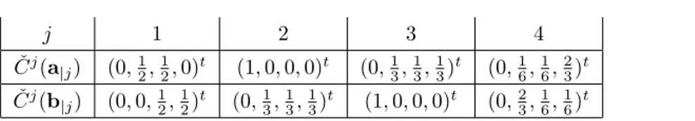
In Chapter 4, the class of Construct and Charge (CC -) rules for mcst sit-uations is introduced. CC -rules are defined starting from charge systems, and specify particular allocation protocols rooted on the Kruskal algorithm for com-puting an mcst. Furthermore, the chapter focuses on the class of Obligation rules for mcst situations. A characteristic of Obligation rules is that they assign to an mcst situation a vector of cost contributions which can be obtained as a product of a double stochastic matrix with the cost vector of edges in the optimal tree provided by the Kruskal algorithm. It is proved that special charge systems, called conservative, lead to a subclass of CC -rules that coincides with the class of Obligation rules. An interesting feature of such rules is that different feasible orderings of the edges lead to the same cost allocations. Properties of particular

(15)

Obligation rules, as the Potters value (P -value) and the Pτ_{-value introduced in}

Chapter 3, are also discussed. It turns out that the P -value equals the Equal Remaining Obligations (ERO) rule suggested by Jos Potters (which explains the name of the value) and which is studied first in Feltkamp et al. (1994). Fur-thermore, the P -value turns out to be the average of the Pτ_{-values. Sections}

4.2-4.4 and 4.7 are based on Moretti, Tijs, Branzei, Norde (2008); section 4.5 is based on Tijs, Branzei, Moretti, Norde (2006a); section 4.6 is based on Branzei, Moretti, Norde, Tijs (2004).

In Chapter 5, it is first demonstrated that Obligation rules are cost monotonic and induce also a pmas. Then, a new way to define the irreducible core (Bird (1976)) is presented, based on a non-Archimedean semimetric. The Bird core correspondence turns out to have interesting monotonicity and additivity prop-erties, and each stable cost monotonic allocation rule for mcst situations is a selection of the Bird core correspondence. Section 5.2 is based on Tijs, Branzei, Moretti, Norde (2006a); sections 5.3 and 5.4 are based on Tijs, Moretti, Branzei, Norde (2006b).

In Chapter 6 an axiomatic characterization of the P -value is provided, where cone-wise positive linearity of the P -value is a fundamental property and where the decomposition of an mcst situation into simple mcst situations plays a role. Using the additivity property an axiomatic characterization of the Bird core correspondence is also given. A value-theoretic interpretation of the Obligation rules using sharing values for cost games is also discussed. Section 6.2 is based on Branzei, Moretti, Norde, Tijs (2004); section 6.3 is based on Tijs, Moretti, Branzei, Norde (2006b); section 6.4 is based on Moretti, Tijs, Branzei, Norde (2005).

In Chapter 7 it is shown that, for variants of classical mcst games, a pmas does not necessarily exist. In particular, this chapter deals with monotonic mcst situations and directed mcst situations. Directed mcst situations of a special kind are studied, namely those which show up in considering the problem of connecting units (houses) in mountains with a purifier. For such problems an easy method is described to obtain an mcst. It turns out that the cores of the related cost allocation problems have a simple structure and each core element can be extended to a pmas and also to a bi-monotonic allocation scheme

(16)

(Branzei et al. (2001), Voorneveld et al. (2002)). Sections 7.2 and 7.3 are based on Norde, Moretti, Tijs (2004); section 7.4 is based on Moretti, Norde, Pham Do, Tijs (2002).

(17)

Chapter 2

Connection situations and

games

2.1 Minimum cost spanning tree (mcst)

situa-tions

An (undirected) graph is a pair < V, E >, where V is a set of vertices or nodes and E is a set of edges e of the form {i, j} with i, j ∈ V , i 6= j. The complete

graph on a set V of vertices is the graph < V, EV >, where EV = {{i, j}|i, j ∈

V and i 6= j}.

A path between i and j in a graph < V, E > is a sequence of nodes (i0, i1, . . . ,

ik), where i = i0 and j = ik, k ≥ 1, such that {is, is+1} ∈ E for each s ∈

{0, ..., k − 1} and such that all these edges are distinct. A cycle in < V, E > is a

path from i to i for some i ∈ V . A path (i0, i1, . . . , ik) is without cycles if there

do not exist a, b ∈ {0, 1, . . . , k}, a 6= b, such that ia = ib. Two nodes i, j ∈ V

are connected in < V, E > if i = j or if there exists a path between i and j in

E. A connected component of V in < V, E > is a maximal subset of V with the

property that any two nodes in this subset are connected in < V, E >.

This monograph deals with minimum cost spanning tree (mcst) situations,

i.e. situations where a set N = {1, . . . , n} of agents is willing to be connected as

(18)

cheap as possible to a source (i.e. a supplier of a service) denoted by 0, based on a given weight (or cost) system of connection. In the sequel we use also the notation N0_{= N ∪ {0}, and w for the weight function, i.e. a map which assigns}

to each edge e ∈ EN0 a non-negative number w(e) representing the weight or

cost of edge e.

We denote an mcst situation with set of users N , source 0, and weight function w by < N0_{, w > (or simply w). Further, we denote by W}N0

the set of all mcst situations < N0_{, w > (or w) with node set N}0_{. For each S ⊆ N ,}

one can consider the mcst subsituation < S0_{, w}

|S0 >, where S0 = S ∪ {0} and

w|S0 : E_S0 → IR₊ is the restriction of the weight function w to E_S0 ⊆ E_N0,

i.e. w|S0(e) = w(e) for each e ∈ E_S0. If w(e) ∈ {0, 1} for every e ∈ E_N0,

the weight function w is called a simple weight function, and we refer then to

< N0_{, E}

N0, w > as a simple mcst situation.

Let < N0_{, w > be an mcst situation. The carrier Ca(w) of w is the set of}

edges with positive costs, i.e. Ca(w) = {e ∈ E : w(e) > 0}. Two nodes i and j are called (w, N0_{)-connected if i = j or if there exists a path (i}

0, . . . , ik) from i

to j, with w({is, is+1}) = 0 for every s ∈ {0, . . . , k − 1}. A (w, N0)-component of

N0_{is a maximal subset of N}0_{with the property that any two nodes in this subset}

are (w, N0_{)-connected. We denote by C}

i(w) the (w, N0)-component to which i

belongs and by C(w) the set of all the (w, N0_{)-components of N}0_{. Clearly, the}

collection of (w, N0_{)-components forms a partition of N}0_.

The cost of a network Γ ⊆ EN0 is w(Γ) =

P

e∈Γw(e). A network Γ is a

spanning network on S0 _{⊆ N}0 _{if for every e ∈ Γ we have e ∈ E}

S0 and for every

i ∈ S there is a path in < S0_{, Γ > from i to the source. For any mcst situation}

w ∈ WN0

it is possible to determine at least one spanning tree on N0_{, i.e. a}

spanning network without cycles on N0_{, of minimum cost; each spanning tree of}

minimum cost is called an mcst for N0 _{in w or, shorter, an mcst for w. Given a}

spanning network Γ on N0 _{we define the set of edges of Γ with nodes in S}0_{⊆ N}0

as the set EΓ

S0 = {{i, j}|{i, j} ∈ Γ and i, j ∈ S0}.

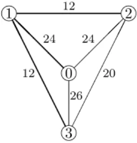
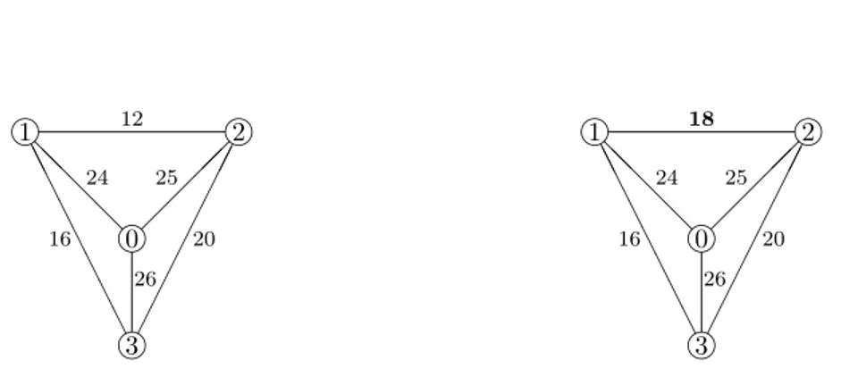
Example 2.1.1 In this example we consider a minimum cost spanning tree situation arising from the problem of car pooling. Suppose that three employees of a firm consider the possibility of car pooling in order to reduce their daily travel cost. The cost of driving a car from one employee to another or from one

(19)

employee to the firm are given in Figure 2.1. Here the employees are denoted @ @ @ @ A A A A A A A A ¢¢ ¢¢ ¢¢ ¢¢ ¡¡ ¡¡ i i i i 0 1 2 3 12 20 26 24 24 12 @ @ @ @ A A A A A A A A i i i i 0 1 2 3

Figure 2.1: An mcst situation < {0, 1, 2, 3}, w > (left side) and a related mcst (right side).

by 1, 2, and 3 and the firm by 0. To each edge e ∈ E{0,1,2,3} is assigned a

non-negative number w(e) representing the cost of edge e. A minimum cost spanning tree in this mcst situation < {0, 1, 2, 3}, w > is the network Γ =

{{0, 1}, {1, 2}, {1, 3}} with cost w(Γ) = 48. This network Γ corresponds to the

plan of car pooling in which employees 2 and 3 drive their car in solitude to employee 1 where all employees take one car in order to drive together to the firm. In the remaining of the thesis, to capture the attention of the reader on a certain mcst, we will represent the edges of the mcst by means of thicker lines, as it has been shown in Figure 2.2.

2.1.1 Algorithms for the determination of an mcst

Two famous algorithms for the determination of a minimum cost spanning tree are the algorithm of Prim (Prim (1957)) and the algorithm of Kruskal (Kruskal (1956)). Let < N0_{, w > be an mcst situation. A minimum cost spanning tree}

(20)

@ @ @ @ A A A A A A A A ¢¢ ¢¢ ¢¢ ¢¢ ¡¡ ¡¡ i i i i 0 1 2 3 12 20 26 24 24 12

Figure 2.2: An mcst situation < {0, 1, 2, 3}, w > and an mcst in <

{0, 1, 2, 3}, w > with edges denoted by thicker lines.

Prim’s Algorithm: In the first step construct an edge of minimal cost between a node in N and the source 0. In every subsequent step construct an edge of minimal cost between a node in N which is not connected yet with the source, directly or indirectly, and the source or with a node in N which is already connected with the source, directly or indirectly. In every step of the algorithm there is precisely one node in S which gets a connection with the source, so the algorithm stops after precisely |N | steps.

Kruskal’s Algorithm: In the first step construct an edge between nodes in N ∪{0} of minimal cost. In every subsequent step construct an edge between nodes in N ∪ {0} of minimal cost which does not form a cycle with the edges which have already been constructed. The algorithm also stops after precisely |N | steps.

Example 2.1.2 Consider the mcst situation < N0_{, w > of Example 2.1.1, with}

N0_{= {0, 1, 2, 3} and w as depicted in Figure 2.1.}

Prim’s Algorithm may first form edge {0, 1}, then {1, 2} (alternatively, {1, 3}), and finally {1, 3} (alternatively, {1, 2}). Having selected the edge {0, 1} in the first step, Prim’s algorithm on this mcst situation determines the mcst {{0, 1},

{1, 2}, {1, 3}}. On the same mcst situation, Prim’s Algorithm may first form

edge {0, 2}, then {1, 2}, and finally {1, 3}, bringing to the mcst {{0, 2}, {1, 2},

(21)

Kruskal’s Algorithm first forms the cheapest edge {1, 2} (alternatively, {1, 3}), then {1, 3} (alternatively, {1, 2}). After the first two steps of the Kruskal’s Al-gorithm, the cheapest edges {1, 2} and {1, 3} have been formed. Since edge

{2, 3} forms a cycle with the edges {1, 2} and {1, 3}, it cannot be constructed.

Finally, at the third step of the algorithm, one of the edges {0, 1} and {0, 2} may be formed. Depending on whether {0, 1} or {0, 2} is formed, the Kruskal’s Algorithm determines the mcst {{0, 1}, {1, 2}, {1, 3}} or {{0, 2}, {1, 2}, {1, 3}}, respectively.

2.1.2 Kruskal cones

The basic idea behind Kruskal’s algorithm is to consider edges one by one ac-cording to non-decreasing cost. This idea leads to the classification of mcst situations on the basis of the orders of the edges considered in Kruskal’s algo-rithm.

We define the set ΣE_{N 0} of linear orders on EN0 as the set of all bijections

σ : {1, . . . , |EN0|} → E_N0, where |E_N0| is the cardinality of the set E_N0. For each

mcst situation < N0_{, w > there exists at least one linear order σ ∈ Σ}

EN 0 such

that w(σ(1)) ≤ w(σ(2)) ≤ . . . ≤ w(σ(|EN0|)). We denote by wσ the column

vector¡w(σ(1)), w(σ(2)), . . . , w(σ(|EN0|))

¢t

. For any σ ∈ ΣEN 0 we define the set

Kσ = {w ∈ IREN 0

+ | w(σ(1)) ≤ w(σ(2)) ≤ . . . ≤ w(σ(|EN0|))}.

The set Kσ _{is a cone in IR}EN 0

+ , which we call the Kruskal cone with respect to

σ. One can easily see thatS_σ∈Σ

EN0K

σ_{= IR}EN 0

+ . For each σ ∈ ΣEN 0 the cone

Kσ _{is a simplicial cone with generators e}σ,k_{∈ K}σ_{, k ∈ {1, 2, . . . , |E}

N0|}, where

eσ,1_{(σ(j)) = 1 for all j ∈ {1, 2, . . . , |E}

N0|}, and for each k ∈ {2, . . . , |E_N0|}

eσ,k_{(σ(1)) = e}σ,k_{(σ(2)) = . . . = e}σ,k_{(σ(k − 1)) = 0}

and

eσ,k_{(σ(k)) = e}σ,k_{(σ(k + 1)) = . . . = e}σ,k_(σ(|E

N0|)) = 1.

(22)

This implies that each w ∈ Kσ_{can be written in a unique way as a non-negative}

linear combination of these generators. To be more concrete, for w ∈ Kσ _we

have w = w(σ(1))eσ,1₊ |EXN 0| k=2 ¡ w(σ(k)) − w(σ(k − 1))¢eσ,k_. _(2.2)

Clearly, we can also write WN0

=S_σ∈Σ

EN0K

σ_{, if we identify an mcst}

situ-ation < N0_{, w > with w.}

Let w ∈ WN0

and let σ ∈ ΣEN 0 be such that w ∈ K

σ_{. We can}

con-sider a sequence of precisely |EN0| + 1 graphs < N0, Fσ,0>, < N0, Fσ,1 >, . . . ,

< N0_{, F}σ,|EN 0| > such that Fσ,0 = ∅, Fσ,k = Fσ,k−1∪ {σ(k)} for each k ∈

{1, . . . , |EN0|}. For each graph < N0, Fσ,k >, with k ∈ {0, 1, . . . , |E_N0|}, let

πσ,k _{be the partition of N}0 _{consisting of the connected components of N}0 _in

< N0_{, F}σ,k_>.

Remark 2.1.1 For each k ∈ {1, . . . , |EN0|}, πσ,k is either equal to πσ,k−1 or is

obtained from πσ,k−1 _{by forming the union of two elements of π}σ,k−1_.

Now, we define recursively the function ρσ _{: {0, 1, . . . , |N |} → {0, 1, . . . , |E} N0|} by • ρσ_{(0) = 0} • ρσ_{(j) = min{k ∈ {ρ}σ_{(j − 1) + 1, . . . , |E} N0|}|πσ,k6= πσ,ρ σ_(j−1) } for each j ∈ {1, . . . , |N |}. Note that πσ,ρσ_(i)

6= πσ,ρσ_(j)

for each i, j ∈ {0, 1, . . . , |N |} with i 6= j, and

σ(ρσ_{(1)), . . . , σ(ρ}σ_{(|N |)) correspond to the |N | formed edges in the Kruskal’s}

algorithm when the order σ of the edges is considered.

Example 2.1.3 Consider the mcst situation < N0_{, w > with N}0 _{= {0, 1, 2, 3}}

and w as depicted in Figure 2.1. Note that w ∈ Kσ_{, with σ(1) = {1, 3},}

σ(2) = {1, 2}, σ(3) = {2, 3}, σ(4) = {0, 1}, σ(5) = {0, 2}, σ(6) = {0, 3}.

(23)

partitions πσ,k _{are shown in the following table} k Fσ,k _πσ,k 0 {∅} {{0}, {1}, {2}, {3}} 1 {{1, 3}} {{0}, {1, 3}, {2}} 2 {{1, 3}, {1, 2}} {{0}, {1, 2, 3}} 3 {{1, 3}, {1, 2}, {2, 3}} {{0}, {1, 2, 3}} 4 {{1, 3}, {1, 2}, {2, 3}, {0, 1}} {N0_} 5 {{1, 3}, {1, 2}, {2, 3}, {0, 1}, {0, 2}} {N0_} 6 {{1, 3}, {1, 2}, {2, 3}, {0, 1}, {0, 2}, {0, 3}} {N0_} Then, ρσ_{(0) = 0, ρ}σ_{(1) = 1, ρ}σ_{(2) = 2, ρ}σ_{(3) = 4.}

2.2 Cooperative game theory and mcst games

Next, we recall some basic game theoretical notions. A cooperative cost game or cost game is a pair (N, c), where N denotes the finite set of players and

c : 2N _{→ IR is the characteristic function, with c(∅) = 0 (here 2}N _denotes

the power set of player set N ). Often we identify a cost game (N, c) with the corresponding characteristic function c. A group of players T ⊆ N is called a

coalition and c(T ) is called the cost of this coalition. The class of all cost games

with N as set of players is denoted by GN_{. Let H}N _{⊆ G}N_{. We call a map}

ψ : HN _{→ IR}N _{a value if it assigns to every cost game (N, c) ∈ H}N _{one payoff}

vector (or cost allocation) in IRN_{. A payoff vector x ∈ IR}N _{is efficient for a cost}

game (N, c) ∈ GN _{if we have}P

i∈Nxi= c(N ). A value ψ is efficient if we have

that ψ(c) is an efficient payoff vector for each c ∈ HN_{. A value ψ : H}N _{→ IR}N

is called linear if ψ(βv + γu) = βψ(v) + γψ(u) for all games v, u ∈ HN _{and real}

numbers β, γ ∈ IR such that βv + γu ∈ HN_.

A particular set, possibly empty, of payoff vectors of a cost game (N, c) is the

core, which is defined as the set of efficient payoff vectors for which no coalition

has an incentive to leave the grand coalition N . In formula

core(c) = {x ∈ IRN_|X i∈S xi≤ c(S) ∀S ∈ 2N \ {∅}; X i∈N xi = c(N )}.

(24)

A game (N, c) is called a concave game if the marginal contribution of any player to any coalition is not less than his marginal contribution to a larger coalition,

i.e. if it holds that

c(S ∪ {i}) − c(S) ≥ c(T ∪ {i}) − c(T ) (2.3)

for all i ∈ N and all S ⊆ T ⊆ N \ {i}.

We define the set ΣN of possible orders on the set N as the set of all bijections

τ : {1, . . . , |N |} → N , where |N | is the cardinality of the set N and where τ (i) = j means that with respect to τ , player j is in the i-th position.

Let (N, c) be a cooperative cost game. For τ ∈ ΣN, the marginal vector

mτ_{(c) is defined by}

mτi(c) = c([i, τ ]) − c((i, τ )) for all i ∈ N,

where [i, τ ] = {j ∈ N : τ−1_{(j) ≤ τ}−1_{(i)} is the set of predecessors of i with}

respect to τ including i, and (i, τ ) = {j ∈ N : τ−1_{(j) < τ}−1_{(i)} is the set of}

predecessors of i with respect to τ excluding i. In a coherent way with respect to previous notations, we will indicate the set [i, τ ] ∪ {0} and (i, τ ) ∪ {0} as [i, τ ]0 _{and (i, τ )}0_{, respectively. For instance, for each k ∈ {1, . . . , |N |} and for}

each l ∈ {2, . . . , |N |}, the set [τ (k), τ ]0 _{= {0, τ (1), . . . , τ (k)} and (τ (l), τ )}0 ₌

{0, τ (1), . . . , τ (l − 1)}, which will be denoted shorter as [τ (k)]0 _{and (τ (l))}0_,

re-spectively.

The most well-known value in the theory of cost games is the Shapley value (Shapley (1953)). The Shapley value φ(c) of a cost game (N, c) is defined as the average of marginal vectors over all |N |! possible orders in ΣN. In formula

φi(c) = X τ ∈ΣN mτ i(c) |N |! for all i ∈ N. (2.4)

A population monotonic allocation scheme or pmas (Sprumont (1990)) of the game (N, c) is a scheme x = {xS,i}S∈2N_\{∅},i∈S with the properties

i) X

i∈S

xS,i= c(S) for all S ∈ 2N\{∅};

(25)

A pmas provides a cost allocation vector for every coalition in a monotonic way, i.e. the cost allocated to some player decreases if the coalition to which he belongs becomes larger.

Let < N0_{, w > be an mcst situation. The minimum cost spanning tree game}

(N, cw) (or simply cw), corresponding to < N0, w >, is defined by

cw(S) = min{w(Γ)|Γ is a spanning network on S0}

for every S ∈ 2N_{\{∅}, with the convention that c}

w(∅) = 0.

We denote by MCSTN _{the class of all mcst games corresponding to mcst}

situations in WN0

. For each σ ∈ ΣEN 0, we denote by G

σ _{the set {c}

w | w ∈

Kσ_{} which is a cone. We can express MCST}N _{as the union of all cones G}σ_,

i.e. MCSTN = S_σ∈Σ

EN0G

σ_{, and we would like to point out that MCST}N

itself is not a cone if |N | ≥ 2.

Example 2.2.1 Consider the mcst situation < N0_{, w > with N}0 _{= {0, 1, 2, 3}}

and w as depicted in Figure 2.1.

If S = {1, 2} then a minimum cost spanning network for S is Γ = {{1, 2},

{0, 1}} with cost 36, whereas the minimum cost spanning network for S = {3}

is Γ = {{0, 3}} with cost 26. Proceeding in this way we find that the mcst game (N, cw), corresponding to < N0, w >, is given by

cw(123) = 48,

cw(12) = 36, cw(13) = 36, cw(23) = 44,

cw(1) = 24, cw(2) = 24, cw(3) = 26.

We call a map F : WN0

→ IRN _{assigning to every mcst situation w a unique cost}

allocation in IRN _{a solution. A solution F is efficient if we have}P

i∈NFi(w) =

w(Γ) for each w ∈ WN0

, where Γ is a spanning network on N0 _{of minimal cost.}

A solution F has the carrier property if Fi(w) = 0 for each w ∈ WN

0

and for each i ∈ N such that i is (w, N0_{)-connected to 0.}

The core C(cw) of an mcst game cw ∈ MCSTN is nonempty (Granot and

Huberman (1981), Bird (1976)) and, given an mcst Γ (with no cycles) for N0

in the mcst situation w, one can easily find an element in the core looking at the algorithm of Prim described in Section 2.1.1. If one assigns the cost of an

(26)

edge, which is formed in some step of the algorithm, to the player who just gets a connection with the source, directly or indirectly, then one obtains a core ele-ment of the corresponding mcst game (see Bird (1976) for more details). In the following example we will illustrate that such a procedure does not necessarily generate a pmas of the corresponding mcst game.

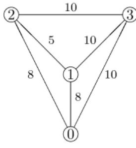
Example 2.2.2 Consider the complete weighted graph < N0_{, ˜}_{w > with N}0 ₌

{0, 1, 2, 3} and cost function ˜w as depicted in Figure 2.3. Application of Prim’s

¡¡ ¡¡ @ @ @ @ ¢¢ ¢¢ ¢¢ ¢¢ A A A A A A A A i i i i 0 1 2 3 13 8 18 6 17 21

Figure 2.3: The cost function ˜w on E{0,1,2,3}.

algorithm for the mcst situation < {0, 1, 2, 3}, ˜w > yields the formation of edge {0, 1} first, followed by the formation of edge {1, 3} and edge {2, 3}. The cost

of edge {0, 1} is assigned to player 1, the cost of edge {1, 3} to player 3 and the cost of edge {2, 3} to player 2. Following the same procedure for all other coalitions we get the following table

S 1 2 3 {1, 2, 3} 6 8 13 {1, 2} 6 17 ∗ {1, 3} 6 ∗ 13 {2, 3} ∗ 17 8 {1} 6 ∗ ∗ {2} ∗ 17 ∗ {3} ∗ ∗ 18

This table does not provide a pmas of the corresponding mcst game ({1, 2, 3},

cw˜): in coalition S = {2, 3} player 3 has to pay 8 which is strictly less than the

(27)

(28)

(29)

Chapter 3

Mcst games and population

monotonic allocation

schemes

3.1 Introduction

In Example 2.2.2 it has been provided an mcst situation where the allocation method introduced by Bird (1976) does not generate a pmas of the correspond-ing mcst game. But it is not clear, up to this point of the story, whether it is possible to find a solution for mcst situations which is always able to generate a pmas. Solving this problem is particularly valuable in applications where the cardinality of the set of agents can vary in time.

Consider for instance the mcst situation introduced in Example 2.1.1. Prim’s Algorithm may first form edge {0, 1} at the first step, then {1, 2}, and finally

{1, 3} and the Bird rule yields the core allocation x = (24, 12, 12).

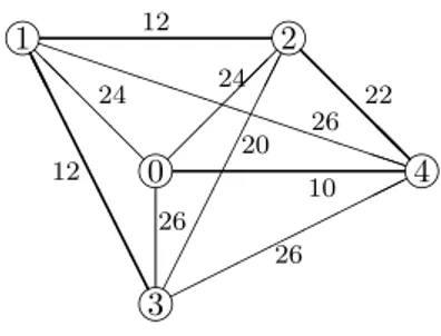
Suppose now that a fourth employee is asking whether he can join the car-poolers 1, 2, and 3. The cost of driving from employee 4 to the other employees and to the firm are given in Figure 3.1, as well as a minimum spanning tree for the new situation. Application of the Bird rule to this new situation yields the

(30)

A A A A A A A A @ @ @_@ ©©©© ©©©© PPP PPP PPP_PP P @ @ @ @ ¢¢ ¢¢ ¢¢ ¢¢ ¡¡ ¡¡ i i i i i 0 1 2 3 4 12 20 26 24 24 12 26 22 26 10

Figure 3.1: The cost of driving and a minimum spanning tree in the new situa-tion.

allocation x = (12, 22, 12, 10). In the new situation employee 2 has to pay 22, whereas in the old situation he only paid 12. Therefore, if the employees use the Bird rule in order to divide joint costs, employee 2 will veto the entrance of employee 4. Note that if Prim’s Algorithm applied to the mcst situation in Example 2.1.1 would have formed edge {0, 2} at the first step, then {1, 2}, and finally {1, 3}, bringing to the mcst {{0, 2}, {1, 2}, {1, 3}}, the Bird rule would have provided the allocation (12, 24, 12). With respect to this allocation in the mcst situation of Figure 2.1, according to the Bird rule in the new mcst situation of Figure 3.1, no employees would have put a veto on the entrance of employee 4.

The central question in this chapter is whether every minimum cost span-ning tree game has a population monotonic allocation scheme (pmas) (Sprumont (1990)), which is an allocation scheme that provides a core element for the game and all its subgames and which, moreover, satisfies a monotonicity condition in the sense that players have to pay less in larger coalitions. We will answer this question in the affirmative and we will provide the Subtraction Algorithm, that computes for every minimum cost spanning tree game a pmas. We will show that this algorithm is closely related to Kruskal’s algorithm for finding a minimum spanning tree (Kruskal (1956)). The Subtraction Algorithm is based upon a decomposition theorem, which shows that every minimum cost spanning tree game can be written as a non-negative combination of minimum cost spanning tree games corresponding to simple mcst situations.

(31)

theo-rem is provided and minimum cost spanning tree games corresponding to simple mcst situations are studied. The Subtraction Algorithm is presented in Section 3.3. This chapter is based on Norde, Moretti, Tijs (2004).

3.2 Simple mcst games and the decomposition

theorem

If the cost of all edges in Ca(w) are lowered by the cost of an edge in Ca(w) with minimal cost we are left with a cost function with smaller carrier. The following lemma establishes a relation between the corresponding mcst games. Lemma 3.2.1 Let w ∈ WN0

be a cost function with Ca(w) 6= ∅ and let α :=

min{w(l) : l ∈ Ca(w)}. Let w0 _{be the simple cost function defined by w}0_{(l) := 1}

if l ∈ Ca(w) and w0_{(l) := 0 otherwise. Let w}00 _{be the cost function defined by}

w00_{(l) := w(l) − αw}0_{(l) for every l ∈ E}

N0. Finally, let c, c0 and c00 be the mcst

games corresponding to w, w0 _{and w}00_{respectively. Then, we have w = αw}0_+w00

and c = αc0_{+ c}00_.

Proof It follows by definition that w = αw0 _{+ w}00_{. In order to prove that}

c = αc0_{+ c}00_{, i.e. c(S) = αc}0_{(S) + c}00_{(S) for every S ∈ 2}N_{\{∅}, let S ∈ 2}N_\{∅}.

Let Γ0 _{be a minimum cost spanning network for S in w}0_{without cycles, i.e. Γ}0 _is

a minimum cost spanning tree for S in w0_{. Write Γ}0_{= L}0_{∪ L}1_{where L}0_{:= {l ∈}

Γ0_{: w}0_{(l) = 0} and L}1_{:= {l ∈ Γ}0 _{: w}0_{(l) = 1}. Clearly, |Γ}0_{| = |L}0_{| + |L}1_{|. Since}

Γ0 _{is a tree we also have |Γ}0_{| = |S|. Hence, c}0_{(S) = w}0_(Γ0_{) = |L}1_{| = |S| − |L}0_|.

It suffices to show that there exists a minimum cost spanning tree Γ00 _{for S}

in w00 _{with L}0 _{⊆ Γ}00_{. Since then Γ}00 _{contains at most |Γ}00_\L0_{| = |S| − |L}0_|

edges in Ca(w0_{) and hence w}0_(Γ00_{) ≤ |S| − |L}0_{| = w}0_(Γ0_{). Therefore, Γ}00 _is

also a minimum cost spanning tree for S in w0_{. Having w = αw}0_{+ w}00 _and

the fact that Γ00 _{is a minimum cost spanning tree for S in both w}0 _{and w}00 _we

may conclude that Γ00 _{is also a minimum cost spanning tree for S in w. So,}

c(S) = w(Γ00_{) = αw}0_(Γ00_{) + w}00_(Γ00_{) = αc}0_{(S) + c}00_(S).

In order to show that there is a minimum cost spanning tree Γ00 _{for S in w}00

with L0 _{⊆ Γ}00 _{take an arbitrary minimum cost spanning tree Γ for S in w}00_.

(32)

contains a cycle C, whereas Γ0_{, and hence L}0_{, do not contain cycles, we can find}

an edge l0 _{∈ C with l}0 _{∈ L}_/ 0_{. Define ˜}_{Γ := (Γ ∪ {l})\{l}0_{}. Since w}00_{(l) = 0 and}

w00_(l0_{) ≥ 0 we find that also ˜}_{Γ is a minimum cost spanning tree for S in w}00_.

Moreover |˜Γ ∩ L0_{| = |Γ ∩ L}0_{| + 1. Repeating this argument results in the tree}

Γ00 _{with the desired properties.}

The following decomposition theorem shows that every minimum cost span-ning tree game can be written as a non-negative combination of minimum cost spanning tree games corresponding to simple mcst situations.

Theorem 3.2.2 Let w ∈ WN0

be a cost function with Ca(w) 6= ∅ and let c be the corresponding mcst game. Then, there exists a sequence of simple cost functions w1, . . . , wk, with Ca(w) = Ca(w1) ⊃ Ca(w2) ⊃ · · · ⊃ Ca(wk), and

positive numbers α1, . . . , αk such that

w =

k

X

j=1

αjwj. (3.1)

Moreover, if c1, . . . , ck are the mcst games corresponding to w1, . . . , wk

respec-tively, we have c = k X j=1 αjcj. (3.2)

Proof The proof is by induction to |Ca(w)|.

If |Ca(w)| = 1 then Ca(w) has a unique element, say l∗_{. Defining α := w(l}∗₎

and the simple cost function w1 by w1(l∗) := 1 and w1(l) := 0 if l 6= l∗ we

clearly have w = α1w1. Moreover, if c1 is the mcst game corresponding to w1

one easily verifies that c = α1c1.

Now, let m ∈ IN, m ≥ 2 and suppose that the assertion has been proved for every cost function w with |Ca(w)| ≤ m − 1. Consider a cost function w with

|Ca(w)| = m. According to Lemma 3.2.1 there is a simple cost function w1,

namely the simple cost function with the same carrier as w, a positive number

α1 and a cost function w00 with Ca(w00) ⊂ Ca(w) such that w = α1w1 +

w00_{. Moreover, if c}

1 and c00 are the mcst games corresponding to w1 and w00

respectively, we have c = α1c1+ c00. Application of the induction hypothesis to

(33)

Remark 3.2.1 In order to prove relation (3.1), one may directly observe that

WN0

=S_σ∈Σ

EN0K

σ_{, where K}σ_{is the Kruskal cone with respect to σ, σ ∈ Σ} EN 0,

introduced in Section 2.1.2. As we already remarked in relation (2.2), w ∈ Kσ

can be written in a unique way as a non-negative linear combination of the generators of the simplicial cone Kσ_.

Example 3.2.1 Consider the cost function w of Example 2.1.1. Note that

w ∈ Kσ_{, with σ(1) = {1, 3}, σ(2) = {1, 2}, σ(3) = {2, 3}, σ(4) = {0, 1},}

σ(5) = {0, 2}, σ(6) = {0, 3}. Hence, by relation (2.2), we have w = w(σ(1))eσ,1₊P|EN 0|

k=2

¡

w(σ(k)) − w(σ(k − 1))¢eσ,k

= 12eσ,1_{+ (12 − 12)e}σ,2_{+ (20 − 12)e}σ,3

+(24 − 20)eσ,4_{+ (24 − 24)e}σ,5_{+ (26 − 24)e}σ,6₌

= 12eσ,1_{+ 8e}σ,3_{+ 4e}σ,4_{+ 2e}σ,6_.

In terms of Theorem 3.2.2 we may write

w = α1w1+ α2w2+ α3w3+ α4w4

where α1 = 12, α2 = 8, α3 = 4 and α4 = 2, and the simple cost functions

w1, . . . , w4 are specified by edge l {1, 3} {1, 2} {2, 3} {0, 1} {0, 2} {0, 3} w1(l) = eσ,1(l) 1 1 1 1 1 1 w2(l) = eσ,3(l) 0 0 1 1 1 1 w3(l) = eσ,4(l) 0 0 0 1 1 1 w4(l) = eσ,6(l) 0 0 0 0 0 1

Computing the mcst games c1, . . . , c4 corresponding to w1, . . . , w4respectively,

we get coalition S {1} {2} {3} {1,2} {1,3} {2,3} {1,2,3} c1(S) 1 1 1 2 2 2 3 c2(S) 1 1 1 1 1 2 1 c3(S) 1 1 1 1 1 1 1 c4(S) 0 0 1 0 0 0 0

(34)

One easily verifies thatP4_i=1αicicoincides with the mcst game c, as computed

in Example 2.2.1.

3.3 The Subtraction Algorithm for population

monotonic allocation scheme (pmas)’s

gen-eration

In this section we will focus on simple cost functions. We show that an mcst game corresponding to a simple cost function has a population monotonic allo-cation scheme. Using Theorem 3.2.2 we obtain as a corollary that every mcst game has a population monotonic allocation scheme.

Let w be a simple cost function and let S ∈ 2N_{\{∅} be a coalition. Two}

nodes i and j in S ∪ {0} are (w, S0_{)-connected if there exists a sequence of nodes}

i = i0, . . . , ik = j in S ∪ {0} with w({is, is+1}) = 0 for every s ∈ {0, . . . , k − 1}.

A (w, S0_{)-component of S ∪ {0} is a maximal subset of S ∪ {0} with the property}

that any two nodes in this subset are (w, S0_{)-connected. The number of (w, S}0

)-components is denoted by n(w, S0_{). Clearly, the collection of (w, S}0_)-components

forms a partition of S ∪ {0}.

Lemma 3.3.1 Let w be a simple cost function and let c be the corresponding

mcst game. Then, we have

c(S) = n(w, S0_{) − 1}

for every S ∈ 2N_\{∅}.

Proof Let S ∈ 2N_{\{∅}. If n(w, S}0_{) = 1 then S ∪ {0} is the unique (w, S}0

)-component. Therefore, Γ = {l ∈ EN0 : l ⊆ S ∪ {0}, w(l) = 0} is a spanning

network for S with w(Γ) = 0. Hence, c(S) = 0 = n(w, S0_{) − 1.}

Now, suppose n(w, S0_{) ≥ 2. Let C}

0, C1, . . . , Ck (k ≥ 1) be all (w, S0

)-compo-nents. Clearly, S∪{0} = ∪k

(35)

we may assume that 0 ∈ C0. For every i ∈ {1, . . . , k} select some node ni∈ Ci.

Consider the network

Γ = {l ∈ EN0 : l ⊆ S ∪ {0}, w(l) = 0} ∪ {{n_i, 0} : i ∈ {1, . . . , k}}.

The network Γ is a spanning network for S: nodes in C0 are connected with

source 0 via edges in Γ of zero cost, and nodes in Ci with i ∈ {1, . . . , k} are

connected with the source via node ni. Moreover w(Γ) = k. It suffices to

show that for any spanning tree Γ0 _{for S we have w(Γ}0_{) ≥ k, since then Γ}

is a minimum cost spanning network for S in w, and hence we have c(S) =

w(Γ) = k = n(w, S0_{) − 1. So, let Γ}0 _{be a spanning tree for S. Define, for every}

i ∈ {0, . . . , k}, Γi:= Γ0∩ {l ∈ EN0 : l ⊆ C_i, w(l) = 0}. Since Γ0, and hence Γ_i,

does not contain cycles we have |Γi| ≤ |Ci| − 1 for every i ∈ {0, . . . , k}. Write

Γ0 _{= L}0_{∪ L}1 _{where L}0 _{:= {l ∈ Γ}0 _{: w(l) = 0} and L}1 _{:= {l ∈ Γ}0 _{: w(l) = 1}.} Since L0_{⊆ ∪}k i=0Γi we have |L0_{| ≤} k X i=0 |Γi| ≤ k X i=0 |Ci| − (k + 1) = |S| + 1 − (k + 1) = |S| − k. Therefore, w(Γ0_{) = |L}1_{| = |Γ}0_{| − |L}0_{| = |S| − |L}0_{| ≥ k.}

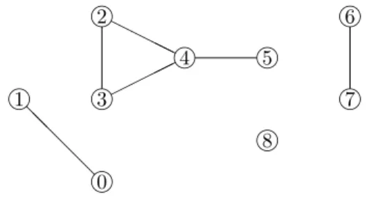
Example 3.3.1 Consider the complete weighted graph < N0_{, w > with N}0 ₌

{0, . . . , 8} and simple cost function w specified by {l ∈ EN0 : w(l) = 0} =

{{0, 1}, {2, 3}, {2, 4}, {3, 4}, {4, 5}, {6, 7}}. Let c be the corresponding mcst game.

The edges with zero cost are depicted in Figure 3.2. Clearly, {0, 1}, {2, 3, 4, 5},

{6, 7} and {8} are all (w, N )-components. Consequently, c(N ) = n(w, N ) − 1 =

4 − 1 = 3. If we consider for example coalition S = {2, 3, 5, 6} we get that

{0}, {2, 3}, {5} and {6} are all (w, S0_{)-components. Consequently, we also have}

c(S) = n(w, S0_{) − 1 = 4 − 1 = 3.}

In order to show that an mcst game corresponding to a simple cost function has a pmas we need some more notation. In the following, if w ∈ WN0

is a simple cost function, S ∈ 2N_{\{∅} and i ∈ S then the (w, S}0_{)-component to which i}

(36)

Figure 3.2: The cost function of Example 3.3.1.

Definition 3.3.1 Let w ∈ WN0

be a simple cost function and let τ ∈ ΣN. The

scheme xτ,w_{= (x}τ,w

S,i)S∈2N_\{∅},i∈S is defined in the following way:

xτ,w_S,i =          0 if 0 ∈ Ci(w, S),

0 if 0 /∈ Ci(w, S) and τ−1(i) 6= min j∈Ci(w,S)

τ−1_(j),

1 if 0 /∈ Ci(w, S) and τ−1(i) = min j∈Ci(w,S)

τ−1(j), for every S ∈ 2N_{\{∅} and for every i ∈ S.}

The scheme xτ,w _{provides for every coalition S ∈ 2}N_{\{∅} a division of the cost}

c(S) in the following way: all members of the (w, S0_{)-component containing the}

source 0 do not have to pay anything whereas the (unit) cost of all other (w, S0

)-components is allocated to the member in the component with the lowest index according to τ .

Example 3.3.2 Consider the simple cost function w of Example 3.3.1 and let

τ ∈ ΣN be given by τ−1(1) = 2, τ−1(2) = 7, τ−1(3) = 5, τ−1(4) = 3, τ−1(5) =

6, τ−1_{(6) = 8, τ}−1_{(7) = 1 and τ}−1_{(8) = 4. Then, x}τ,w

N,1= xτ,wN,2 = xτ,wN,3= xτ,wN,5=

xτ,w_N,6 = 0 and xτ,w_N,4 = xτ,w_N,7 = xτ,w_N,8 = 1. Moreover, for S = {2, 3, 5, 6} we get

xτ,w_S,2 = 0 and xτ,w_S,3 = xτ,w_S,5 = xτ,w_S,6 = 1.

In the following lemma we prove that the scheme xτ,w _{is a pmas for the mcst}

game corresponding to simple cost function w.

Lemma 3.3.2 Let w be a simple cost function, cwthe corresponding mcst game,

(37)

Proof Let S ∈ 2N_{\{∅}. Every (w, S}0_{)-component which does not contain the}

source 0 contains precisely one player i ∈ S with xτ,w_S,i = 1. Therefore, X

i∈S

xτ,w_S,i = n(w, S0_{) − 1 = c(S).}

Now, let i ∈ N and S, T ∈ 2N_{\{∅} be such that i ∈ S ⊂ T . In order to show}

that xτ,w_S,i ≥ xτ,w_T,i it suffices to show that xτ,w_T,i = 1 implies xτ,w_S,i = 1. So, assume

xτ,w_T,i = 1, i.e. 0 6∈ Ci(w, T ) and

τ−1(i) = min

j∈Ci(w,T )

τ−1(j).

Obviously, we have Ci(w, S) ⊆ Ci(w, T ), which implies 0 6∈ Ci(w, S) and

τ−1_{(i) =} _min j∈Ci(w,S)

τ−1_(j).

Therefore, xτ,w_S,i = 1.

As a corollary we get the main theorem of this section. Theorem 3.3.3 Every mcst game has a pmas.

Proof The theorem follows directly from Theorem 3.2.2, Lemma 3.3.2 and the observation that if x1 _{= (x}1

S,i)S∈2N_\{∅},i∈S is a pmas for game c1 and

x2_{= (x}2

S,i)S∈2N_\{∅},i∈S is a pmas for game c2, then we have that αx1+ βx2:=

(αx1

S,i+ βx2S,i)S∈2N_\{∅},i∈S is a pmas for αc1+ βc2 for every α ≥ 0 and every

β ≥ 0.

A basis for an algorithm that finds a pmas in any mcst game is provided by The-orem 3.2.2 and Lemma 3.3.2. Let w ∈ WN0

with Ca(w) 6= ∅ and let σ ∈ ΣEN 0

be such that w ∈ Kσ_{. As we already remarked in relation (2.2), w ∈ K}σ_{can be}

written in a unique way as a non-negative linear combination of the generators of the simplicial cone Kσ_{, in formula}

w = w(σ(1))eσ,1₊ |EXN 0|

k=2

¡

w(σ(k)) − w(σ(k − 1))¢eσ,k_.

Note that Ca(eσ,1_{) ⊃ · · · ⊃ Ca(e}σ,k_{). Theorem 3.2.2 tells us that the same}

(38)

to w and eσ,1_{, . . . , e}σ,|EN 0|, respectively: cw= w(σ(1))c1+ |E_X_{N 0}| k=2 ¡ w(σ(k)) − w(σ(k − 1))¢ck.

Subsequently, fix some permutation τ ∈ ΣN. Compute, for every k ∈ {1, . . . ,

|EN0|}, the scheme xτ,e σ,k

. According to Lemma 3.3.2 the scheme xτ,eσ,k

is a pmas for ckfor every k ∈ {1, . . . , |EN0|}. Define the scheme Pτ,win the following

way: Pτ,w _{:= w(σ(1))x}τ,eσ,1 +P|EN 0| k=2 ¡ w(σ(k)) − w(σ(k − 1))¢xτ,eσ,k (3.3) or, alternatively, Pτ,w_:=³ P|EN 0|−1 k=1 ¡ xτ,eσ,k − xτ,eσ,k+1¢ w(σ(k)) ´

+ w(σ(|EN0|))xτ,eσ,|EN0 |.

(3.4) For the same arguments used to prove Theorem 3.3.3, we have that Pτ,w _{is a}

pmas for the mcst game cw. For the sake of completeness note that for w = 0

the vectors P_S,iτ,w := 0, for every S ∈ 2N_{\{∅} and each i ∈ S, determine a pmas}

for the corresponding minimum cost spanning tree game cw= 0.

Example 3.3.3 Consider the cost function w of Example 2.1.1 and the corre-sponding mcst game c introduced in Example 2.2.1. As we already noted in Example 2.1.3 and Example 3.2.1, we have that w ∈ Kσ_{, with σ(1) = {1, 3},}

σ(2) = {1, 2}, σ(3) = {2, 3}, σ(4) = {0, 1}, σ(5) = {0, 2}, σ(6) = {0, 3} and, by relation (2.2), w = w(σ(1))eσ,1₊P|EN 0| k=2 ¡ w(σ(k)) − w(σ(k − 1))¢eσ,k

= 12eσ,1_{+ (12 − 12)e}σ,2_{+ (20 − 12)e}σ,3

+(24 − 20)eσ,4_{+ (24 − 24)e}σ,5_{+ (26 − 24)e}σ,6₌

= 12eσ,1_{+ 8e}σ,3_{+ 4e}σ,4_{+ 2e}σ,6_.

(39)

that Pτ,w _{is given by the following sum}

Pτ,w_{= 12x}τ,eσ,1_{+ 8x}τ,eσ,3_{+ 4x}τ,eσ,4_{+ 2x}τ,eσ,6

= S 1 2 3 {1, 2, 3} 12 12 12 {1, 2} 12 12 ∗ {1, 3} 12 ∗ 12 {2, 3} ∗ 12 12 {1} 12 ∗ ∗ {2} ∗ 12 ∗ {3} ∗ ∗ 12 + S 1 2 3 {1, 2, 3} 8 0 0 {1, 2} 8 0 ∗ {1, 3} 8 ∗ 0 {2, 3} ∗ 8 8 {1} 8 ∗ ∗ {2} ∗ 8 ∗ {3} ∗ ∗ 8 + S 1 2 3 {1, 2, 3} 4 0 0 {1, 2} 4 0 ∗ {1, 3} 4 ∗ 0 {2, 3} ∗ 4 0 {1} 4 ∗ ∗ {2} ∗ 4 ∗ {3} ∗ ∗ 4 + S 1 2 3 {1, 2, 3} 0 0 0 {1, 2} 0 0 ∗ {1, 3} 0 ∗ 0 {2, 3} ∗ 0 0 {1} 0 ∗ ∗ {2} ∗ 0 ∗ {3} ∗ ∗ 2 = S 1 2 3 {1, 2, 3} 24 12 12 {1, 2} 24 12 ∗ {1, 3} 24 ∗ 12 {2, 3} ∗ 24 20 {1} 24 ∗ ∗ {2} ∗ 24 ∗ {3} ∗ ∗ 26