OATAO is an open access repository that collects the work of Toulouse
researchers and makes it freely available over the web where possible
Any correspondence concerning this service should be sent
to the repository administrator:
tech-oatao@listes-diff.inp-toulouse.fr
This is an author’s version published in:
http://oatao.univ-toulouse.fr/24156
To cite this version:
Hernandez Torres, David and Turpin, Christophe and
Roboam, Xavier and Sareni, Bruno Techno-economical
optimization of wind power production including lithium and/or
hydrogen sizing in the context of the day ahead market in
island grids. (2019) Mathematics and Computers in
Simulation, 158. 162-178. ISSN 0378-4754
Official URL:
https://doi.org/10.1016/j.matcom.2018.07.010
Techno-economical optimization of wind power production
including lithium and/or hydrogen sizing in the context of the day
ahead market in island grids
David Hernandez-Torres, Christophe Turpin, Xavier Roboam
*
, Bruno Sareni
Laboratoire Plasma el Co11versio11 d'E,iergie (LAPLACE), UMR5213-CNRS-INPT-UPS, Toulouse, France
Abstract
In this article an optimal storage sizing based on technical and economical modeling is presented. A focus is made on wind power producers participating in day-ahead markets for island networks and energy storage using Li-Ion and H2/02 batteries. The modeling approach is based on power flow models and detailed optimization-oriented techniques. An importance is given to the storage device ageing effects on the overall hybrid system levelized cost of the energy. The results are presented for the special case of renewable power integration in the French islands networks. The analysis obtained after the results shows the importance of this type of modeling tool for decision making during the initial conceptual design level.
Keywords: Wind power; Optimal storage sizing; Day-ahead markets; Island networks 1. Introduction
The massive integration of renewable energy sources (RES) in island networks is of great concem because of the absence of extended, robust and interconnected electric infrastructures. Mature and well established technologies, such as wind and solar power, are intermittent by nature, thus limiting the amount of installed power available from these sources in order to avoid stability problems. Energy storage systems (ESS) are a solution to cope with the intermittent character of renewable sources. They are used to efficiently smooth power output and to store exceeding or failing production. In the context of French island networks with high penetration rates of renewable energy already installed (e.g. Réunion and Guadeloupe islands), a limitation of 30% in renewable penetration rate has been imposed in order to preserve the electical grid stability. Storage devices with power management could then be used to increase the
r saturated renewable penetration ratio in these sites. * Corresponding author.
E-mail addresses: dhemandez@laplace.univ-tlse.fr (D. Hemândez-Torres), turpin@laplace.univ-tlse.fr (C. Turpin),
In this kind of system, the installation should be capable of managing in real-time, the produced power from the sources and the storage devices, in order to propose a good quality power delivery service. Under the condition of a storage device installation, the wind power producers are allowed to participate in forward markets, particularly in the day-ahead market, where the majority of today’s agreements of power delivery are made [5]. The energy management system of the hybrid plant should be able to guarantee the commitment imposed by the day-ahead planning in order to avoid penalties from the grid operator. This kind of restrictions imposes that the energy management strategies (EMSs) should be precise, but also that the storage system should be properly sized to guarantee the power commitment under uncertain stochastic power production from renewable sources. The problem of EMSs design has been broadly studied in the literature. The impact of optimal EMSs for maximizing the profit of a wind power producer is well presented in [5]. Other interesting optimal EMSs are presented in [24,23,16,9]. Some practical and efficient rule-based/heuristic EMSs with RES are also given in [15,14,4,8]. Intermediate studies considering both optimal control and sizing for RES integration to power networks are presented in [6] using linear programming and model predictive control and in [12] using dynamic programming and optimal control.
A similar modeling philosophy is used in [17] or even in [10]. However, the tools proposed in these works are proprietary and often not modifiable (new EMSs techniques or even different grid ancillary services are hard to implement). Some original and efficient heuristic EMSs for several RES and ESS types can be found in [14,4].
Other interesting optimal sizing approaches are developed in the literature, using constrained optimization on a simplified techno-economical model in [18], or using optimal cost minimization with a battery ageing model in [25]. Optimal sizing is also studied in electricity markets using special bidding planning strategies in [19] and with a risk hedging against penalties strategy in [21]. ESS sizing is also proposed based on the forecast data statistical information in [3]. The impact on storage sizing of the day-ahead forecast is presented in [11].
This article is focused on the modeling and optimal sizing of a system with ESS associated with RES using a techno-economic perspective. A simulation and optimization tool has been developed at LAPLACE laboratory in Toulouse to study this type of system. The modeling approach is oriented towards an optimal sizing of storage devices. It is then important to consider models that are valid in the scale of the system life span (i.e. several years). Following this modeling approach, a focus is given in this article to heuristic EMSs techniques. The main contribution of this article is the integration of an optimal sizing methodology for long simulation horizons, on the scale of the system life span, including the nonlinearities of the ESS by considering detailed optimization-oriented models of the ESS. Ageing and degradation models of the ESS are of special interest in this article.
This article is divided in three main sections. In the two first sections the system modeling and the energy management strategies are described. The last section is devoted to the presentation of the obtained results.
2. System modeling
In this section several power flow models are presented including the model of a wind farm production, a Li-Ion battery and the economical model considered in this article. As a general rule the powers are supposed constant during a time step ∆t (∆t = 10 min).
2.1. Wind farm model
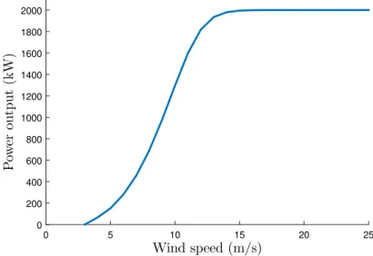
The model of a wind farm production considered in this article is a simplified computation of the output power in kW as a function of the wind speed in m/s. The model is based on the power curve of the chosen wind turbine and is basically a power flow model that considers bulk production losses and potential energy variation with the height of the turbine.
In this article we will focus on a variable speed turbine, rated 2 MW, with a 80 m diameter.
In this model the real output power is computed by a correction of the power curve output power by subtraction of the bulk productions losses:
˜
PW T =(1 − losses) × PW T (1)
where ˜PW T and PW T are the wind farm output power with and without losses and the total losses are estimated at
12.9% representative of wake effect, availability, electrical efficiency, environmental factors losses. These production losses are based on real data provided by our industrial partner, which is a major and experienced player among wind power producers in France.
Fig. 1. Power curve for the 2 MW wind turbine.
A final correction to the output power consists in the potential energy variation with the height of the turbine. It is the impact of the difference height between wind measurements and the actual turbine hub. The wind shear effect may be estimated using the following algorithmic law:
Uhub
Vmeas
= ln(zhub/z0) ln(zmeas/z0)
(2) where U and z are respectively the wind speed and height, subscripts hub and meas denote the turbine hub and the wind measurement and z0 is a height reference corresponding to the terrain roughness index. For a rough pasture
terrain, z0=0.01 m.
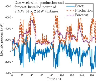
Wind measurements and forecast data used in this article were provided for a site in Guadeloupe island. The wind farm is composed of four 2 MW turbines, for a total installed power of 8 MW. The annual energy output is expected to be around 16 GWh, therefore the load factor is assessed around 23%. The turbine power curve and a one week sample of wind power production and forecast are presented inFigs. 1and2respectively.
A synthetic data generation methodology has been developed to fill for a complete year of wind measurements and forecast. This method can also be used to generate the input vectors needed for the system simulation at the scale of the system life span (several years). We use the phase-randomizing method proposed in [22].
The method is an extension of the multi-variable case of an algorithm based on the Fourier transform to generate data to replace a limited time horizon data set. The new generated data set is not only representative of the correlation between the variables (wind measurement and forecast in this case), but also of the correlation between time steps in the time series. For the mono-variable case, two methods are normally used to tackle this kind of problem. In the first method, a model of the original data set is directly identified, using an ARMA model. In the second, the Fourier transform is applied to the data set, a random variable is introduced to the phases and the inverse transform is computed.
For a time series x(t ), composed of N values taken at a regular time step t = t0, t1, . . . , tN −1=0, ∆t, . . . , (N −
1)∆t , the Fourier transform is obtained by applying the F operator: X( f ) = F {x(t )} =
N −1
∑
n=0
x(tn)e2πi f n∆t (3)
This complex value may be rewritten as:
Fig. 2. One week sample of wind production and forecast.
where A( f ) is the amplitude andφ( f ) is the phase. A phase-randomizing Fourier transform is built by introducing a random rotation Φ to the phaseφ, this is:
˜
X( f ) = A( f )ei[φ( f )+Φ( f )] (5)
Applying the inverse transform the new data set is obtained: ˜
x(t ) = F−1{ ˜X( f )} = F−1{X( f )eiϕ( f )} (6)
By mathematical principle, the time series ˜x(t ) will have the same spectral power density and the same autocorrelation as x(t ).
For the multi-variable case, let us suppose that we have m simultaneously measured variables x1(t ), x2(t ), . . . , xm(t )
with X1(t ), X2(t ), . . . , Xm(t ) their Fourier transform. The inter-correlation between the j th and kth variables is defined
by:
Cj k(τ) = ⟨xj(τ)xk(t −τ)⟩ (7)
The Fourier transform of this inter-correlation gives us the inter-spectrum between variables:
X∗j( f )Xk( f ) = Aj( f ) Ak( f )ei[φk( f )−φj( f )] (8)
Here X∗j( f )Xk( f ) must be fixed for each pair ( j, k), for auto-correlations and inter-correlations to be guaranteed. As
we want to add a phase to the equation, a random sequenceϕ( f ) must be added to φ( f ) for each j. This is: ˜
xj(t ) = F−1{Xj( f )eiϕ( f )} (9)
2.2. Li-Ion battery model
A classic optimization-oriented model to represent the Li-Ion battery is limited to the definition of a charge/ discharge efficiency. A presentation of this type of model is given in detail in [1].
This model has been widely used in optimization-oriented modeling approaches. Despite the simplicity and fast simulation times offered by this type of model, several problems arise with this methodology. A first problem relies on
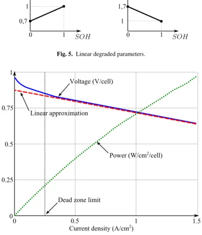
Fig. 5. Linear degraded parameters.
Fig. 6. Linear approximation on the FC polarization curve.
These parameters are directly introduced in Eqs. (10) and(11). Fig. 5 shows an outline of the linear parameter degradation characteristics.
2.3. H2/O2 battery model
The model presented in this section describes the behavior of a H2/O2 battery from an energetic perspective. The H2/O2 energy storage system is composed of an electrolyzer, a fuel cell and H2 and O2 tanks. The model presented in this article is derived from a knowledge model developed in LAPLACE laboratory and partially presented in [7].
For the fuel cell (FC) model, we suppose a linear behavior on the V–I polarization curve, accepting an important modeling error for current densities between 0.05 and 0.25 A/cm2. This linear approximation is graphically described
inFig. 6. However, this assumption is acceptable since a dead band is defined at low current densities for security
reasons (crossover) and to guarantee the auxiliary systems energy consumption (an autonomous FC system is considered). This means that there is a minimum power Pmi naux from which the FC begins delivering effective
power.
The net output power of the FC PoutF C is defined as the power delivered by the FC after deduction of auxiliary systems consumption. The auxiliary systems power consumption is defined by:
Paux =Pmi naux +k Pst ack (20)
where k is the fraction of the power consumed by the auxiliary systems in terms of the nominal FC stack power. The net output power of the FC is given by:
used in applications as in the software HOMER from NREL and in the literature for several techno-economical analysis with renewable energies in [14,4,2,20].
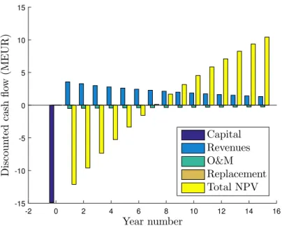
The N P V is a method used to analyze an investment taking account of the costs (negative cash flows) and revenues (positives cash flows) over a complete analysis period. It is defined for a present moment for cash flows obtained over Nyears, this is:
N P V = N ∑ n=0 Fn (1 + dn)n (39) where Fn is the total cash flow for each annuity n, dn is the nominal discount rate and N is the total number of
annuities. The initial investment is accounted as a negative cash flow for year zero (F0 = −Initial investment). For
each annuity from n = 1, . . . , N we compute the following coefficients:
C O E F Fe=(1 + e)n (40)
P V I Fn =
1 (1 + dn)n
(41) where e is the mean annual inflation rate. The present value of the replacement cost of a storage equipment is obtained using:
P V r eplcostSt o=
r eplcostSt o×i nvtSt o
(1 + dn)r
(42) where r is the year of replacement. Then the equipment depreciation Dn is estimated using the mixed depreciation
law proposed in [27]. With Dna new value of the equipment net book value is estimated for annuity n using:
net Book V aln =net Book V aln−1−Dn (43)
The annual revenues Revnadjusted for the period inflation rate may be computed using the energy effectively injected
to the grid Egr i d(in MWh) and the feed-in-tariff F I T (in EUR/MWh):
Revn=Egr i d×F I T × C O E F Fe (44)
Then the net taxable income net T ax I nn, the tax on total income I nT axn and the resulting after tax cash
a f t er T axCashnare obtained with:
net T ax I nn =Revn− · · ·
. . . − O Mcostt ot×C O E F Fe−Dn (45)
I nT axn =T ax Rat e × net T ax I nn (46)
a f t er T axCashn =Revn− · · ·
. . . − O Mcostt ot×C O E F Fe− f ed I nT axn (47)
Finally, the N P V for each annuity N P Vn, its cumulated value and the global N P V for the total analysis period are
computed using:
N P Vn =a f t er T axCashn×P V I Fn (48)
N P V cumuln =N P V cumuln−1+N P Vn (49)
N P V = N P V cumuln−i nvtt ot (50)
The LC O E is finally obtained with an iterative method for varying values of FIT. The LC O E is obtained for the FIT value that yields the ratio N P V/invtt ot =0 at the end of the analysis period.
3. Energy management strategy 3.1. Ancillary services
Many different power delivery services may be defined for this type of power producer in island grids. In this work, we will focus on two main “ancillary services”:
• Day-ahead commitment with power production smoothing: a power commitment is defined as a discrete 30-min constant power profile that is generally obtained from a production forecast profile. This commitment should be respected inside a tolerance layer of 25% of the nominal installed power for the first year of operation, 20% for the second year and 15% from the third year and to the end of the delivery agreement.
• Primary energy reserve: a second service considered is a power reserve of 10% the nominal installed power that may be demanded one time per day during 15 min. This active power reserve is designed by the utility operator to achieve efficient control of the power grid area frequency.
The energy management block is presented in the following section but it may be composed of any desired management strategy from heuristic rule-based to optimal control strategies. The simulation is a power balance of the power produced by the RES and the power charged/discharged by the storage devices at the plant power delivery point and for each time step ∆t . The inputs of the energy management block are the power production Ppr od and
commitment Pengfor the present time step k and the system states (notably the storage S OC) for the previous time step
k −1. The outputs are the power reference for storage devices PR E F
st o and a power reference for production degradation
PR E F
pr od for the special cases with excess produced energy that cannot be charged by the storage devices (production
with MPPT degradation). These power references are directly the inputs for the physical system simulation block. After the simulation of the power balance at the delivery bus, the output of this second block is the power injected to the grid Pgr i d, the wasted power due to MPPT degradation Pwasted and the power not-supplied during a violation of
the day-ahead commitment Pnot suppli ed.
The violation of the day-ahead commitment is defined as a “commitment failure” (C F ) and is computed using: C F(%) = 100% × 1 N N ∑ k=1 C F(k) (51)
where C F (k) is a counter of a lower bound violation of the tolerance layer at each time step. This definition is quite similar to the variable Loss of Power Supply Probability (LPSP) thoroughly found in the literature. During a C F , the day-ahead commitment is not respected as a consequence of a low production output, an insufficient stored energy or a technical failure. A high bound violation of the tolerance layer is not considered as a system failure as it can be corrected with a MPPT degradation. A C F is accounted during a lower bound violation of the tolerance layer (for 1 min average power metering) and for a period of 10 min after the grid injected power is again inside the tolerance layer. The power delivered during a C F is not paid by the utility operator.
3.2. Heuristic energy management
The energy management strategy presented in this article is a basic rule-based algorithm designed with a certain trade-off margin between a good tracking of the day-ahead commitment and an efficient use of the storage device for an enhanced lifespan. The strategy is based on the position of the actual power production Ppr od as a function of the
tolerance layer. The energy management problem is then divided into three regions:
• If Ppr od > Peng+t ol: this is a situation where an excess of produced energy may occur. In this case we define a
desired power level to be delivered to the grid, we call this the goal power Pgoalfixed in this case at upper bound
of the tolerance layer Pgoal = Peng+t ol. The storage power reference is defined as: Pst oR E F = Pgoal−Ppr od.
If the battery is no longer able to absorb this excess power (reaching the maximum battery S OC or nominal power limitation) then the producer MPPT is degraded.
• If Ppr od < Peng−t ol: this is a situation where a lack of produced energy may occur. In this case the desired
goal power is fixed at the lower bound of the tolerance layer Pgoal =Peng−t ol. The storage power reference is
defined as: PR E F
st o =Pgoal−Ppr od. If the battery is no longer able to provide the needed power then a C F (k) = 1
is accounted.
• If Peng−t ol ≤ Ppr od≤ Peng+t ol: the power production is inside the tolerance layer. The storage is used only if
Peng−Ppr od< 0 and SOC < threshold (with the threshold defined in this case at 60%). If the condition holds,
then the power reference for the storage is PR E F
st o =Pgoal−Ppr odwith Pgoal =Peng. Otherwise Pst oR E F =0 and
Fig. 14. Simulation results WT+Li-Ion: cash flow and N PC progress.
Fig. 15. Simulation results WT+Li-Ion: system costs by component.
results and the plant costs obtained are promising in the insular context and in comparison with other traditional power plant technologies. The modeling tool includes ageing models of the storage devices. This modeling tool is suitable for decision making in planning stages. Complete sensitivity studies may be conducted with this type of tool, with some examples presented in this article. The modeling tool has been completed with other RES sources such as PV. The obtained results show a clear advantage for a hybrid system with only Li-Ion batteries, despite a promising future for the complete hybrid option including H2/O2 storage. Other future works may involve a complete sensitivity study of varying parameters and towards the implementation of an optimized energy management strategy.
[18] N.A. Luu, Q.T. Tran, S. Bacha, V.L. Nguyen, Optimal sizing of a grid-connected microgrid, in: 2015 IEEE Inter. Conf. on Ind. Tech., ICIT, pp. 2869–2874.
[19] E. Nasrolahpour, S.J. Kazempour, H. Zareipour, W.D. Rosehart, Strategic sizing of energy storage facilities in electricity markets, IEEE Trans. Sust. Energy 7 (4) (2016) 1462–1472.
[20] M. O’Connor, T. Lewis, G. Dalton, Techno-economic performance of the pelamis P1 and wavestar at different ratings and various locations in Europe, Renew. Energy 50 (2013) 889–900.
[21] P. Pinson, G. Papaefthymiou, B. Klockl, J. Verboomen, Dynamic sizing of energy storage for hedging wind power forecast uncertainty, in: Proceedings of the IEEE PES General Meeting 2009.
[22] D. Prichard, J. Theiler, Generating surrogate data for time series with several simultaneously measured variables, Phys. Rev. Lett. 73 (17) (1994) 951–954.
[23] Y. Riffonneau, S. Bacha, F. Barruel, S. Ploix, Opt. PF management for grid connected PV systems with batteries, IEEE Trans. Sust. Energy 2 (3) (2011) 309–320.
[24] R. Rigo-Mariani, B. Sareni, X. Roboam, A fast optimization strategy for power dispatching in a microgrid with storage, in: IECON 2013, pp. 7902–7907.
[25] Y. Ru, J. Kleissl, S. Martinez, Storage size determination for grid-connected photovoltaic systems, IEEE Trans. Sust. Energy 4 (1) (2013) 68–81.
[26] SAFT, Lithium-Ion Battery Life: Solar Photovoltaics (PV) - Energy Storage Systems (ESS), Technical Report Document No. 21893-20514, SAFT, 2014.
[27] W. Short, D.J. Packey, T. Holt, A Manual for the Economic Evaluation of Energy Efficiency and Renewable Energy Technologies, Technical Report NREL/TP-462-5173, National Renewable Energy Laboratory, 1995.