1 This is an accepted manuscript of an article published Cybergeo Geography on June 4 2015, available at http://dx.doi.org/10.4000/cybergeo.27035
Please cite as:
Apparicio, Philippe, Mylène Riva, and Anne-Marie Séguin. 2015. "A comparison of two methods for classifying trajectories: a case study on neighbourhood poverty at the intrametropolitan level in Montreal." Cybergeo : European Journal of Geography (727). doi: 10.4000/cybergeo.27035.
2 A comparison of two methods for classifying trajectories: a case study on neighbourhood poverty at the intra-metropolitan level in Montreal
Philippe Apparicio, Mylène Riva, Anne-Marie Séguin Philippe Apparicio
Professor
INRS Urbanisation Culture Société
385 rue Sherbrooke Est, Montréal (QC), Canada, H2X 1E3 Philippe_apparicio@ucs.inrs.ca
Mylène Riva Assistant Professor
Department of Social and Preventive Medicine, Population Health and Optimal Practices in Health Research Unit, CHU de Québec Research Centre, Université Laval
Mylene.Riva@crchudequebec.ulaval.ca Anne-Marie Séguin
Professor
INRS Urbanisation Culture Société
385 rue Sherbrooke Est, Montréal (QC), Canada, H2X 1E3 anne-marie_seguin@ucs.inrs.ca
In recent years several studies have examined changes in the distribution of poverty in the North American cities, with most empirical work assessing neighbourhood change between two time points. This paper aims to make a methodological contribution to the study of neighbourhood change, by comparing two classification methods, one classical (k-means clustering) the other more novel (Latent Class Growth Modelling; LCGM) to identify groups of census tracts having followed similar trajectories of poverty in the Montreal metropolitan area, Canada. Here trajectories of poverty are measured over a twenty year period, using five time points. The relative performance of the LCGM vs. the k-means clustering was assessed using a series of multinomial logistic regressions examining how different socioeconomic variables were associated with the trajectories of poverty. Results showed that k-means and LCGM identified similar groups of census tracts characterised by ascending, descending, or stable poverty levels throughout the period, with LGCM only marginally outperforming k-means clustering.
Latent class growth modelling; k-means; clustering; Neighborhood change; poverty; trajectories, Montreal
3 Durant les dernières années, plusieurs auteurs ont examiné les changements dans la répartition de la pauvreté au sein des villes nord-américaines. La plupart de ces travaux empiriques ont porté sur deux points dans le temps. Cet article vise à apporter une contribution méthodologique pour l'étude du changement dans les quartiers, en comparant deux méthodes de classification : l’une bien connue (le K-means) et l’autre plus récente (Latent Class Growth Modelling; LCGM) pour identifier les groupes de secteurs de recensement ayant suivi des trajectoires de pauvreté similaires dans la région métropolitaine de Montréal (Canada). Les trajectoires sont identifiées sur une période de vingt ans en utilisant cinq années de recensement (1986, 1991, 1996, 2001, 2006). La performance relative du LCGM versus le k-means a été évaluée à l'aide d'une série de régressions logistiques multinomiales examinant comment les différentes variables socio-économiques ont été associées avec les trajectoires de pauvreté. Les deux méthodes permettent d’identifier à la fois des trajectoires de pauvreté stables, ascendantes et descendantes. Toutefois, le LCGM est très légèrement plus performant que le k-means.
Modélisation de variable latente de croissance; k-means; classification; pauvreté; trajectoires; Montréal
Introduction
In the past decades, rapid urban expansion in conjunction with a growing income gap (Heisz et al., 2006) and structural forces such as economic restructuring, demographic shifts, as well as changes in government policies have impacted on the socioeconomic divisions in North American cities (Kitchen et al., 2009; Walks, 2001), as well in European cities (Van Kempen et al., 2009). Hence the spatial dimension of urban and neighbourhood change in cities of developed countries is receiving increasing attention (Kitchen et al., 2009). To date, most of the empirical work has examined neighbourhood change between two time points (see for example the recent works of Mikelbank, 2006; Reibel et al., 2011; Vicino, 2008). Except the recent work of Mikelbank (2011) on the Cleveland-Akron metropolitan area, and the one of Apparicio et al. (2012) on Montreal, few studies have identified trajectories of change in socioeconomic conditions, allowing the direction and magnitude of trends to vary between more than two time points, and how this change plays out at the intra-metropolitan level. Yet processes of gentrification (Berry, 1986; Bunting et al., 1988; Clark, 1987; Ley, 1986) and the impoverishment of inner suburbs documented in more recent work (Cooke et al., 2006; Jargowsky, 2003; Lee et al., 2007; McConville et al., 2003; Short et al., 2007) are indicative of important transformations in the urban social geography, and are important to grasp in their dimensions.
In a recent paper (Apparicio et al., 2012), we use a new clustering technique for longitudinal data – latent class growth model (LCGM) – to identify trajectories of neighbourhood poverty in Montreal over five consecutive census years (1986 to 2006). Then, we conduct a multinomial logistic regression analysis for modelling the trajectories obtained by the LCGM.
Although based on the same spatial dataset of that previous study, our objective in this paper is quite different. While the classification methods such as k-means clustering and hierarchical cluster analysis are largely used in quantitative geography, the LCGM approach is still little-known by many geographers. Consequently, the purpose of this study is to compare LCGM versus the k-means clustering to assess which method performs better in identifying trajectories of neighbourhood change. The potential benefits of the LCGM in quantitative research in urban
4 geography are discussed as well. Indeed, this approach for classifying spatial longitudinal data can be applied to analyze the neighbourhood changes such as poverty, immigration, ethnic or social diversity, unemployment, etc.
For illustrative purposes, we analyze the geography of low-income population as measured at five time points over a 20-year period in Montreal, i.e. the trajectories of relative poverty at the neighbourhood level. In practical terms, the paper aims to identify groups of neighbourhoods characterized by a similar pattern of change in their poverty levels. The present study therefore attempts primarily to make a methodological contribution to the study of neighbourhood change.
Background
Studying neighbourhood poverty change
Several studies concerned with changes in high-poverty neighbourhood, at least in the USA, have focussed on the growth of these neighbourhoods in suburban areas, and especially in inner-ring suburbs. Some studies aim to identify the evolution in the distribution of poverty zones in metropolitan areas, notably by opposing the central city to inner-ring suburbs (Cooke et al., 2006; Lee, 2011; Lee et al., 2007). Other research, such as the study by McConville and Ong (2003), is interested by the trajectories of poor neighbourhood, i.e. whether they stayed poor, worsen or improved over time, in relation to change in other neighbourhood conditions, e.g. ethnic, immigration, education, employment and family profiles.
In Canada, few studies have examined transformations of poverty neighbourhood. In 2000, Ley and Smith (2000) noted the changing nature of some census tracts in Toronto, Montreal and Vancouver over a twenty year period, observing that deprived neighbourhoods in 1971 were not necessarily deprived by 1991 and inversely, none-deprived neighbourhood in 1971 could have become deprived by 1991. Their observations were based on several cumulative indicators associated with deprivation (measured using thresholds) measured first in 1971 and then in 1991. Using census data, Heisz and McLeod (2006) showed that both the proportion of low-income neighbourhoods and their spatial distribution across the different Canadian metropolitan areas varied between 1981 and 2001. For example, they observed that, compared to 1981, low-income neighbourhoods in Montreal and Toronto were less likely to be located in inner city neighbourhoods by 2001 and more in inner-ring suburban areas. Although this study by Heisz and McLeod identified broad trends for each metropolitan area, the authors did not identify neighbourhood trajectories per se.
A study by Kitchen and Williams (2009) set in Saskatoon, a Canadian metropolitan area of moderate size, analyzed neighbourhood change between 1991 and 2001, considering two ‘sub-periods’, 1991-1996 and 1996-2001. Their analyses considered the socioeconomic profile of 58 neighbourhoods at the beginning of the period (1991), classifying them as low, middle or high socioeconomic status (SES) neighbourhoods. Neighbourhoods were then characterised as following three possible trajectories of change in SES between 1991 and 2001, i.e. decline, improvement or stability. Kitchen and Williams study (2009) is interesting as it considered socioeconomic conditions at the beginning of the study period and their change over a 10 year period. Yet ten years of observation might be too short to identify important changes in urban processes such as filtering down (out-migration of households to newer and more elaborate dwellings and in-migration of households of lesser wealth and lower social status), gentrification, and the suburbanization of poverty.
5 Our study proposes to analyse trajectories of neighbourhood poverty on a longer 20-year period. As Kitchen and Williams (2009), we consider poverty levels at the beginning of the period, i.e. 1986, but also neighbourhood poverty levels in 1991, 1996, 2001 and 2006. Thus, over time, a neighbourhood could be characterised by an ascending trajectory, then a descending trajectory, followed by a stable level of poverty, to a declining slope at the end of the study period. At each time point poverty is measured as a continuous variable. This will allow us to identify trajectories with more precision and to identify an optimal number of trajectories. Statistically, this will be achieved by applying and comparing two clustering techniques to group neighbourhoods having followed similar trajectories of change in poverty levels. Hence the objective of this paper is essentially a methodological one, i.e. to identify a clustering method most suited to measure neighbourhood change. We will see later that these approaches allow maximising variation between trajectories and minimising variation within trajectories. This step is crucial if the aim is to identify the determinants of neighbourhood change and to measure their relative importance. This paper builds on previous work by defining trajectories of poverty using five time points, allowing for the magnitude and direction change in poverty to vary at each time point.
This precision, however, comes with methodological challenges, including the construction of a longitudinal database at the intra-metropolitan scale (i.e. at the census tract level) with comparable and harmonised socioeconomic data and geographical boundaries across several census years. Another methodological challenge is to find the most accurate approach to group neighbourhoods characterized by a similar evolution of their poor population over time, with each group (i.e. trajectory) being most different amongst themselves. In the next section, we discuss two possible techniques.
Identifying trajectories of neighbourhood change at the
intra-metropolitan level: the possibilities provided by k-means clustering and
latent class growth modelling
Modelling social change has mainly been tackled from time-series and econometric perspectives, namely to study economic cycles and changes in labour markets at broad geographic levels. It is also possible to envision trajectories of change in terms of ‘clusters’ of areas having followed a similar pattern of change along a variable (or variables) of interest over time. To date unsupervised clustering techniques such as hierarchical cluster analysis (HCA) and k-means clustering, or extensions of k-means (eg. fuzzy k-means (Friedman et al., 1998), partitioning around the medoid (Kaufman et al., 2005); see Jain (2007) for a description and a comparison of several extensions of the k-means clustering), mainstreamed in urban geography and social sciences, have mainly been applied to cluster spatial ‘objects’ with similar characteristics at one point in time (see for example Mikelbank, 2004; Vicino et al., 2011) and less often at two points in times (Reibel et al., 2007, 2011; Vicino, 2008).
However, it is possible to apply these ‘classical’ clustering techniques to a longitudinal dataset to identify neighbourhood trajectories. For example, Mikelbank (2011) applied an HCA to group census tracts along several demographic, housing and socioeconomic variables extracted from four censuses (1970, 1980, 1990, 2000). These variables were standardized (z-scores) at each time point, and were then appended in one table, on which an HCA was computed. This allowed identifying five types of neighbourhoods over the period: struggling, struggling African American, stability, new starts, and suburbia. Thus, a census tract could belong to the same neighborhood type during the four census years, or it could change type one
6 or more times. Finally, Mikelbank (2011) built several transition tables to identify stability or change in neighbourhood trajectories across two years or all the time periods.
Whereas it is possible to apply classical clustering techniques to longitudinal spatial datasets, new semi-parametric analytical procedures have recently been developed to groups ‘objects’ having followed similar trends over time, namely Latent Class Growth Models (LCGM) (Nagin, 2005). To date, LCGM has mainly been applied in psychology (Nagin, 2005) and epidemiology, for example, to group individuals with similar trajectories of change in health-related behaviours (Barnett et al., 2008; Brookmeyer et al., 2009). To our knowledge, it has been applied to spatial data to examine trajectories of change within a metropolitan area or a country in only three studies (Apparicio et al., 2012; Pearson et al., 2013; Riva et al., 2012).
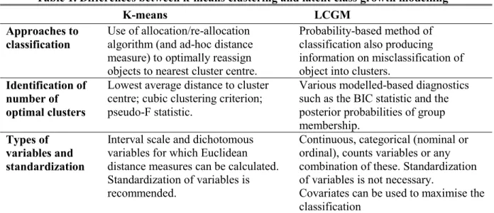
K-means and LCGM are statistical clustering techniques that can be applied to classify objects (i.e. census tracts) into k number of clusters (i.e. trajectories) with similar change in a variable (i.e. poverty) over time. K-means is an exploratory statistical clustering technique that uses an allocation/re-allocation algorithm to optimally reassign census tracts to the nearest cluster centroid (Everitt et al., 2001). The goal is to maximize between clusters variations and to minimize within cluster variations, and thus to group into k types of local areas having followed similar trajectories of change in poverty over the study period. Some statistical software, e.g. SAS, optimizes the choice of initial cluster centres; thus, the random selection of cluster centres, potentially leading to different solution when the model is re-run, is no longer being a ‘problem’. Compared to HCA algorithms, the number of k must be chosen a priori in k-means clustering and there are several methods to identify the optimal cluster solution (Milligan et al., 1985) including, amongst others: the Pseudo-F statistic (Calińskia et al., 2007); the Cubic Clustering Criterion (Sarle, 1983); or a more discursive method (Tibshirani et al., 2001) consisting of plotting the average distance to cluster centroid for each cluster solution and visually identifying the optimal cluster solution where there is a natural levelling off in the distribution (the ‘elbow criterion’).
LCGM is a semi‐parametric approach to classification (Andruff et al., 2009; Collins et al., 2009; Duncan et al., 2009). Although each census tract will follow a unique trajectory of changing poverty levels, the heterogeneity in the distribution of census tracts is summarized by a finite set of polynomial functions, each corresponding to a discrete class or trajectory (Andruff et al., 2009; Nagin, 2005). Because the magnitude and direction of change can freely vary between trajectories, a set of model parameters, i.e. intercept and slopes, is estimated for each trajectory (Andruff et al., 2009; Nagin, 2005). For each trajectory, the slope and intercept are treated as fixed (equal) between census tracts. In LCGM, the optimal number of classes is informed by a built-up modelling approach whereby the modelling starts with a one-class model, and classes are subsequently added to evaluate improvement in model fit. The model providing the best fit to the data is identified by interpreting and comparing several diagnostic tools, including the model with the lowest Bayesian Information Criterion (BIC) and posterior probabilities of group membership (a maximum‐probability assignment rule is used to assign each individual to the trajectory to which it holds the highest posterior membership probability) (Andruff et al., 2009). LCGM is now relatively easy to apply in software such as SAS (ProcTRAJ) (Jones et al., 2007), Mplus (Muthén & Muthén), and LatentGOLD (Statistical Innovations). The main differences between k-means and LCGM are summarised in Table 1 (adapted from LatentGold website:
http://www.statisticalinnovations.com/articles/kmeans2a.htm).
The underlying principles of k-means and LCGM are thus different: one is a descriptive/ exploratory technique whereas the other adopts a semi-parametric approach to classification. It is
7 also worth noting that K-Means requires continuous or dichotomous variables while LCGM can be applied to any type of distribution (continuous, ordinal, nominal, count and binomial). In this study, the variable used for the classification –i.e. the location quotient– is continuous. Yet no studies have compared how the methods fare in generating groups of spatial units having followed similar trajectories of change.
Table 1. Differences between k-means clustering and latent class growth modelling
K-means LCGM
Approaches to classification
Use of allocation/re-allocation algorithm (and ad-hoc distance measure) to optimally reassign objects to nearest cluster centre.
Probability-based method of classification also producing information on misclassification of object into clusters.
Identification of number of optimal clusters
Lowest average distance to cluster centre; cubic clustering criterion; pseudo-F statistic.
Various modelled-based diagnostics such as the BIC statistic and the posterior probabilities of group membership.
Types of variables and standardization
Interval scale and dichotomous variables for which Euclidean distance measures can be calculated. Standardization of variables is recommended.
Continuous, categorical (nominal or ordinal), counts variables or any combination of these. Standardization of variables is not necessary.
Covariates can be used to maximise the classification
Objectives of the study
Aiming to better characterize trajectories of neighbourhood poverty change, the purpose of this study is to apply and compare two clustering techniques to 20 years of census data (five time points) to identify groups of neighbourhoods having followed similar trajectory of poverty between 1986 and 2006. Weapply both k-means and LCGM techniques to assess which method performs better in identifying trajectories of poverty. The selection of the most accurate classification represents a crucial step before developing explanatory models of socioeconomic changes operating in metropolitan areas.
Several studies have demonstrated that the clustering accuracy of the k-means is superior to that of HCA, especially when computed on large data sets (see for example Abbas, 2008). In addition, results of HCA vary according to the distance metric (Euclidian distance, squared Euclidean distance, Mahalanobis distance, etc.) and the cluster method (single, complete, median, centroid linkages, Ward’s method, etc.). To prevent comparing results of LCGM models to several variants of the HCA, we opted for k-means clustering.
Material and methods
Study area and data
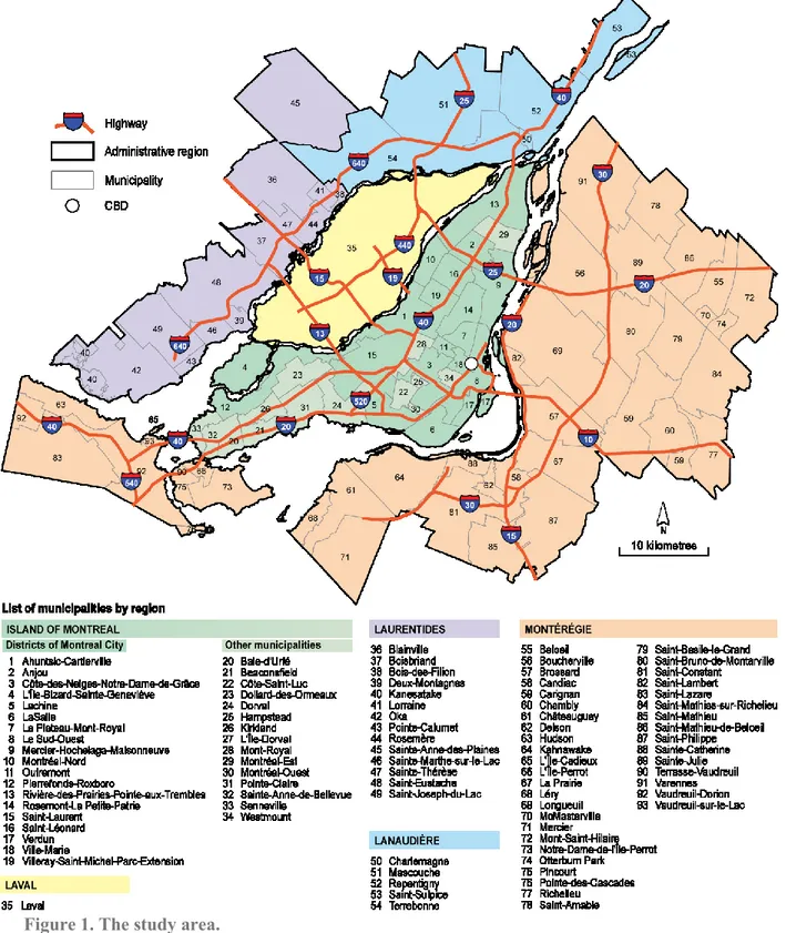
This study is set in Canada, in the Montreal Census Metropolitan Area (CMA) comprising a population of about 3.64 million inhabitants spread over a territory of 4,259 km2 in 2006
(Statistics Canada, 2007). Intra-metropolitan areas are defined using census tract boundaries. Administrative and census geographical boundaries in the Montreal CMA have changed considerably between 1986 and 2006: the number of census tracts increased from 698 to 825 over this period. Harmonisation of the geographic boundaries of census tracts was therefore
8 necessary. Starting with the 1986 census tracts geographic boundaries (the earliest time point), this was achieved by aggregating contiguous census tracts in order to obtain comparable boundaries across all census years. A total of 611 census tracts was obtained.
9 Relative poverty was measured every five years between 1986 and 2006 using data from the Canadian Census using the ‘low-income cut-offs’ variable calculated by Statistics Canada. This variable corresponds to the income level at which a household spend 20% or more of its income (before tax) on the basics (i.e. food, shelter and clothing) than does the average household of similar size (Statistics Canada, 2011).
This measure is the only one in the Canadian census that allows identifying low-income persons or families at a small geographical scale, e.g. census tracts (Apparicio et al., 2007; Séguin et al., 2012). Because comparing ‘crude’ poverty levels rates between census tracts and across time might be influenced by the changing economy (i.e. periods of recession or economic prosperity), poverty was modelled as a ‘location quotient’ so that, at each time point, the poverty rate of each census tract was divided by the rate observed for CMA as a whole; we are thus using a measure of relative poverty concentration. The proportion of low-income population in the CMA at each time point is showed in Table 2. The location quotient gives an overview of how, at any time, local poverty levels compare to the CMA average. This measure of concentration is largely used in urban and regional studies (Mikelbank, 2006; Shearmur et al., 2008; Shearmur et al., 2009; Vicino et al., 2011; Walks et al., 2008), and is computed as follow:
Where:
xi= low income population in private households the census tract i;
ti= total persons in private households in the census tract i;
X= low income population in private households in the CMA; T= total persons in private households in the CMA.
A location quotient greater than 1 indicates a concentration of poverty (i.e. a percentage of low-income population higher than that of the CMA) whereas a value below 1 indicates an underrepresentation of poverty (i.e. a percentage of low-income population lower than that of the CMA).
Table 2. Description of indicators of poverty for the Montreal CMA between 1986 and 2006a
Census year 1986 1991 1996 2001 2006
Total population 2,826,270 3,019,350 3,125,545 3,208,860 3,363,975 Low-income population 609,175 666,680 863,745 723,670 728,220
% 21.55 22.08 27.64 22.55 21.65
Unemployment rate 11.32 11.69 11.22 7.52 7.01
Lone parent families (%) 15.92 15.73 17.55 18.23 18.24
One-person households (%) 25.31 27.34 29.55 31.19 31.99
People aged ≥ 65 years (%) 9.26 10.26 11.09 11.97 12.70
Recent immigrants (%) 1.27 2.73 4.21 3.46 4.77
Low education population (%)b 39.76 34.96 31.51 25.87 21.61
University education (%)c 20.74 13.42 26.05 26.27 25.14
Renters (%) 55.54 53.65 52.19 50.45 47.51
a All variables are calculated for the CMA boundaries of 1986.
b For 1986, 1991 and 1996 censuses: Population 15 years and over with less than grade 13 without
secondary school certificate; For 2001 census: Population 20 years and over with less than grade 13 without secondary school certificate; For 2006 census, population 15 years and over without diploma.
c Population 15 years and over, except for the 2001 census where this information is available for
population aged 20 years and over.
) / /( ) / (x t X T LQi i i
10
LCGM and k-means clustering methods to identify trajectories of
relative poverty
Generation of trajectories of neighbourhood poverty was first conducted using LCGM, as this technique provides diagnostic statistics regarding the optimal cluster solution. We set as an initial criterion that each cluster/trajectory needed a minimum of 5% of the 611 census tracts, so a minimum of 30 census tracts per trajectory. This was set to ensure a minimum of observations per trajectory in later validation stage (e.g. and in line with minimum requirement of observation for regression analysis). As we had no a priori for the optimal number of classes, LCGM was conducted for 5 to 20 classes; a minimum of 5 classes was set in order to have a minimum of differentiation between groups of census tracts. The optimal cluster solution is identified by: 1) a minimum of 5% of census tracts per trajectories; and 2) the lowest BIC value. Analyses were conducted in LatentGOLD software (Statistical Innovations).
K-means clustering was conducted in SAS 9.2 (SAS Institute Inc), specifying again 5 to 20 clusters. The value of the average distance to cluster centroid for each cluster solution was plotted to identify a ‘natural break’ in the distribution, indicating the optimal cluster solution. In the end, the choice of the optimal number of cluster solutions was informed by the LCGM solution providing the best fit to the data.
Statistical analyses
To assess the relative performance of the LCGM vs. the k-means clustering in identifying trajectories of relative poverty, two sets of analyses were conducted. First, in a multinomial logistic regression (MLR), the variables used for the classification (i.e. the location quotients from 1986 to 2006) were modelled as predictors of the trajectories (trajectories are modelled as a categorical dependent variable). This approach is some form of discriminant analysis, used to test the performance of different methods of classification (see for example Magidson et al., 2002) or different numbers of cluster solutions. The idea here is to use the R-Square and model fit statistics from this analysis to inform which of the k-means and LCGM cluster solutions better summarizes the variation in poverty concentration.
A second series of MLR was then conducted to empirically examine how a set of predictors theoretically associated with poverty explain each trajectory: unemployment rate, single parent families (%), one-person households (%), the elderly (≥ 65 years) (%), recent immigrants (%), low education population (%), university education (%) and renters (%) (see Table 2 for a description of the values taken by the predictors between 1986 and 2006 for the study region). These variables were retained because recent studies have demonstrated that they are strongly associated with the spatial distribution of poverty across the Montreal CMA at the census tract level (Apparicio et al., 2007; Séguin et al., 2012). In separate MLR models, these predictors were modelled at the start of the period, i.e. 1986, at end, i.e. in 2006, and as variation between 1986 and 2006 (e.g. unemployment rate 2006 - unemployment rate 1986). A final model including baseline predictors and variation between 1986 and 2006 was run. For each model, the focus is on the strength (R-Square) and the fit (Akaike Information Criterion [AIC] and Bayesian Information Criterion [BIC]; lowest value of the AIC and BIC are indicative of better model fit) of the model.
11
Results
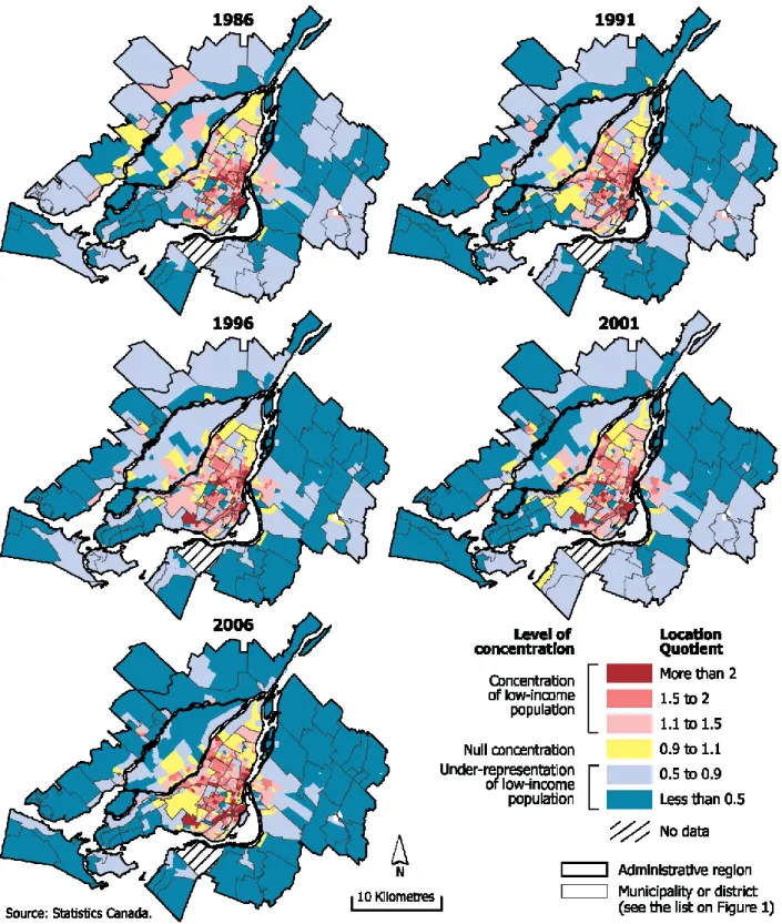
Location quotients of the low-income population for the five census years at the census tract level (CT) are mapped in Figure 2. As reported in previous studies (Apparicio et al., 2007; Séguin et al., 2012), CTs displaying a concentration of poverty are mainly located in the central part of the Island of Montreal, corresponding to inner-city neighbourhoods, whereas CTs characterized by an under-representation of poverty are observed in Laval and the North and South shores, corresponding to suburban areas. Over the 1986-2006 period, the presence of poverty in many central CTs (inner-city neighbourhoods) became less pronounced, while poverty gained grounds outside the central CTs on the island of Montreal in areas urbanized during the 1950’s and 1960’s. Some areas of concentrated poverty located in the northern periphery of the CMA disappeared over the period under study (these are old village centres in municipalities that have witnessed the arrival of new, wealthier populations).
12
Figure 2. Location quotients of relative poverty in Montreal CMA at census tract level (1986-2006).
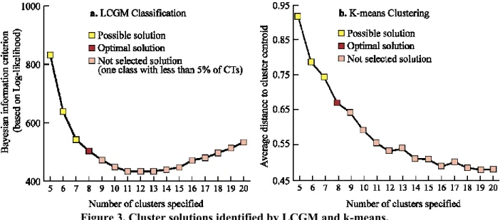
Optimal cluster solution for both the LCGM and k-means clustering are presented in Figure 3. According to the LCGM analysis, the 611 census tracts were optimally classified in eight trajectories, identified by the ‘cluster solution’ insuring a minimum of 5% census tracts per trajectory and with the lowest BIC values. The eight-cluster solution also appeared to fit the data
13 well in the k-means analysis. However, this cluster solution lead to one group of areas comprising less than 5% of census tracts (n=26, 4.3%). Nonetheless, as we elected to use the LCGM model with the best fit to inform the selection of the optimal number of clusters, analyses are conducted on the eight-cluster solution for both the LCGM and k-means.
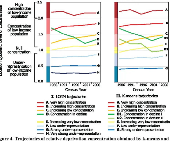
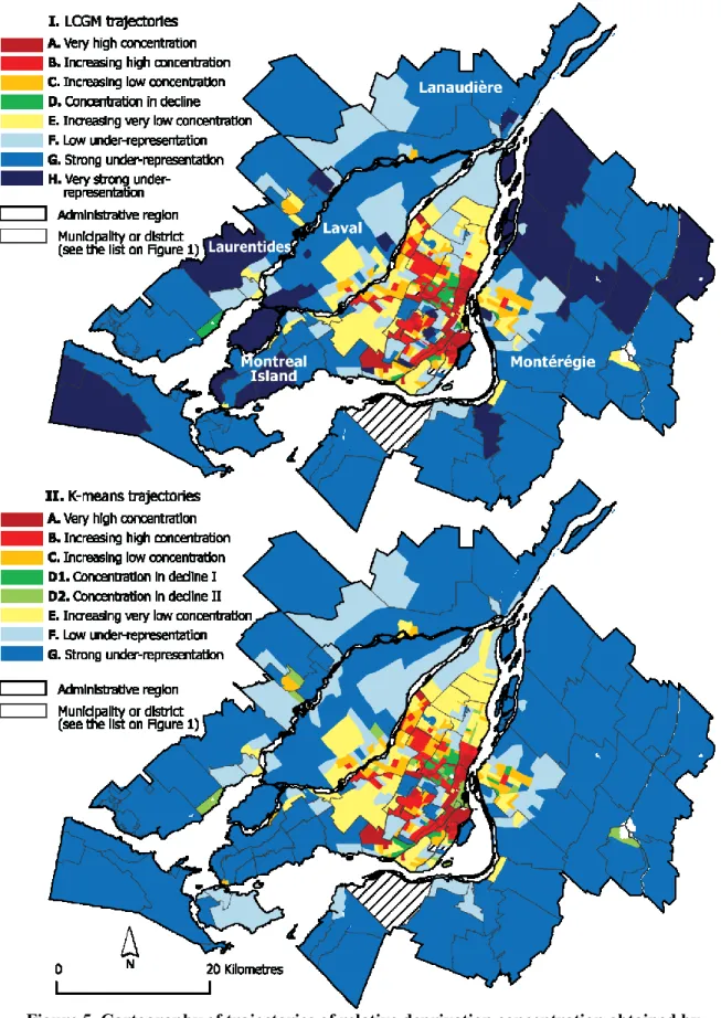
In order to facilitate their analysis, trajectories obtained from the k-means and LCGM were plotted using the ‘gravity centres’ of classes i.e. the mean values of the location quotients for the different classes (Figure 3); the graph easily characterizes each trajectory. In addition, the cartography of census tracts according to their poverty trajectory is shown in the Figure 4. As shown in Figure 4, both methods of classification have allowed to identify groups of census tracts having followed trajectories of increasing or decreasing levels of poverty. This indicates changes in concentration of low-income population in some neighbourhoods in the Montreal CMA. However, for a majority of census tracts, relative poverty levels did not change considerably over the period, as indicated by groups of census tracts with relatively “stable” trajectories throughout the period.
14
Figure 4. Trajectories of relative deprivation concentration obtained by k-means and LCGM methods.
15
Figure 5. Cartography of trajectories of relative deprivation concentration obtained by k-means and LCGM methods.
16 Table 3 illustrates how the 611 census tracts were cross-classified in different trajectories, as per the k-means and LCGM cluster solutions; a rapid inspection of the Table 3 and of the Figure 5 shows that both methods produced relatively similar cluster solutions. The upward trend in poverty concentration in trajectory B is steeper in the LCGM output than in the k-means. Whereas there appears to be two trajectories of decreasing poverty concentration in k-means (D1 and D2), these appeared to be ‘summed’ under one trajectory in LCGM (trajectory D). In addition, LCGM further differentiate between groups of low poverty concentration. Although the LCGM and k-means cluster solutions do not exactly replicate each other, there are some similarities between the results of the two approaches of classification. For example, all observations in LCGM trajectory D are distributed across k-means trajectories D1 (82.2%) and D2 (17.8%). Likewise, all observations in k-means trajectory G are distributed among trajectories G (70.4%) and H (29.6%) of LCGM.
Table 3. Cross-classification of census tracts in the k-means and LCGM cluster solutions
N % (row) LCGM trajectories % (col.) A B C D E F G H Total K -m eans tr aj ect or ies A 65 0 0 0 0 0 0 0 65 100.0 0.0 0.0 0.0 0.0 0.0 0.0 0.0 10.64 80.3 0.0 0.0 0.0 0.0 0.0 0.0 0.0 B 16 66 0 0 0 0 0 0 82 19.5 80.5 0.0 0.0 0.0 0.0 0.0 0.0 13.42 19.8 91.7 0.0 0.0 0.0 0.0 0.0 0.0 C 0 3 60 0 12 0 0 0 75 0.0 4.0 80.0 0.0 16.0 0.0 0.0 0.0 12.27 0.0 4.2 87.0 0.0 12.2 0.0 0.0 0.0 D1 0 3 7 37 0 0 0 0 47 0.0 6.4 14.9 78.7 0.0 0.0 0.0 0.0 7.7 0.0 4.2 10.1 82.2 0.0 0.0 0.0 0.0 D2 0 0 2 8 14 2 0 0 26 0.0 0.0 7.7 30.8 53.9 7.7 0.0 0.0 4.3 0.0 0.0 2.9 17.8 14.3 2.0 0.0 0.0 E 0 0 0 0 72 13 0 0 85 0.0 0.0 0.0 0.0 84.7 15.3 0.0 0.0 13.91 0.0 0.0 0.0 0.0 73.5 13.0 0.0 0.0 F 0 0 0 0 0 85 11 0 96 0.0 0.0 0.0 0.0 0.0 88.5 11.5 0.0 15.7 0.0 0.0 0.0 0.0 0.0 85.0 10.4 0.0 G 0 0 0 0 0 0 95 40 135 0.0 0.0 0.0 0.0 0.0 0.0 70.4 29.6 22.1 0.0 0.0 0.0 0.0 0.0 0.0 89.6 100.0 Total 81 72 69 45 98 100 106 40 611 13.3 11.8 11.3 7.4 16.0 16.4 17.4 6.6 100.0
When these results are mapped (Figure 4), discrepancies in classification of census tracts in the k-means and LCGM trajectories appear minimal. However, a clear distinction is visible in lower levels of concentration of poverty as illustrated by darker shades of blue in some of the suburbs located in the North and South shores of Montreal Island (i.e regions of Laurentides,
17 Lanaudière and Montégérie). In both k-means and LCGM, trajectories A and B capture the traditional poverty of inner city areas located in the central city of Montreal (districts of Ville-Marie, Mercier-Hochelaga-Maisonneuve, Villeray-Saint-Michel-Parc-Extension, Côte-des-Neiges-Notre-Dame-de-Grâce, Le Sud-Ouest); these areas are characterized by trajectories of high concentration of low-income population. It is worth noting that trajectory B is increasing during the period, indicating that in this group of census tracts, concentration of poverty has increased between 1986 and 2006. Census tracts in trajectories C and E (k-means and LCGM) are characterized by increasing poverty concentration over the period; they are mainly located in inner suburbs (municipalities of Saint-Laurent, Saint-Léonard. Anjou, Est, Montréal-Nord, LaSalle), characterized by null concentration of poverty in 1986, but increasing over the period. This supports other studies reporting a suburbanization of poverty in some North American metropolitan areas (Cooke et al., 2006; Lee, 2011; Madden, 2003). Trajectories D1 and D2 produced by k-means and trajectory D produced by LCGM correspond to gentrifying census tracts located in inner city areas, mostly in the districts of Plateau-Mont-Royal and Rosemont-La Petite-Patrie (Bourne, 1993; Ley, 1988; Rose, 1984; Walks et al., 2008). These groups of census tracts are characterized by decreasing concentration of poverty over the past 20 years. Finally, trajectory F and G in k-means and F, G and H in LCGM group census tracts characterized by lower poverty levels; they are essentially located in suburban areas of the CMA (Laval, North and South Shores and the West of the Island of Montreal) and in traditionally wealthier municipalities in the central part of the Island of Montreal (e.g. Westmont, Outremont and Town Mont-Royal).
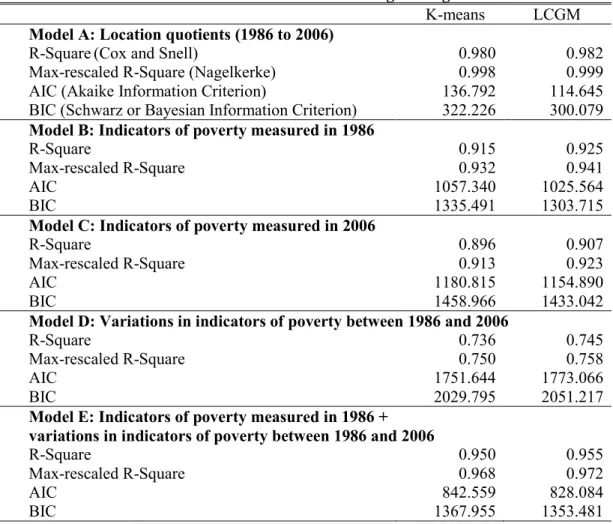
Results of multinomial logistic regressions further inform on which of the k-means and LCGM performs better in identifying trajectories of neighbourhood change. To do so, we only present fit statistics from MLR models (R-Square, max-rescaled R-Square, AIC and BIC); results are reported in the Table 4. Model A examines how the location quotients measured at the five time points (and used for the classification) predict ‘belonging’ to a trajectory. Results show that LCGM very marginally outperformed k-means as shown by lowest AIC and BIC values. This indicates that LCGM might be more accurate in identifying groups of census tracts having followed similar trajectories of change over the period.
When other predictors of poverty were used to predict trajectories (models B to E), LCGM again seems to perform better than k-means. Yet the difference between models is again very modest. Indeed, as shown in Table 4, the R-Square of multinomial regression are very strong for both the k-means and LCGM models, given that the predictors of the models are known to be associated with poverty (excessive multicolinearity was not a problem in our models, as indicated by variance inflation factor values lower than 10 not reported here). R-Square values are essentially the same in all models (for example, R-Squares for model A are 0.915 for k-means and 0.925 for LCGM). However, except for the model D, all values of AIC and BIC are lower for the LCGM clustering.
18
Table 4. Model fit statistics from multinomial logistic regression models
K-means LCGM
Model A: Location quotients (1986 to 2006)
R-Square(Cox and Snell) 0.980 0.982
Max-rescaled R-Square (Nagelkerke) 0.998 0.999
AIC (Akaike Information Criterion) 136.792 114.645
BIC (Schwarz or Bayesian Information Criterion) 322.226 300.079
Model B: Indicators of poverty measured in 1986
R-Square 0.915 0.925
Max-rescaled R-Square 0.932 0.941
AIC 1057.340 1025.564
BIC 1335.491 1303.715
Model C: Indicators of poverty measured in 2006
R-Square 0.896 0.907
Max-rescaled R-Square 0.913 0.923
AIC 1180.815 1154.890
BIC 1458.966 1433.042
Model D: Variations in indicators of poverty between 1986 and 2006
R-Square 0.736 0.745
Max-rescaled R-Square 0.750 0.758
AIC 1751.644 1773.066
BIC 2029.795 2051.217
Model E: Indicators of poverty measured in 1986 + variations in indicators of poverty between 1986 and 2006
R-Square 0.950 0.955
Max-rescaled R-Square 0.968 0.972
AIC 842.559 828.084
BIC 1367.955 1353.481
Discussion and conclusion
The aim of this paper was to compare two clustering techniques, k-means clustering and latent class growth models, in order to better characterize trajectories of neighbourhood poverty over a period of twenty years. Thus, the main contribution of this paper to the study of neighbourhood change is methodological, contributing novel applications of statistical clustering techniques to longitudinal data at the area level. Findings showed that both k-means and LCGM techniques were successful in grouping census tracts characterized by similar trajectories of change in poverty levels between 1986 and 2006. As observed in other studies, different trajectories of neighbourhood change in the Montreal CMA were captured, including trajectories of high concentration of low-income population in inner city areas; suburban areas characterized by increasing concentration of poverty over the twenty-year period.
These results supports other studies reporting a suburbanization of poverty in some North American metropolitan areas (Cooke et al., 2006; Madden, 2003); the gentrification of certain central areas (Heisz et al., 2006; Ley, 1986, 1988; Walks et al., 2008) along the increase of poverty concentration in other parts of the central city during the last twenty years (Bourne, 1993; Madden, 2003). However, most census tracts are characterized by somewhat stable poverty levels over the period, either in terms of stable but high levels of poverty concentration, or stable but low representation of poverty. Yet, most studies of neighbourhood trajectories are mainly concerned with change, i.e. either increase or decrease in poverty levels. Nevertheless,
19 our study shows that some areas have been persistently experiencing high levels of poverty between 1986 and 2006, whereas in others, poverty levels are continuously lower compared to the CMA as a whole.
Overall, the results of the two cluster solutions were relatively similar. However, we found some discrepancies between the maps of trajectories of relative deprivation obtained by k-means and LCGM methods. For the census tracts located in the suburbs, the LCGM solution identified three stable trajectories with low poverty levels against two for the k-means. In the central areas, the LCGM solution grouped into one trajectory 45 census tracts characterized by a decline of poverty concentration as a result of a gentrification process. Nonetheless, these 45 census tracts are divided into two trajectories of decreasing poverty concentration in k-means solution. In other words, the LCGM cluster solution provided more details in the suburbs while the k-means provided more details in central areas.
Finally, results of the multinomial logistic regressions showed that LCGM marginally outperformed k-means clustering. Since nowadays the LCGM method is more complex to implement than k-means clustering, the k-means still appears to be a robust and relevant approach to estimate trajectories of neighbourhood change where the clustering variable is measured continuously (e.g. location quotients). It should be recalled, however, that the k-means clustering could only be applied on continuous or binary variables whereas LCGM allows the identification of trajectories using variables with a range of different distributions (continuous, ordinal, nominal, count and binomial). Moreover, with the LCGM, it is also possible to maximize trajectories as a function of external variables (such as the predictors examined here for their association with the trajectories). Consequently, the LCGM approach is promising given its broader application. For instance, LCGM could be used to identify trajectories of neighbourhood change based on a count variable or a qualitative variable. Future studies are needed to test applications of LCGM to model neighbourhood change.
References
Abbas O. A., 2008, "Comparisons between data clustering algorithms", The International Arab Journal of Information Technology, vol. 5, no 3, 320-325.
Andruff H., Carraro N., Thompson A., Gaudreau P., Louvet B., 2009, "Latent Class Growth Modelling: A Tutorial", Tutorials in Quantitative Methods for Psychology, vol. 5,11-24.
Apparicio P., Séguin A.-M., Leloup X., 2007, "Modélisation spatiale de la pauvreté à Montréal: Apport méthodologique de la régression géographiquement pondérée", The Canadian Geographer / Le Géographe canadien, vol. 51, no 4, 412-427.
Apparicio P., Séguin A. M., Riva M., 2012, "Identifying, mapping and modelling trajectories of poverty at the neighbourhood level: The case of Montréal, 1986-2006", Applied Geography,
Barnett T. A., Gauvin L., Craig C.-L., Katzmarzyk P. T., 2008, "Distinct trajectories of leisure time physical activity and predictors of trajectory class membership: a 22 year cohort study", International Journal of Behavioral Nutrition and Physical Activity, vol. 5:57,
Berry B. J. L., 1986, "Inner City Futures: An American Dilemma Revisited", Transactions of the Institute of British Geographers, vol. 5, no 1, 1-28.
Bourne L. S., 1993, "The myth and reality of gentrification: a commentary on emerging urban forms", Urban Studies, vol. 30, no 1, 183-189.
Brookmeyer K. A., Henrich C. C., 2009, "Disentangling adolescent pathways of sexual risk taking", Journal of Primary Prevention, vol. 30,677-696.
20 Bunting T. E., Filion P., 1988, "Introduction: the movement towards the post-industrial society and the changing role of the inner city", in Bunting T. E., Filion P. (eds), The changing Inner City, Waterloo, University of Waterloo, 1-24.
Calińskia T., Harabasza J., 2007, "A dendrite method for cluster analysis", Communications in Statistics, vol. 3, no 1, 1-27.
Clark W. A. V., 1987, "The Roepke Lecture in Economic Geography Urban Restructuring from a Demographic Perspective", Economic Geography, vol. 63, no 2, 103-125.
Collins L. N., Lanza S. T., 2009, Latent Class and Latent Transition Analysis: With Applications in the Social, Behavioral, and Health Sciences, Hoboken (New Jersey), John Wiley & Sons.
Cooke T., Marchant S., 2006, "The changing intrametropolitan location of high-poverty neighbourhoods in the US, 1990-2000", Urban Studies, vol. 43, no 11, 1971-1989.
Duncan T. E., Duncan S. E., Strycker L. A., 2009, An Introduction to Latent Variable Growth Curve Modeling: Concepts, Issues, and Applications, Mahwah (New Jersey), Lawrence Erlbaum Associates.
Everitt B., Landau S., Leese M., 2001, Cluster Analysis, London, Heineman Educational Books.
Friedman M., Kandel A., 1998, Introduction to pattern recognition : Statistical, structural, neural and fuzzy logic approaches, Singapore, World Scientific Publishing Company.
Heisz A., McLeod L.,2006, Low-income in Census Metropolitan Areas, 1980-2000. Ottawa, Minister of Industry.
Jain A. K., 2007, "Data clustering: 50 years beyond K-means", Pattern Recognition Letters, vol. 31, no 8, 651–666.
Jargowsky P., 2003, Stunning Progress, bidden problems: The dramatic decline of concentrated poverty in the 1990’s, Washington D.C., The Brookings Institution.
Jones B. L., Nagin D. S., 2007, "Advances in group-based trajectory modeling and an SAS procedure for estimating them", Sociological Methods & Research, vol. 35, no 4, 542-571.
Kaufman L., Rousseeuw P. J., 2005, Finding groups in data: An introduction to cluster analysis, Hoboken, NJ, Wiley series in Probability and Statistics.
Kitchen P., Williams A., 2009, "Measuring neighborhood social change in Saskatoon, Canada: A geographic analysis", Urban Geography, vol. 30, no 3, 261-288.
Lee S., 2011, "Analyzing intra-metropolitan poverty differentiation: causes and consequences of poverty expansion to suburbs in the metropolitan Atlanta region", Annals of Regional Science, vol. 46, no 1, 37-57.
Lee S., Leigh N. G., 2007, "Intrametropolitan spatial differentiation and decline of inner-ring suburbs - A comparison of four US metropolitan areas", Journal of Planning Education and Research, vol. 27, no 2, 146-164.
Ley D., 1986, "Alternative Explanations for Inner-City Gentrification: A Canadian Assessment", Annals of the Association of American Geographers, vol. 76, no 4, 521-535.
Ley D., 1988, "Social upgrading in six Canadian inner cities", The Canadian Geographer / Le Géographe canadien, vol. 32, no 1, 31-45.
Madden J. F., 2003, "The changing spatial concentration of income and poverty among suburbs of large US Metropolitan areas", Urban Studies, vol. 40, no 3, 481-503.
Magidson J., Vermunt J. K., 2002, "Latent class models for clustering: A comparison with K-means", Canadian Journal of Marketing Research, vol. 20,37-44.
21 McConville S., Ong P., 2003, The trajectory of poor neighborhoods in Southern California, 1970-2000, Washington, DC, Center on Urban and Metropolitan Policy, The Brookings Institution.
Mikelbank B. A., 2004, "A typology of U.S. suburban places", Housing Policy Debate, vol. 15,935-964.
Mikelbank B. A., 2006, "Local Growth Suburbs: Investigating Change within the Metropolitan Context", Opolis, vol. 2, no 1, 1-15.
Mikelbank B. A., 2011, "Neighborhood déjà Vu: Classification in metropolitan Cleveland, 1970-2000", Urban Geography, vol. 32, no 3, 317-333.
Milligan G. W., Cooper M. C., 1985, "An examination of procedures for determining the number of clusters in a data set", Psychometrika, vol. 50, no 2, 159-179.
Muthén & Muthén Mplus. Los Angeles, CA, USA.
Nagin D. S., 2005, Group-based modelling of development, Cambridge, MA, Harvard University Press.
Pearson A. L., Apparicio P., Riva M., 2013, "Cumulative disadvantage? Exploring relationships between neighbourhood deprivation trends (1991 to 2006) and mortality in New Zealand", International Journal of Health Geographics, vol. 12, no 38, 1-8.
Reibel M., Regelson M., 2007, "Quantifying neighborhood racial and ethnic transition clusters in multiethnic cities", Urban Geography, vol. 28, no 4, 361-376.
Reibel M., Regelson M., 2011, "Neighborhood racial and ethnic change: the time dimension in segregation", Urban Geography, vol. 32, no 3, 360-380.
Riva M., Curtis S. E., 2012, "Long-term local area employment rates as predictors of individual mortality and morbidity: A prospective study in England, spanning more than two decades", Journal of Epidemiology and Community Health,
Rose D., 1984, "Rethinking gentrification beyond the uneven development of marxist urban theory", Environment and Planning D : Society and Space, vol. 12, no 1, 47-74.
Sarle W. S., 1983, Cubic Clustering Criterion, Cary, NC, SAS Institute Inc. SAS Institute Inc SAS version 9.2. Cary, NC, USA.
Séguin A.-M., Apparicio P., Riva M., 2012, "The Impact of geographical scale in identifying areas as possible sites for area-based interventions to tackle poverty: the case of Montréal", Applied Spatial Analysis and Policy, vol. 5, no 3, 231-251.
Shearmur R., Doloreux D., 2008, "Urban hierarchy or local buzz? high-order producer service and (or) knowledge-intensive business service location in Canada, 1991-2001", Professional Geographer, vol. 60, no 3, 333-355.
Shearmur R., Motte B., 2009, "Weak ties that bind: Do commutes bind Montreal's central and suburban economies?", Urban Affairs Review, vol. 44, no 4, 490-524.
Short J. R., Hanlon B., Vicino T. J., 2007, "The decline of inner suburbs: The new suburban gothic in the United States", Geography Compass, vol. 1/3,641-656.
Statistical Innovations Latent GOLD® 4.5. Belmont, MA, USA.
Statistics Canada, 2007, Montréal, Quebec (Code462) (table). 2006 Community Profiles. 2006 Census, Ottawa, Statistics Canada Catalogue no. 92-591-XWE.
Statistics Canada, 2011, Low Income Lines, 2009-2010, Ottawa, Minister of Industry (Canada). Tibshirani R., Walther G., Hastie T., 2001, "Estimation of number of clusters in a data set via the
gap statistic", Journal of the Royal Statistical Society: Series B, vol. 63, no 2, 411-423.
Van Kempen R., Murie A., 2009, "The new divided city: changing patterns in European cities", Tijdschrift voor Economische en Sociale Geografie, vol. 100, no 4, 377-398.
22 Vicino T., Hanlon B., Short J., 2011, "A typology of urban immigrant neighborhoods", Urban
Geography, vol. 32, no 3, 383-405.
Vicino T. J., 2008, "The spatial transformation of first-tier suburbs, 1970 to 2000: The case of metropolitan Baltimore", Housing Policy Debate, vol. 19, no 3, 479-518.
Walks R. A., 2001, "The social ecology of the post-fordist/global city? Economic restructuring and socio-spatial polarisation in the Toronto urban region", Urban Studies, vol. 38, no 3,
407-447.
Walks R. A., Maaranen R., 2008, "Gentrification, social mix, and social polarization: Testing the linkages in large Canadian cities", Urban Geography, vol. 29, no 4, 293-326.