Any correspondence concerning this service should be sent to the repository
administrator:
[email protected]
O
pen
A
rchive
T
OULOUSE
A
rchive
O
uverte (
OATAO
)
OATAO is an open access repository that collects the work of Toulouse researchers and
makes it freely available over the web where possible.
This is an author-deposited version published in:
http://oatao.univ-toulouse.fr/
Eprints ID: 16598
To cite this version:
T'Hooft, Jorrit and Lesire, Charles and Ponzoni Carvalho Chanel,
Caroline Online Proactive Planning with Multiple Hypotheses. (2016) In: 8th European
Starting AI Researcher Symposium (STAIRS), 26 August 2016 - 2 September 2016 (The
Hague, Holland, Netherlands).
Online Proactive Planning with Multiple
Hypotheses
Jorrit T’HOOFTa,1Charles LESIREaand Caroline P. CARVALHO CHANELb
aOnera – The French Aerospace Lab, France
bISAE-SUPAERO – Institut Sup´erieur de l’A´eronautique et de l’Espace, France
Abstract.
In order to enhance the behavior of autonomous service robots, we are explor-ing multiple paradigms for their plannexplor-ing and execution strategy (the way of in-terleaving the planning, selection and execution of actions). In this paper we fo-cus on continuous proactive planning with multiple hypotheses in order to continu-ously generate multiple solution-plans from which an action can be selected when appropriate. To illustrate the concepts, we develop how it could be used for au-tonomous navigation in dynamic environments, and analyze the tests we realized with several instantiations. We also discuss several aspects and concerns about the proposed strategy, and how integrating more semantic information could enhance the capabilities of service robots for real-world applications.
Keywords. Online Planning and Execution, Proactive Planning with Multiple Hypotheses, Planning under Uncertainty, Semantic Knowledge for Robotics
1. Introduction
In the near future we would like autonomous service robots able to accomplish com-plex missions in real environments. Such missions include human assistance, surveil-lance of infrastructure, search and rescue, and dangerous work. Real environments on the other hand are often dynamic, unstructured, open, unknown and only partially observ-able, which further complicates the execution of the already complex missions. In such context, it is impossible to precompute plans or policies able to cope with all unexpected events and unpredictable changes in the environment. Therefore, service robots need to plan and manage their actions online, which requires to take into account the following aspects:
Planning and execution strategy: The planning and execution strategy is the way of interleaving the planning, selection and execution of actions. Depending on the applica-tion, one strategy may be better suited than another. – In [1,2], the authors call for more research on the problems that arise when endeavoring to integrate acting with planning. Default behavior: A valid plan to reach some goal is not always available, e.g. when no plan has been computed yet, or the available plan is invalidated. In such situations the robot should execute “default” actions to ensure the integrity of itself and/or its
ronment. Such default behavior may be precomputed or obtained by fast (sub-optimal) planning. – In [3] for example, an emergency maneuver library is used to guarantee the safety of a robot.
Reactivity: The system must remain reactive, which imposes constraints on the soft-ware architecture. For example, the planning process may not block the rest of the sys-tem, s.t. when an unexpected event occurs the robot is still able to correctly adapt its behavior. – An overview of commonly used robotic architectures can be found in [4].
In order to enhance the behavior of service robots, we are exploring multiple paradigms for the planning and execution strategy. In this paper we focus on continuous proactive planning with multiple hypothesesin order to continuously generate multiple solution-plans from which an action can potentially be selected when required. In Sec. 2 we discuss a selection of existing planning and execution strategies to give some insight. In Sec. 3 we develop the main concepts of our continuous proactive planning with multi-ple hypothesesstrategy. Sec. 4 gives a high-level algorithm to show how such strategies can be implemented. To illustrate the concepts, we present in Sec. 5 how proactive plan-ning with multiple hypothesescould be used for autonomous navigation in dynamic envi-ronments, and analyze the tests we realized with several instantiations. In Sec. 6 we dis-cuss several aspects and concerns about the proposed strategy, as well as how integrating more semantic information could enhance the capabilities of service robots.
2. Existing Online Planning and Execution Paradigms
In online planning and execution paradigms, replanning can be triggered in order to adapt to changes in the environment or unexpected events. When replanning is triggered one can choose to replan from scratch or to repair the previous plan. A number of algorithms exist for repairing the previous plan [5], among which many are based on D* [6,7] which is able to propagate changes in its data-structures. However, depending on the applica-tion, it can be difficult to track those changes and a single change can invalidate a large part of the underlying graph, in which case it can be preferable to just replan from scratch with a faster algorithm (e.g with A* [8]).
The following selection of planning and execution strategies is meant to give some insight, but is in no way exhaustive.
Plan-Replan: A basic but commonly used planning and execution strategy is the plan-replanstrategy: The robot computes a plan that achieves the goal under some constraints based on the available information. During this time, the robot executes its default be-havior. Once a plan is available, the robot executes the actions of the plan as long as the plan remains valid. If at some moment the plan is invalidated, the execution is inter-rupted and replanning is triggered. The process repeats until goal completion. – In [9] this type of planning and execution strategy allowed a robot to complete 26.2 miles of autonomous navigation in a real office environment. Other approaches have proposed to take into account uncertainty directly in the planning model to reduce possible faults at execution. FF-Replan [10] for example transforms a probabilistic description of the environment into deterministic problems, computes a deterministic plan and executes it until an unexpected state occurs, in which case partial replanning is triggered.
Continuous Planning: The difference with plan-replan is that continuous planning tries to integrate observed discrepancies (e.g. changes in the environment), during the execution of a plan, to avoid that the available plan becomes invalid or sub-optimal. For this, during the execution of actions, replanning is triggered (periodically or when changes are observed) with the latest information available. The main advantages are: (1) As long as discrepancies can be integrated in time and the resulting plan remains valid, the use of default behavior can be avoided. (2) By continuous planning with the latest available information, the robot can take advantage of opportunities that occur during the execution, e.g. changes in the environment can create shortcuts that weren’t available be-fore. – In [11] the authors present a method for path planning in dynamic environments able to repair the previous plan in an anytime fashion. In [12], while the robot is navigat-ing, replanning is triggered during each action, to solve a reduced Partially Observable Markov Decision Process (POMDP) with the latest information available. If the action succeeds, the next action can be selected immediately. Otherwise, the robot pauses and the planner is rerun.
3. Continuous Proactive Planning with Multiple Hypotheses: Concepts 3.1. Proactive Planning
While continuous planning (as we described it in Sec. 2) often improves the behavior of the robot in dynamic environments, it lacks proactivity in the sense of anticipating future situations. By only planning with the latest available information it is often one step behind due to the duration needed for the planning. For example, no valid plan is available when a new action must be selected, if a change in the environment invalidates the current plan just before the selection, or when the search for a new solution takes too much time. The more the environment is dynamic and complex, the more this situation is likely to occur, and thus the more default actions will be executed because no valid plan is available. The use of many default actions (such as immobilizing the robot) may cause the robot to behave strangely for a human observer which is why we prefer to avoid this. In order to improve the continuous planning strategy in such situations, we propose to plan in a proactive manner for multiple hypotheses (which can correspond to predictable future situations) in order to generate multiple solution-plans from which an appropriate action can often be selected, depending on the actual encountered situation. For example, if it is known where obstacles may appear in the surrounding of the robot, the robot can anticipate these situations by searching for solutions in a proactive manner (before such an obstacle appears). Then, when an obstacle actually does appear, it is likely that a valid plan is already available, and the robot just has to select a new action from (one of) the valid plan(s). – In [13] an anticipatory online planning algorithm is presented for the problem in which additional goals may arrive while plans for previous goals are still executing. It samples possible futures according to their distribution and than solves each sampled future with a fast deterministic planner. While this approach, which has many ideas in common with ours, is very specific to a particular kind of applications, our approach is more generic and could easily be instantiated to behave the same.
3.2. Hypotheses
What we call a hypothesis is a collection of information in order to generate a corre-sponding type of solution-plan. It can take into account arbitrary information considered useful for the kind of solution one wants to generate with it, such as: constraints on the search space, a particular configuration or initialization, etc. For example, the hypothe-ses anticipating the appearing of obstacles could include a zone where obstacles can oc-cur, initialize the search with a previous plan, and restrict the search space within some range around that previous plan. The corresponding solution, if one is found, would be a solution “close” to the previous plan and avoiding the selected zone.
3.3. Using One or Multiple Planners
While the multiple hypothesis paradigm can be used with a single planning algorithm (like most existing paradigms), it proposes to select the appropriate planner(s) for each instantiated hypothesis. This can be interesting for multiple reasons: a planner can be more suited than another for a particular hypothesis (e.g. ability to deal with uncertain-ties, solving duration, optimality guarantees); one can also choose to solve a hypothesis with different planners to obtain different plans for the same constraints.
3.4. Tackling (some) Uncertainties with Multiple Hypotheses
Planning algorithms able to cope with uncertainties are often to slow to be usable for on-line planning if they are instantiated with all the possible uncertainties for the complete mission. With the multiple hypotheses paradigm, because it instantiates the hypotheses online, it is possible to generate solution-plans taking into account only a subset of the uncertainties to speed up the search (e.g. with a reduced MDP). This however still re-quests to have an accurate representation for the remaining uncertainties involved. An-other way to take into account (some) uncertainties, without the need to quantify them, is to proactively solve for (some of) the possible future situations separately.
4. Continuous Proactive Planning with Multiple Hypotheses: Algorithm
To guarantee the reactivity of the system (see Sec. 1), multiple threads are running in parallel: A supervising thread, described in Alg. 1, is in charge of the planning and ex-ecution strategy, and drives the other threads for planning, executing actions, and gath-ering information, in a non blocking way. The proposed algorithm was designed for im-plementing the continuous proactive planning with multiple hypotheses strategy, but can also be used for implementing the other strategies. The presented version (used for the tests) shows the principles when planning is done for one hypothesis at a time.
Algorithm 1 is a loop. First, it updates the data structures (line 2). Then, it ensures that the robot executes the most appropriate action (lines 3 to 8). The selected action can for example be the first action of the best valid plan available, or the appropriate “default” action if no valid plan is available. Finally, it manages the planning part (lines 9 to 17).
Algorithm 1 behaves differently according to its instantiation, more precisely to: the way the action to execute is selected, the selection of the hypotheses to plan for and the scheduling of the planning episodes. Depending on how this is done it can even be used for implementing the continuous planning and the plan-replan strategies as showed next.
Algorithm 1 Continuous proactive planning with multiple hypotheses
1: loop
2: update current goal, current state, planning results (if any)
3: if no action executing then
4: select most appropriate action to execute; launch selected action
5: else
6: verify if the executing action is still the most appropriate
7: if a more appropriate action is available then
8: stop the execution of current action; launch new most appropriate action
9: if currently planning then
10: if the hypothesis for which we are planning is still coherent then
11: continue planning
12: else
13: stop the corresponding planning algorithm
14: if currently not planning then
15: if hypothesis left to explore then
16: h← select hypothesis to plan for; select planning algorithm for h
17: create planning algorithm input for h; launch the planning algorithm for h
For the Plan-Replan Strategy:
Selection of the action to execute: Only one plan is stored in the “planning results”. If the plan is valid from the current state to the goal, the action to apply is selected from the available plan, otherwise the action corresponding to the default behavior is selected. Selection of the hypothesis to plan for and scheduling of the planning episodes: There is only one hypothesis, corresponding to the observed situation. Replanning is triggered only when no valid plan is available. The planner is not interrupted before it finishes. If a solution is found, it replaces the previous plan.
For the Continuous Planning Strategy:
Selection of the action to execute: The same as for the plan-replan strategy.
Selection of the hypothesis to plan for and scheduling of the planning episodes: There is only one hypothesis, corresponding to the observed situation. Replanning is triggered periodically (e.g. each time an action is launched) or when changes are observed. If the previous search did not finish yet when replanning is triggered, depending on the planner used, it can be updated (e.g. if a D* planner is used) or interrupted (e.g. if an A* planner is used). If a solution is found, it replaces the previous plan.
5. Application to Autonomous Navigation in Dynamic Environments
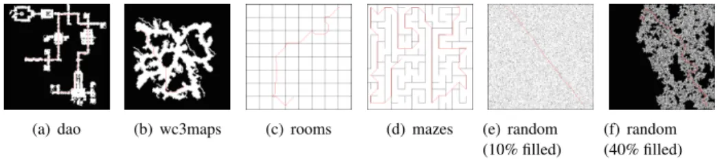
To illustrate and evaluate the proposed concepts, we tested several instantiations of the continuous proactive planning with multiple hypotheses strategy, in the context of au-tonomous navigation in dynamic environments, and compared the results w.r.t the plan-replan and continuous planning strategies. The goal was to use multiple hypothesis in order to reduce the number of default actions launched and the durations of the missions. For generating our simulated test conditions, we started by selecting 6 missions from the benchmarks for grid-based path-finding [14]. Each one was selected from a different category (dao, wc3maps, rooms, mazes, random (10%), random (40%)), and includes
a start and a goal position, along with a map (2D occupancy-grid of about 512 ∗ 512 grid-cells of 1 ∗ 1m), which we used for the static part of the environment (see Fig. 1).
(a) dao (b) wc3maps (c) rooms (d) mazes (e) random (10% filled)
(f) random (40% filled) Figure 1. The maps used for the tests (with in red the initial plan).
Starting at the center of a free grid-cell, the robot can execute nine possible actions. The eight “normal” actions correspond to the displacement of the robot to the center of an adjacent grid-cell, following a straight line-segment at constant velocity (2m · s−1for the tests). Such an action is valid only if the corresponding line-segment does not encounter an obstacle (occupied grid-cell). The ninth action corresponds to immobilizing the robot at its current position and is only used as default behavior (it is always valid).
A plan is a path consisting of a sequence of “normal” actions, leading the robot to its goal position. For computing such plans, we dispose of 2 deterministic planners: one based on A* and one based on D* Lite. They take as input a start and goal position, along with a static occupancy-grid representation of the environment, and return a plan that minimizes the path length for the given static environment. As the robot moves at constant speed, this also optimizes the duration for reaching the goal if the environment remains unchanged. For replanning from scratch, A* is much faster than D* Lite. On the other hand, as long as the goal remains the same, D* Lite is able to repair a previous plan, while A* must always replan from scratch. For our tests, most of the time, it was much faster to repair the previous plan with D* Lite than replanning from scratch with A*, which is not necessarily the case for real applications (see Sec. 2).
In order to evaluate how the different strategies behave, when dynamic obstacles invalidate the plan being executed, we choose to add obstacles on the path followed by the robot during the simulations. For a real-world application, the robot can only update the part of its environment representation it observes, which is why we choose to add “dynamic” obstacles only on the first part of the followed path. After each executed action, an obstacle may appear on the followed path with probability Pobstacle. The
grid-cell the obstacle should occupy is randomly chosen with a uniform distribution, selecting one of the next nine grid-cells crossed by the followed path. At the same time, each previously added obstacle may also be removed with the same probability. To simulate environments with different dynamics, we realized the tests for Pobstacle∈ {0.2, 0.5, 0.8}.
In the real world, executing a “default” action can take longer than just the duration needed for replanning a new valid path, e.g. instead of being able to “instantaneous” stop or evolve at constant speed it can require a minimum duration to stabilize the robot. Therefore, we will compare the results for the two cases: (A) the duration of a ”default” action equals the (re)planning duration; (B) the ”default” action has a minimum duration of 0.5s (chosen to correspond to the minimum duration of a “normal” action).
5.1. Explored Types of Hypotheses and Instantiated Configurations
In order to instantiate the proposed algorithm for the different strategies, we need to define the hypotheses to use.
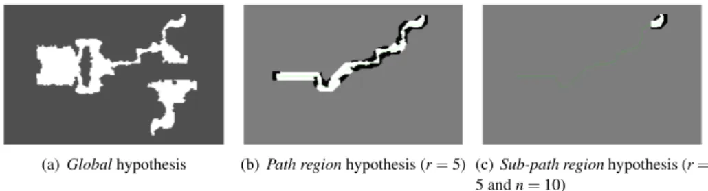
Global Hypothesis: What we call the global hypothesis corresponds to what is most often used for solving a planning problem. It consists of giving the planning algorithm the complete representation of the environment and letting it compute a global solution to the goal from a given source state. For our tests it corresponds to giving the complete occupancy-grid representation of the environment, and the source and goal position for the robot. The advantage of this hypothesis is that the solutions are global and can thus be globally optimal depending on the planning algorithm used. The main disadvantage is that finding a global (optimal) solution is often computationally expensive and thus often slow. Figure 2(a) shows an example of an occupancy-grid representation of a global hypothesis.
Path Region and Sub-Path Region Hypotheses: To speed up the search, we created the following hypotheses restricting the search space.
The path region hypothesis supposes a path already exists and limits the search space for the planner in some range around it. For our tests, it consists of taking into account only the region around the followed path, considering the rest of the space as obstacles (unreachable). The range is parameterized with r, corresponding to the number of grid-cells taken into account around the path. The main advantages are: (1) When a solution is found it is a global solution and thus the robot will not get stuck in a local optimum. (2) Often the search is largely sped up, for example in environments such as mazes. One drawback is that it does not take into that only part of the environment representation has been updated since the existing path was generated. Once outside that region, it is likely that the new path, in the unchanged but restricted environment, will converge to the existing path, and the same solution will be computed over again consuming time for nothing. A second drawback is that by only looking for solutions locally around a previous path it can easily discard opportunities that occur during execution (e.g. a door that opens) and thus losing its global optimality. Figure 2(b) shows an example of an occupancy-grid representation of the path region hypothesis with r = 5.
The sub-path region hypothesis is a solution for the first drawback mentioned for the path regionhypothesis. It restricts the search space even more by taking into account only the first part of the existing path. The last state of this sub-path becomes the sub-goal. The path-region hypothesis is constructed for the sub-path and is solved for reaching the sub-goal. And finally, a global path to the real goal is reconstructed by combining the new solution to the sub-goal, and the existing path for the remaining part. It has the same range parameter r as the path region hypothesis, and the sub-goal can be expressed with a parameter n s.t. the sub-goal corresponds to the state: f irst state o f selected path + n (state x + n means the state reached after applying the first n actions of the followed path from state x). The main advantage is of course the speed up compared to the path regionhypothesis. Figure 2(c) shows an example of an occupancy-grid representation of the sub-path region hypothesis with r = 5 and n = 10.
With the global and sub-path region hypotheses we instantiated the following con-figurations.
(a) Global hypothesis (b) Path region hypothesis (r = 5) (c) Sub-path region hypothesis (r = 5 and n = 10)
Figure 2. Occupancy-grid representations of hypotheses. White represents free space, gray occupied space.
Instantiations of Plan-Replan:
PR-A: This is the simplest configuration. Replanning is only triggered when no valid plan is available. The search is done with the A* planner (always from scratch). The only hypothesis used is the global hypothesis.
PR-D: Similar to PR-A, but the (re)planning is done with the D* Lite planner (able to adapt its previous plan).
Instantiation of Continuous Planning:
CP-D: Replanning is triggered each time a new action is launched. The hypothesis and planner are the same as for PR-D.
Instantiations of Continuous Proactive Planning with Multiple (10) Hypotheses: In order to instantiate the additional hypotheses, the following configurations suppose some minimal semantic information is available about where obstacles can appear. (For our tests this information was directly available from the simulations, but for a real ap-plication it should be provided by another component of the system.)
CPP-1: This configuration uses 10 hypotheses. Each time a “normal” action is launched, it first tries to solve the global hypothesis just like the continuous planning strategy. Then, while there is time left until the action finishes, it sequentially plans for sub-path regionhypotheses with A*. Each sub-path region hypothesis has a range pa-rameter r = 5, but the sub-goal papa-rameter n takes respectively the values 2 to 10. Here semantic knowledge is used to select the sub-goals s.t. they correspond to the positions on the previous path just after the places where dynamic obstacles can appear. These hy-potheses locally optimize the path to the selected sub-goals with the freshest information available, but without considering that dynamic obstacles can appear or disappear. When a “default” action is launched instead, it only tries to solve the global hypothesis. CPP-2: This is almost the same as CPP-1, but for the sub-path region hypotheses we also add a (hypothetical) obstacle in the corresponding occupancy-grid on the selected path just before the sub-goals. These hypotheses are thus anticipating the apparition of dynamic obstacles on the followed path, but without taking into account that obstacles can also disappear. Here even more semantic knowledge is used to predict the positions and sizes of future obstacles.
CPP-3: This final configuration has the same principle of CPP-2, i.e. it tries to antic-ipate the apparition of dynamic obstacles on the followed path (still without taking into account that obstacles can also disappear). But as D* Lite can repair a plan fast for a globalhypothesis, all hypotheses are global, where for the last 9 hypotheses a predicted obstacle is taken into account just like for CPP-2.
5.2. Test Results
Each mission was realized 30 times with each configuration, and for Pobstacle ∈ {0.2, 0.5, 0.8} to simulate increasing dynamics.
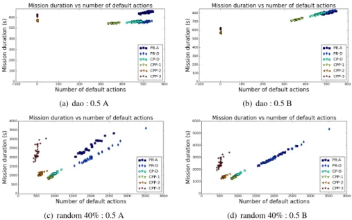
Except for CPP-3, the characteristics of the results w.r.t. the different values of Pobstaclewere the same, but emphasized with the increase of dynamics. Figure 3 shows
the mission durations against the number of default actions launched during the missions, for Pobstacle= 0.5. The results for the tests based on the first five maps had the same
char-acteristics and can be observed in Fig.3(a) and 3(b), representing the results for the first environment (“dao”). The results for the tests based on the sixth environment (“random (40% filled)”) are shown in Fig. 3(c) and 3(d).
As expected, for the plan-replan configurations, PR-D was able to adapt its previ-ous plan faster than PR-A which replanned from scratch, and the continuprevi-ous planning configuration CP-D executed less “default” actions than the plan-replan configurations. For the configurations with multiple hypotheses, when a “normal” action was executed, they were almost always able to finish the search for the 10 hypotheses in time (before the action finished), which means that the planners were efficient enough to return the solutions before they became obsolete.
(a) dao : 0.5 A (b) dao : 0.5 B
(c) random 40% : 0.5 A (d) random 40% : 0.5 B
Figure 3. The mission durations against the number of default actions launched during the missions, for Pobstacle= 0.5 (indicated with 0.5). Above: for the environment from “dao”; Under: for the environment from
“random (40% filled)”. Left: without minimum duration for the default actions (indicated with the suffix “A”); Right: with minimum duration of 0.5 seconds for the default actions (indicated with the suffix “B”).
For the first five environments:
Case A: When the duration of a “default” action equals the (re)planning duration: The strategy that minimized the mission durations is CPP-1 (slightly faster than the con-tinuous planningstrategy CP-D).
Both CPP-2 and CPP-3 were able to avoid almost all default behavior, but CPP-2 realized the missions faster than CPP-3 (about as fast as the continuous planning strategy CP-D).
Case B: When a “default” action has a minimum duration of 0.5s:
Because most of the time, replanning a new valid path was faster than 0.5s, the impact of reducing the number of launched “default” actions is much more noticeable here. There-fore, CPP-2 became also the fastest of all strategies (about 25% faster than the continuous planningstrategy CP-D) and became clearly the best of the tested configurations.
For this kind of environments, the selected hypotheses of CPP-2 were appropriate to reduce the execution of default behavior. This is because most of the time, it was able to find local solutions avoiding the appearing obstacles (in the selected range around the previous path).
For the sixth environment (“random (40% filled)”):
Case A: When the duration of a “default” action equals the (re)planning duration: The strategy that minimized the mission durations is still CPP-1.
CPP-2 was able to avoid more default behavior, and had still about the same mission durations as the continuous planning strategy CP-D.
CPP-3 had different results than expected. We thought that by anticipating the apparition of obstacles and searching globally for solutions, it would continue to improve the mis-sion durations. But it was actually the configuration that executed the longest trajectories to reach the goal. This is probably because it often found solutions that differed globally from the previous plan, changing radically the followed path, and when “dynamic” ob-stacles appeared or disappeared it doubled back. This was catastrophic for this sixth en-vironment with the highest dynamics (Pobstacle= 0.8, not shown on the figures), where it
doubled back so often that it barely progressed to the goal. For Pobstacle= 0.8, the fastest
execution took more than 15 times the duration of the other strategies, and the slowest more than 30 times. CPP-1 and CPP-2 suffered much less from this phenomenon because their hypotheses “stabilized” the updated plan around the previous path, and when this was not possible they replanned with the latest changes updated.
Case B: When a “default” action has a minimum duration of 0.5s:
The reduction of default behavior realized with CPP-2 made it about as fast as CPP-1 (slightly faster than the continuous planning strategy CP-D).
For this kind of environments, the hypotheses of CPP-2 were less appropriate to re-duce the execution of default behavior. This is because often, no local solutions avoiding the appearing obstacles existed (in the selected range around the previous path).
What we can conclude from the tests is that proactive planning with multiple hy-pothesesmay be able to improve the performances compared to commonly used strate-gies. As proof of concept, for our tests: If the priority is to complete the mission in mini-mum duration, CPP-1 performed the best when the duration of a “default” action equals the (re)planning duration; or CPP-2 if a “default” action has a minimum duration of 0.5s. If instead the priority is to avoid default behavior, CPP-2 can be preferred for both cases. On the other hand, the hypotheses to plan for and the actions to execute must be selected carefully, otherwise unexpected behavior may appear (such as for CPP-3).
6. Discussion
6.1. Optimality Concerns
The presented strategy on itself does not restrict or enforce optimality guarantees. The optimality aspects depend more on the instantiated hypotheses, the selected planners, and the function that selects the “most appropriate” action to execute depending on the con-text. Guaranteeing some optimality for real applications in unpredictable environments is not an easy task, and one should also know what such a guarantee really means. For example, (PO)MDP solvers optimize the expected reward (thus return the best policy for infinite executions), but does this really makes much sense for a mission that is exe-cuted only once? For our tests, our planners optimized the length of the path to the goal, but they only guarantee to return the shortest path for the static environment description given as input. If the actual environment changes during the execution, the guarantee is lost. This is why we prefer to search for “good” solutions in the sense of feasible, accept-able and appropriate, instead of guaranteed optimal solutions which we don’t know how to define or obtain in our context.
6.2. Critical Aspects
For obtaining a “good” set of solution-plans with the continuous proactive planning with multiple hypotheses strategy, some aspects are critical: (1) Obviously, the choice and construction of the hypotheses to plan for are very important. We observed that the con-struction of interesting hypotheses is very difficult without enough semantic informa-tion on the environment. (2) The planning algorithm selected to solve for a hypothesis must be efficient enough to return a solution before the hypothesis becomes obsolete. (3) Selecting the appropriate action to execute must be done carefully.
6.3. Computational Overhead
One can be concerned about the computational overhead because, of course, solving for multiple hypotheses is more computational intensive than solving for one. Therefore, it is the role of the underlying function that indicates if there is a “hypothesis left to explore”, to return true only when appropriate. However, as the planning is done during the execution of actions, computational resource is often available.
6.4. Semantic Information
While the proactive planning with multiple hypotheses paradigm looks promising and natural for anticipating future situations, we observe that it critically needs semantic in-formation to be efficient. However, if enough semantic knowledge is available, the robot could largely enhance its capabilities, for example by inferring automatically: more in-teresteing hypotheses, taking into account that a person can let the robot pass, a chair can be moved, some places would better be avoided, etc.; which hypothesis to instantiate in which context; which planner to use for solving a particular hypothesis; how to create the right input for a planner and a hypothesis; how to schedule the planning episodes. (e.g.: for hypotheses with defferent time horizons, priorities, ...); and how to select the most appropriate action. Therefore, we are investigating tools for acquiring and manag-ing semantic information, such as the ones presented in [15,16,17].
7. Conclusion
We presented the continuous proactive planning with multiple hypotheses strategy. Its concept is to proactively plan for multiple hypotheses, during the execution of actions, to generate multiple solution-plans from which an appropriate action can be selected when required. To illustrate the concepts, we developed how it could be used for autonomous navigation in dynamic environments, and analyzed the test we realized with several in-stantiations. The proactive planning with multiple hypotheses paradigm looks promising and natural for anticipating future situations, but needs enough semantic information to be efficient. We also argued how integrating more semantic information could enhance the capabilities of service robots. Therefore we continue our work focusing on how this can be done effectively.
References
[1] D. S. Nau, M. Ghallab, and P. Traverso, “Blended Planning and Acting: Preliminary Approach, Research Challenges,” in AAAI 2015, (Austin, TX, USA), 2015.
[2] M. Ghallab, D. Nau, and P. Traverso, “The actor’s view of automated planning and acting: A position paper,” Artificial Intelligence, vol. 208, pp. 1–17, 2014.
[3] S. Arora, S. Choudhury, D. Althoff, and S. Scherer, “Emergency maneuver library-ensuring safe navi-gation in partially known environments,” in ICRA, (Seattle, WA, USA), 2015.
[4] D. Kortenkamp and R. Simmons, “Robotic systems architectures and programming,” in Springer Hand-book of Robotics, pp. 187–206, Springer, 2008.
[5] D. Ferguson, M. Likhachev, and A. Stentz, “A guide to heuristic-based path planning,” in ICAPS work-shop on Planning under uncertainty for autonomous systems, (Monterey, CA, USA), 2005.
[6] A. Stentz et al., “The Focussed D* Algorithm for Real-Time Replanning,” in IJCAI, (Quebec, Canada), 1995.
[7] S. Koenig and M. Likhachev, “Improved fast replanning for robot navigation in unknown terrain,” in ICRA, (Washington, DC, USA), 2002.
[8] P. E. Hart, N. J. Nilsson, and B. Raphael, “A formal basis for the heuristic determination of minimum cost paths,” IEEE Transactions on Systems Science and Cybernetics, vol. 4, no. 2, pp. 100–107, 1968. [9] E. Marder-Eppstein, E. Berger, T. Foote, B. P. Gerkey, and K. Konolige, “The Office Marathon: Robust
navigation in an indoor office environment,” in ICRA, (Anchorage, AK, USA), 2010.
[10] S. W. Yoon, A. Fern, and R. Givan, “FF-Replan: A baseline for probabilistic planning.,” in ICAPS 2007, (Providence, RI, USA), 2007.
[11] J. Van Den Berg, D. Ferguson, and J. Kuffner, “Anytime path planning and replanning in dynamic environments,” in ICRA 2006, (Orlando, FL, USA), 2006.
[12] B. Marthi, “Robust navigation execution by planning in belief space,” in RSS, (Sydney, Australia), 2012. [13] E. Burns, J. Benton, W. Ruml, S. W. Yoon, and M. B. Do, “Anticipatory on-line planning,” in ICAPS,
(S˜ao Paulo, Brazil), 2012.
[14] N. Sturtevant, “Benchmarks for Grid-Based Pathfinding,” Transactions on Computational Intelligence and AI in Games, vol. 4, no. 2, pp. 144 – 148, 2012.
[15] M. Beetz, F. B´alint-Bencz´edi, N. Blodow, D. Nyga, T. Wiedemeyer, and Z.-C. Marton, “RoboSherlock: Unstructured Information Processing for Robot Perception,” in ICRA, (Seattle, WA, USA), 2015. [16] M. Tenorth and M. Beetz, “Representations for robot knowledge in the KnowRob framework,” Artificial
Intelligence, In Press 2015.
[17] M. Beetz, L. M¨osenlechner, and M. Tenorth, “CRAM – A Cognitive Robot Abstract Machine for every-day manipulation in human environments,” in IROS, (Taipei, Taiwan), 2010.