HAL Id: hal-00822961
https://hal.archives-ouvertes.fr/hal-00822961
Submitted on 16 May 2013
HAL is a multi-disciplinary open access
archive for the deposit and dissemination of
sci-entific research documents, whether they are
pub-lished or not. The documents may come from
teaching and research institutions in France or
abroad, or from public or private research centers.
L’archive ouverte pluridisciplinaire HAL, est
destinée au dépôt et à la diffusion de documents
scientifiques de niveau recherche, publiés ou non,
émanant des établissements d’enseignement et de
recherche français ou étrangers, des laboratoires
publics ou privés.
PERIODIC BEHAVIORS IN COUNTABLE
CELLULAR SYSTEMS
Laurent Gaubert, Pascal Redou
To cite this version:
Laurent Gaubert, Pascal Redou. SYNCHRONIZATION OF ASYMPTOTICALLY PERIODIC
BE-HAVIORS IN COUNTABLE CELLULAR SYSTEMS. Journal of Nonlinear Systems and
Applica-tions, JNSA, 2010, 1 (1), pp.1-12. �hal-00822961�
SYNCHRONIZATION OF ASYMPTOTICALLY PERIODIC
BEHAVIORS IN COUNTABLE CELLULAR SYSTEMS
Laurent Gaubert and Pascal Redou
Abstract. We address the question of frequencies locking in coupled differential systems and of the existence of (component) quasi-periodic solutions of some kind of differential systems. These systems named “cellular systems”,are quite general as they deal with countable number of coupled systems in some general Banach spaces. Moreover, the inner dynamics of each subsystem does not have to be specified. We reach some general results about how the frequencies locking phenomenon is related to the structure of the coupling map, and therefore about the localization of a certain type of quasi-periodic solutions of differential systems that may be seen as cellular systems. This paper gives some explanations about how and why synchronized behaviors naturally occur in a wide variety of complex systems.
Keywords. Coupled systems, synchronization, frequencies lock-ing, quasi-periodic motions, differential systems, asymptotically pe-riodic.
1
Introduction
Synchronization is an extremely important and interest-ing emergent property of complex systems. The first ex-ample found in literature goes back to the 17th century with Christiaan Huygens’ work [11, 2]. This kind of emer-gent behavior can be found in artificial systems as well as in natural ones and at many scales (from cell to whole ecological systems). Biology abounds with periodic and synchronized phenomena and the work of Ilya Prigogine shows that such behaviors arise within specific conditions: a dissipative structure generally associated to a nonlinear dynamics [20]. Biological systems are open, they evolve far from thermodynamic equilibrium and are subject to numerous regulating processes, leading to highly nonlin-ear dynamics. Therefore periodic behaviors appnonlin-ear (with or without synchronization) at any scale [21]. More gen-erally, life itself is governed by circadian rhythms [9]. Those phenomena are as much attractive as they are often spectacular: from cicadia populations that appear spon-taneously every ten or thirteen years [10] or networks of heart cells that beat together [17] to huge swarms in which fireflies, gathered in a same tree, flash simultaneously [3].
∗Laurent Gaubert and Pascal Redou are with Centre Europ´een
de R´ealit´e Virtuelle, LISYC EA3883 UBO/ENIB, 25 rue Claude Chappe, 29280 Plouzan´e, France. E-mail: [email protected]
†Manuscript received April 19, 2009; revised January 11, 2010.
This synchronization phenomenon occupies a privileged position among emergent collective phenomena because of its various applications in neuroscience, ecology, earth Science, for instance [27, 25, 16], as well as in the field of coupled dynamical systems, especially through the notion of synchronization of chaotic systems [18, 7] and the study of coupled-oscillators [13]. This wide source of examples leads the field of research to be highly interdisciplinary, from pure theory to concrete applications and experimen-tations.
The classical concept of synchronization is related to the locking of the basic frequencies and instantaneous phases of regular oscillations. One of the most success-ful attempts to explore this emergent property is due to Kuramoto [14, 15]. As in Kuramoto’s work, those ques-tions are usually addressed by studying specific kinds of coupled systems (see for instance [5, 22, 8]). Using all the classical methods available in the field of dynamical systems, researchers study specific trajectories of those systems in order to get information on possible attract-ing synchronized state [28, 13, 22, 19, 8, 12].
The starting point of this work was the following ques-tion : “Why synchronizaques-tion is such a widely present phe-nomena ?” In order to give some mathematical answer to this question, the first step is to build a model of coupled systems that is biologically inspired. This is done in the second section where, after having described some basic material, we define what we name cellular systems and cellular coupler. If one would summarize the specificities of cellular systems, one could say that each cell (subsys-tem) of a cellular system receives information from the whole population (the coupled system) according to some constraints:
• a cell has access to linear transformations of all the
others cell’s states
• the way this information is gathered depends (not
linearly) on the cell’s state itself
In other words, a cell interprets its own environment via the states of the whole population and according to its own state.
It is a bit surprising that despite this model arises very naturally, it gives a good framework to address the main
question. Indeed, in the third section we expose a local-ization result concerning some periodic and asymptoti-cally periodic trajectories of cellular systems. It exhibits some links between the coupler properties and the struc-ture of periodic trajectories.
The fourth section gives some example of general re-sults that may be proved using the localization lemma. Moreover, it goes out of the scope of coupled systems as synchronization is strongly related to the more abstract field of dynamical systems. If one thinks about presence of regular attractors (in opposition with strange attrac-tors) in a differential system, one may for example classify those as:
• point attractor • limit cycle • limit torus
Those attractors can be related to coupled systems in an obvious way: roughly speaking, a point attractor may be seen as a solution of coupled systems for which each of the subsystems has a constant behavior. Similarly, a limit cycle may be thought as the situation where every subsystem oscillates, all frequencies among the whole system being locked. A limit torus is a similar situation which differs from the previous one by the fact that the frequencies are not locked (non commensurable periods of a quasi-periodic solution of the whole coupled system). Hence, the three previous cases may be translated into the coupled dynamical systems context:
• point attractor ↔ constant trajectories
• limit cycle ↔ periodic trajectories, locked frequencies • limit torus ↔ periodic trajectories, unlocked
fre-quencies
Therefore, we deduce some results about the localiza-tion of solulocaliza-tions of the third type, quasi-periodic solu-tions, using the point of view of coupled dynamical sys-tems. The results of this fourth section may help to un-derstand why the second case is the most observed in natural systems, which may be seen as coupled dynami-cal systems (many levels). Indeed, the section ends with a sketch of how the cellular systems point of view may be applied to a wide class of differential systems in order to systematically address those questions with algebraic tools.
2
Basic material and notations
As our model is inspired by cellular tissues, some terms clearly come from the vocabulary used to describe this kind of complex systems.
2.1
Model of population behavior
Here are the basic compounds and notations of our model: A population I is a countable set, so we may consider it as a subset I ⊂ N. Moreover, only the cardinality of
I matters, so I may be chosen as an interval of integers.
Elements of I are called cells.
We suppose that the systems we want to study are valued in some Banach spaces. Thus, for any i ∈ I, (Ei, k.ki) is a Banach space, and the state space of I is
the vector space S =Y
i∈I
Ei.
We will sometimes identify Ei with
Y j<i {0} × Ei× Y j>i {0} ⊂ S
and then consider it as a subspace of S (in case one the inequalities j < i or i < j is empty, this identification remains valid as the void product is the empty mapping). Moreover, S has a natural structure of module on RI,
given λ : I → R and x ∈ S, one may define λ.x as:
λ.x = (λ(i).xi)i∈I
We denote Sb the space of uniformly bounded states:
Sb=
½
x ∈ S, sup
i∈Ikxiki< ∞
¾
This subspace will sometimes be useful as, embodied with the norm kxk∞ = supi∈Ikxiki, it is a Banach
space, allowing the classic Picard-Lindel¨of theorem to be valid.
Given an interval Ω ⊂ R, a trajectory x of I is an element of C∞(Ω, S). Such an x is then described by a
family of smooth applications (xi)i∈I such that ∀i ∈ I:
xi: Ω −→ Ei
t 7−→ xi(t)
Each cell i is supposed to behave according to an autonomous differential system given by a vector field
Fi : Ei → Ei. Thus, given a family of functions {Fi}i∈I
we define the vector field FI on S:
FI: S −→ S
x 7−→ FI(x)
where, for any i ∈ I:
[FI(x)]i= Fi(xi)
A period on I is a map τ : I → R∗
+. A trajec-tory x is said to be component τ -periodic (CP(τ )) if for any i ∈ I, xi is τ (i)-periodic and non constant.
In that case, τ (i) is a period of the cell i. If τ is bounded, a CP(τ ) trajectory which is not (globally) pe-riodic is said to be component τ -quasi-pepe-riodic (CQP(τ )). A trajectory x is said to be asymptotically component
τ -periodic (aCP(τ )) if there exists y which is CP(τ ) and α which vanishes when t → +∞ such that
x = y + α
In a similar way we define an asymptotically component
τ -quasi-periodic trajectory (aCQP(τ ))
Remark 2.1. We stress the point that a period of a component periodic trajectory needs not to be a minimal period (τ (i) is not necessarily a generator of the group of periods of xi). Nevertheless, the definition of CP(τ )
trajectories avoids any trajectory which contains some constant component (none of the xi can be a constant
map) as they may be seen as degenerate (localized into an “hyperplane” of S).
We recall that a (finite) subset {τ1, . . . , τk} of R is said
to be rationally dependent if there exists some integers
l1, . . . , lk non all zero and such that:
l1τ1+ . . . + lkτk = 0
Thus there exists a unique lowest common multiple (lcm)
τ0for which there exists n1, . . . , nk such that:
n1τ1= . . . = nkτk= τ0
An infinite set of real numbers is said to be rationally dependent if any finite subset is rationally dependent.
Now, any period τ on I defines an equivalence relation on I as:
i ∼ j ⇔τ {τ (i), τ (j)} is a dependent set
Hence we may consider the partition I(τ ) of I into equiv-alence classes (K countable):
I/τ = {Ik}k∈K
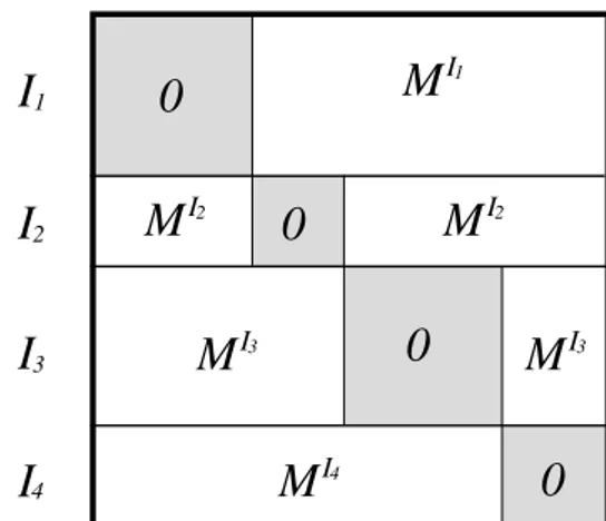
Let M = (mij)(i,j)∈I2 be a matrix indexed on I2, if J = {I1, ..., IK} is a partition of I, we define M/J as
the projection of M on the space of matrices with null coefficients on the I2 k (see figure 1): M/J = [(M/J)ij](i,j)∈I2 with (M/J)ij= ½ 0 if (i, j) ∈ I2 1∪ . . . ∪ IK2 mij if not
If τ is a period on I, we will write M/τ instead of
M/(I/τ ).
I
1I
2I
3I
4 IM
1 IM
2 IM
2 IM
3M
I3 IM
40
0
0
0
Figure 1: Projection of a matrix according to a partition of I.
2.2
Cellular coupler and cellular systems
In this section we build what we call cellular systems by means of cellular coupler. Most of the works in the field of synchronization deal with a specific way of coupling dynamical systems: one adds a quantity (that models in-teractions between subsystems) to the derivative of the systems. This leads to equations with the following typi-cal shape (here, there are only two coupled systems):x01(t) = F ¡ x1(t)¢+ G1¡x1(t), x2(t)¢ (1) x02(t) = F ¡ x2(t)¢+ G2¡x1(t), x2(t)¢
The functions G1and G2are the coupling functions. The problem is then restated in terms of phase-shift variables and efforts are made to detect stable states and to prove their stability.
Our approach is somewhat different. We study exclu-sively a way of coupling where the exchanges are made on the current state of the system. This means that the coupling quantity applies inside the map F , which leads us to the following type of equation:
x0 1(t) = F ¡ x1(t) + H1(x1(t), x2(t))¢ (2) x0 2(t) = F ¡ x2(t) + H2(x1(t), x2(t))¢
Remark 2.2. We stress the point that those two different ways of handling coupled systems are quite equivalent in most cases. Indeed, starting with equation (1), as soon as G1and G2stay in the range of F (which is likely if the coupling functions are small), we can rewrite them in the second shape of equation (2) involving some functions H1 and H2.
The last type of coupled systems is sometimes stud-ied (for instance in [12]) but never broadly (indeed, if one wants some quantitative results about convergence of trajectories, one must work with specific equations and dynamical systems). Even in a few papers that are quite
general (as the very interesting [24]) some strong assump-tions are made (in [24] authors deal with symmetric pe-riodic solutions). The kind of coupled systems we handle is a generalization of the one described in equation (2). Its general shape is:
x0 i(t) = Fi X j∈I cij(xi(t))xj(t)
Each cell i ∈ I owns its own differential system repre-sented by a map Fi. Hence, all the dynamical systems
are not necessarily identical, they do not even have the same shape. Moreover, we will not assume that they are weakly coupled (as in the classical paper of Art Winfree [26]). We simply assume that a cell i “interprets” its own environment by means of functions cij.
Now, before giving the exact definition of a cellular cou-pler, we recall that S may be seen as a module on the ring Y
i∈I
L(Ei) (L(A, B) is the space of continuous linear
oper-ators from A to B, written L(A) if A = B). Then, L(S) has to be understood as the space of continuous linear operators on S with coefficients in the spaces L(Ei, Ej).
Any M ∈ L(S) may then be written as an infinite (if I is not finite) matrix:
M = [mij](i,j)∈I2, mij∈ L(Ej, Ei)
In this context, here is the definition of a cellular coupler on I:
Definition 2.1. A cellular coupling map on I is a map
c : S −→ L(S) x 7−→ c(x)
such that the matrix [cij](i,j)∈I2 satisfies:
1. ∀(i, j) ∈ I2, ∀x ∈ S, c
ij(x) depends only on xi
(so that we may consider it as a map
cij : Ei→ L(Ej, Ei));
2. ∀i ∈ I, ∀xi ∈ Ei,
X
j∈I
kcij(xi)ki< +∞
Then, c defines a cellular coupler ec on I in the following
way:
e
c : S −→ S x 7−→ c(x).x
We will sometimes use the convenient following nota-tion for the components of ec(x):
e
c(x)i = ci(xi).x
(as the cij(x) depend only on xi).
In other words (for the sake of simplicity, we only con-sider examples with a finite population), for any x ∈ S, the matrix c(x) has the following shape:
c(x) = c11(x1) · · · c1k(x1) .. . . .. ... ck1(xk) · · · ckk(xk) = c1(x1) .. . ck(xk) ∈ L(S) And then : e c(x) = c(x).x = c11(x1).x1+ . . . + c1k(x1).xk .. . ck1(xk).x1+ . . . + ckk(xk).xk = c1(x1).x .. . ck(xk).x ∈ S
Remark 2.3. The second property in the previous defi-nition insures a bounded convergence property on the ci
in the following sense: let us choose xi∈ Ei and (yk)k∈N
a sequence in Sb that converges to y ∈ Sb, then
lim
k→+∞ci(xi).y k = c
i(xi).y
Moreover, we may also deduce that the ci are continuous
on Ei, in the following way: if a sequence (xki)k∈N in Ei
converges to xi∈ Eithen for any y ∈ Sb:
lim k→+∞ci ¡ xki ¢ .y = ci(xi) .y
Now we can define a cellular system:
Definition 2.2. Let FI be a vector field on S given by
a family {Fi}i∈I of vector fields on the Ei. Let ec be a
cellular coupler on I. (I, FI, ec) is called a cellular system.
A trajectory of this system satisfies:
x0 = F I◦ ec(x) = FI ¡ c(x).x¢ in other words: ∀i ∈ I, ∀t ∈ Ω, x0i(t) = Fi X j∈I cij(xi(t)).xj(t) = Fi ³ ci(xi(t)).x(t) ´
This equation may be naturally interpreted in biolog-ical terms: the cell i behaves according to a mean of the states of all other cells xj, but only its state defines
how this mean is computed (the cell interprets its own environment), and this link state ↔ interpreting function has no reason to be linear in xi.
In the next section we expose algebraic links between a cellular coupler and a component periodic trajectory, and then we turn to our localization lemma.
3
Localization lemma
The forthcoming result can be used in many ways and generalized as, for the sake of simplicity, we did not use the weakest assumptions under which it holds (for exam-ple, the series convergence in the proof can be insured in many other contexts).
Lemma 3.1. Let (I, FI, ec) be a cellular system and τ a
period on I. Let U ⊂ S on which FI is injective. If x ∈
Tτ is a CP(τ ) trajectory of cellular system that satisfies:
1. x(Ω) ⊂ Sb ;
2. ec(x)(Ω) ⊂ U
then there exists b ∈ Sb such that for any t ∈ Ω:
x (t) − b ∈ ker [c(x(t))/τ ]
Remark 3.1. Note that the first condition on x is useless if I is finite.
The previous result is not very practical as the right-hand side involves the trajectory x itself, which is un-known. As there is no ambiguity, we define the kernel of
pI(τ )(c) as:
ker (c/τ ) = [
x∈S
ker (c(x)/τ )
Hence we may give a weaker version of the previous lemma
Corollary 3.1. Under the conditions of lemma 3.1 there
exists b ∈ S such that:
x (Ω) − b ∈ ker (c/τ )
Before exposing the proof, it may be interesting to ex-plain how we will use this result: let us suppose that a cellular system has a component periodic trajectory, if this trajectory is not component quasi-periodic, then the partition I/τ is trivial, and ker (c/τ ) is the whole space
S. On the other hand, if this trajectory is component
quasi-periodic, then I/τ is not trivial and ker (c/τ ) may be smaller than S. This is why we speak of localization (let us recall that a CP(τ ) has no constant components). In the next section, among other things, we will study some simple cases where ker¡pI(τ )(c)
¢
is small enough to insure us that there is no component quasi-periodic trajectory.
Proof. (of lemma 3.1) First of all, let us check that ec(x)
is CP(τ ).
For any i ∈ I, x0
i is τ (i)-periodic and non constant for
xi is so. Writing Ui = U ∩ Ei, Fi has to be injective
on Ui. Hence, as x is a trajectory of the cellular
system, Fi(ec(x)i) must be periodic and then ec(x)i is
τ (i)-periodic. Therefore, ec(x) is CP(τ ).
Now, according to the partition I(τ ) = {Ik}k∈K
de-fined by τ (see section 2.1), let k ∈ K and i ∈ Ik. For
any M ∈ N we define the following set:
IM
k = Ik∩ J0, M K
The set τ¡IM k
¢
is now a finite dependent set, so that we can consider its lcm τM
k . Now, for any j ∈ IkM, xj and
e
c(x)j are τjM-periodic, so that, for any integer N :
e c(x)i(t) = 1 N + 1 N X l=0 e c(x)i ¡ t + lτM k ¢ = 1 N + 1 N X l=0 ci ¡ xi ¡ t + lτkM ¢ ¢ .x¡t + lτkM ¢ = 1 N + 1 N X l=0 ci ¡ xi(t) ¢ .x¡t + lτkM ¢ = 1 N + 1 N X l=0 ci ¡ xi(t) ¢ .h1IM k .x ¡ t + lτM k ¢ +1Ik−IkM.x ¡ t + lτM k ¢ + 1{IM k .x ¡ t + lτM k ¢i = ci ¡ xi(t) ¢ . h 1IM k .x (t) + 1 N + 1 N X l=0 ³ 1Ik−IkM.x ¡ t + lτkM ¢´ + 1 N + 1 N X l=0 ³ 1{IM k .x ¡ t + lτkM ¢´# = ci ¡ xi(t) ¢ .h1IM k .x (t) i + ci ¡ xi(t) ¢ . " 1Ik−IM k . Ã 1 N + 1 N X l=0 xj ¡ t + lτM k ¢!# + ci ¡ xi(t) ¢ . " 1{Ik. Ã 1 N + 1 N X l=0 xj ¡ t + lτM k ¢!#
from remark 2.3 it is easy to show that one has the follow-ing limits for the to first lines of the previous equation:
lim M →+∞ci ¡ xi(t) ¢ . h 1IM k .x (t) i = ci ¡ xi(t) ¢ .x (t) lim M,N →+∞ci ¡ xi(t) ¢ . " 1Ik−IkM. Ã 1 N + 1 N X l=0 xj ¡ t + lτkM ¢!# = 0
Now, regarding the last line, as for all j ∈ {Ik, τkM and
τ (j) are non commensurable, if we denote τ0
j the
min-imal period of xj (generator of its group of periods),
as τ (j) = njτj0 for a certain integer nj, τkM and τj0 as
à t + lτM k τ0 j ! l∈N
is equidistributed mod 1, and we may ap-ply some classic ergodic theorem (see for instance [23, 4]) and write: lim N →+∞ 1 N + 1 N X l=0 xj ¡ t + lτkM ¢ = 1 τ0 j Z τ (j) 0 xj(s)ds = nj τ (j) Z τ (j) 0 xj(s)ds
We can now define the state b as:
b = [bj]j∈I, bj= nj τ (j) Z τ (j) 0 xj(s)ds
Applying remark 2.3 once again, we find that:
lim N →+∞ci ¡ xi(t) ¢" 1{Ik. Ã 1 N + 1 N X l=0 x¡t + lτM k ¢!# = ci ¡ xi(t) ¢ £ 1{Ik.b ¤
hence, we have shown that: e c(x)i(t) = ci ¡ xi(t) ¢ .h1IM k .x (t) i + ci ¡ xi(t) ¢ £ 1{Ik.b¤
But, obviously, from the beginning we had: e c(x)i(t) = ci ¡ xi(t) ¢ . h 1IM k .x (t) i + ci ¡ xi(t) ¢ £ 1{Ik.x(t) ¤ So that: ci ¡ xi(t) ¢ £ 1{Ik.x(t) ¤ = ci ¡ xi(t) ¢ £ 1{Ik.b ¤
The previous work can be done for any i which belongs to Ik, and for any k ∈ K, hence we can conclude using
our notations: ¡
c¡x(t)¢/τ¢(x(t) − b) = 0 Which is exaclty what we claimed.
In order to study the synchronization phenomena, we need to extend the previous result to trajectories that converge to component (quasi) periodic trajectories. The structure of the previous result and the way it has been proved make this extension quite easy:
Lemma 3.2. Let (I, FI, ec) be a cellular system and τ a
period on I. Let U be a closed subset of S on which FI
is injective. Let x be an aCP(τ ) trajectory x = y + α, y ∈ CP(τ ), lim
t→+∞α(t) = 0
We assume that: 1. x(Ω) ⊂ Sb ;
2. ec(x)(Ω) ⊂ U
3. x0 is aCP(τ ) (or equivalently: lim
t→+∞α0(t) = 0).
Then there exists b ∈ Sb such that for any t ∈ Ω:
y (t) − b ∈ ker [c(y(t))/τ ] and as well
y (t) − b ∈ ker [c/τ ]
Proof. First of all, let us prove that ec(x) is aCP(τ ). Let i ∈ I, as x is a solution to the cellular system one has:
x0
i(t) = yi0(t) + α0i(t) = Fi(ec(x(t))i)
As yi is τ (i)-periodic, y0i is τ (i)-periodic, hence, for any
l ∈ Z: y0
i(t) + α0i(t + lτ (i)) = Fi(ec(x(t + lτ (i)))i)
As αi vanishes when t → +∞, we know that the rhs has
a limit when t → +∞. By hypothesis, Fi is injective on
Ui which is a closed set, this insures that x(t + lτ (i)))i
has a limit as t → +∞, we name this limit zi(t). Now,
for any k ∈ Z, on has:
y0
i(t+kτ (i))+α0i(t+(l+k)τ (i)) = Fi(ec(x(t+kτi+lτ (i)))i)
So that, letting l → +∞, we obtain
y0
i(t) = yi0(t + kτ (i)) = Fi(ec(zi(t + kτ (i)))i)
as Fi is injective, this proves that zi(t + kτ (i)) = zi(t), zi
is then τ (i)-periodic. Hence, one may write e
c(x) = z(t) + β(t)
where z is CP(τ ) and limt→+∞β(t) = 0.
Now, we can write, if i ∈ Ik (for the sake of simplicity,
we will not repeat the arguments involving some bounded
lcm used in the previous proof):
1 N + 1 N X l=0 e c(x)i(t + lτ (i)) = 1 N + 1 N X l=0 ci(xi(t + lτ (i))) . (x (t + lτ (i))) = 1 N + 1 N X l=0
ci(xi(t + lτ (i))) . (yi(t + lτ (i)) + αi(t + lτ (i)))
= 1
N + 1
N
X
l=0
ci(xi(t + lτ (i))) . (yi(t + lτ (i))) + o(1)
= 1 N + 1 N X l=0 ci(yi(t) + αi(t + lτ (i))) . (1Ik.yi(t)) + 1 N + 1 N X l=0 ci(yi(t) + αi(t + lτ (i))) . ¡ 1{Ik.yi(t) ¢ + o(1)
Using the last part of remark 2.3, as liml→+∞αi(t + lτi) = 0, we have: 1 N + 1 N X l=0 e c(x)i(t + lτ (i)) = 1 N + 1 N X l=0 ci(yi(t)) . (1Ik.yi(t)) + 1 N + 1 N X l=0 ci(yi(t + lτ (i))) . ¡ 1{Ik.yi(t) ¢ + o(1) and: lim N →+∞ 1 N + 1 N X l=0 e c(x)i(t + lτ (i)) = ec(y)i(t)
Using the similar arguments as in the previous proof, we find a vector b ∈ Sb satisfying:
e
c(y)i(t) = ci(yi(t)) .
£
1Ik.y(t) + 1{Ik.b
¤
Which leads to the conclusion.
In the next section we give some examples of results based upon those lemmas.
4
Applications
For the sake of simplicity, all along this section, when a result concerning component periodic trajectories ob-viously holds for component quasi-periodic ones, we will mention it while exposing the proof for the first case only.
4.1
Weakly injective coupler
In this example we just write down an elementary property of ec which ensures that a CQP(τ ) trajectory
must have an inert cell.
Definition 4.1. Let ec be a cellular coupler on I. ec is
said to be weakly injective if for any non trivial partition
I(τ ) of I there exists i ∈ I such that: ∀x ∈ S, ker (c(x)/τ ) ∩ Ei= {0}
Now we can state a simple result:
Proposition 4.1. Under the conditions of lemma 3.1, if e
c is weakly injective and if x is a CP(τ ) or an aCP(τ ) trajectory of the cellular system, then τ (I) is a dependent set.
Proof. Assume that I(τ ) is not trivial. Applying lemma
3.1 we know that there exists b ∈ S such that:
c¡x(t)¢/τ. (x(t) − b) = 0
As ec is weakly injective, there exists i ∈ I such that: ∀t ∈ Ω, x(t)i= bi
which contradicts the definition of a component periodic trajectory.
This result may be restated in terms of component quasi-periodic solution of the cellular system:
Proposition 4.2. Under the conditions of lemma 3.1,
if ec is weakly injective and if τ is bounded, the cellular system has neither CQP(τ ) nor aCQP(τ ) solution.
The next example deals with some topological proper-ties of a coupler (how it connects cells together).
4.2
Chained cellular system
In this section, for the sake of simplicity, all vector spaces
Eihave finite dimension.
We first study the case of differential systems for which the spaces Eihave same dimension and are coupled with
k-nearest neighbors (the finite dimension condition is not
necessary, but it makes the exposition simpler). This case is formally described by a cellular system (I, FI, ec) where
I is countable, all dim(Ei) = n and ec satisfies:
∀i, j ∈ I, |j − i| > k ⇒ cij= 0
This is what we call a chained cellular system. Adding the following condition on the coupler, we may reach a general result:
Definition 4.2. A cellular coupler ec is said to have full rank if for any i, j ∈ I and x ∈ S the map cij(x) has full
rank.
Proposition 4.3. Let (I, FI, ec) be a chained cellular
sys-tem coupled with k-nearest neighbors, the Eihaving same
finite dimension. Let FI be injective on U ⊂ S and x
a CP(τ ) trajectory that stays in U (or aCP(τ ) if U is closed). If ec has maximal rank and if there exists I ∈ I/τ which contains 2k consecutive cells, i.e. there exists i ∈ I such that:
Ji, i + 2k − 1K ⊂ I
Then I/τ = {I} (equivalently, τ (I) is a dependent set). Proof. Let suppose that I 6= I. There must exist Ji, i +
2kK ⊂ I, such that i − 1 /∈ I. Then, line i + k − 1 of
the matrix c(x(t))/τ contains only one non zero element
ci+k−1,i−1. As this linear map is injective for any t ∈ Ω,
we know that:
ker (c(x(t))/τ )\Ei−1= {0}
Applying lemma 3.1 we know that there exists bi−1 ∈
Ei−1such that for any t ∈ Ω:
xi−1(t) − bi−1∈ ker (c(x(t))/τ )
\
i.e. xi−1(t) = bi−1 is a constant map, which contradicts
the definition of a component periodic trajectory. So we can conclude that I = I.
If we assume that τ is bounded, this result may be restated as: “as soon as k consecutive cells are synchronized (locked frequencies), all the population is synchronized”.
Moreover, we may drop some assumptions made on the common dimension of the Ei and reach an interesting
“connectedness” result concerning the case k = 1. Proposition 4.4. Let (I, FI, ec) be a chained cellular
sys-tem coupled with 1-nearest neighbors. Let FI be injective
on U ⊂ S and x a CP(τ ) trajectory that stays in U (or aCP(τ ) if U is closed). If ec has maximal rank and if there exists two sets I1 and I2 in I/τ such that for i ∈ I:
Ji, i + 1K ⊂ I1 Ji + 2, i + 3K ⊂ I2
Then I1= I2.
Proof. Assume that the I1cells have non commensurable periods with those of I2 (i.e. I1 6= I2). Following the previous proof, we know that the lines i + 1 and i + 2 of the matrix c(x(t))/τ contains only one non zero element, respectively ci+1,i+2 and ci+2,i+1. But, we recall that for
any t ∈ Ω:
ci+1,i+2(xi+1(t)) : Ei+2→ Ei+1
and
ci+2,i+1(xi+2(t)) : Ei+1→ Ei+2
As the coupler has maximal rank, one of the previous map must be injective for all t ∈ Ω. Using the same argument than in the previous proof, we may conclude that either
xi+1 is a constant map, or it is xi+2, both cases leading
to a contradiction.
One could restate those results in terms of component quasi-periodic solutions of differential systems, but in this context it may sound less intuitive.
For the next example, we add some regularity condi-tions on the cellular system which lead to an interesting description of S.
4.3
Localization results with bounded
states
As (Sb, k.k∞) is a Banach space, the classic
Picard-Lindel¨of theorem is valid and we can give a version adapted to cellular systems.
Proposition 4.5. If FI : Sb → Sb and ec are locally
lipschitz, which is the case if for any x ∈ Sb there exists
a neighborhood V = Y
i∈I
Vi, a positive number k and a
sequence (kj)j∈I of positive numbers such that:
1. ∀y, z ∈ V, ∀i ∈ I, kFi(yi) − Fi(zi)ki≤ kkyi− ziki
2. ∀y, z ∈ V, ∀i ∈ I,
kcij(yi) − cij(zi)k(Ej,Ei)≤ kjkyi− ziki
3. X
j∈I
kj < +∞
then, given any initial condition (t0, x0) in R × S
b, the
cellular coupling admits a unique maximal solution x that satisfies x(t0) = x0.
Before stating our localization result, we need to define the sets that any component quasi-periodic trajectory of the cellular system must avoid.
Definition 4.3. Let ec be a cellular coupler on I. The
set of regular points for ec is defined as:
R(ec) = {x ∈ S, ∀J non trivial partition of I, c(x)/J is injective }
We say that ec is regular if R(ec) = S.
Now we can state a localization result:
Proposition 4.6. Under the conditions of lemma 3.1
and proposition 4.5, if there exists an infinite compact subset V ⊂ Ω such that:
∀t ∈ V, x(t) ∈ R(ec) then τ (I) is a dependent set.
One can rewrite this result in terms of differential sys-tems:
Proposition 4.7. Under the conditions of lemma 3.1
and proposition 4.5, and if τ is bounded, a CQP(τ ) tra-jectory must “avoid” R(ec) (it cannot cross this set on an infinite compact subset of Ω).
Proof. (of proposition 4.6) Let suppose that I/τ is not
trivial, applying lemma 3.1 we know that:
c¡x(t)¢/τ. (x(t) − b) = 0
the assumptions made on ec ensure that: ∀t ∈ V, x(t) = b
As V has a limit point, we may conclude that there exists
t0∈ V such that:
x0(t0) = 0
Proposition 4.5 may be applied, hence we know that
t 7→ x(t) is a constant map, which contradicts the
defi-nition of a component periodic trajectory.
The next example gives a more precise result if the maps cij do not depend on the state of the system
4.4
Exact frequencies locking with
homo-geneous cellular coupler
If x ∈ Tτ, for any i ∈ I the map xi equals its Fourier’s
series. We write: ek τ (i)(t) = exp µ 2iπkt τ (i) ¶ and we define : b xi(k) = 1 τ (p) Z τ (p) 0 xi(t)ekτ (i)(t)dt so that we have : x =X k∈Z b x(k)ek i.e. ∀i ∈ I: xi(t) = X k∈Z b xi(k)ekτ (i)(t)
with normal convergence (note that bxi(k) is Ei-valued).
Proposition 4.8. Under the conditions of lemma 3.1, let e
c be homogeneous and regular. If τ is a bounded period on I and x a CP(τ ) trajectory of the cellular system then τ is constant on I.
Remark 4.1. As this result is true as soon as τ is a period of x, it may be applied to the minimal periods of each xi, then its conclusion is that all cells have exactly
the same minimal period.
Proof. As ec is homogeneous, we may identify it with c.
Moreover, applying lemma 3.1 we know that τ (I) is a dependent set (unless at least one of the xi would be a
constant map). We now have to prove that τ is constant on I.
Let us write a partition of I according to τ values on
I (we must recall that τ is assumed to be bounded): {I1, I2, . . . , IK}
such that
∀1 ≤ k ≤ K, τ (Ik) = τk
and τl6= τk if l 6= k.
We now suppose that K > 1.
As τ (I) is a finite dependent set, there exists
n1, . . . , nK integers and τ0 (the lcm) such that:
τ0= n1τ1= n2τ2= . . . = nKτK
The trajectory x is globally τ0-periodic. We may there-fore write its Fourier’s series:
x(t) =X
l∈Z
b
x(l)elτ0(t)
and as well for c.x :
(c.x)(t) =X
l∈Z
c
c.x(l)el τ0(t)
uniqueness of Fourier coefficients forces them to satisfy: c
c.x(l) = c bx(l)
So that, for any i ∈ I:
c c.xi(l) = k X j=1 cijbxj(l)
Now, let i ∈ Ik, the properties of Fourier decomposition
ensure that bxi(l) and c.bxi(l) are zero as soon as nk does
not divide l (as (c.x)i and xi are τk-periodic and τ0 =
nkτk).
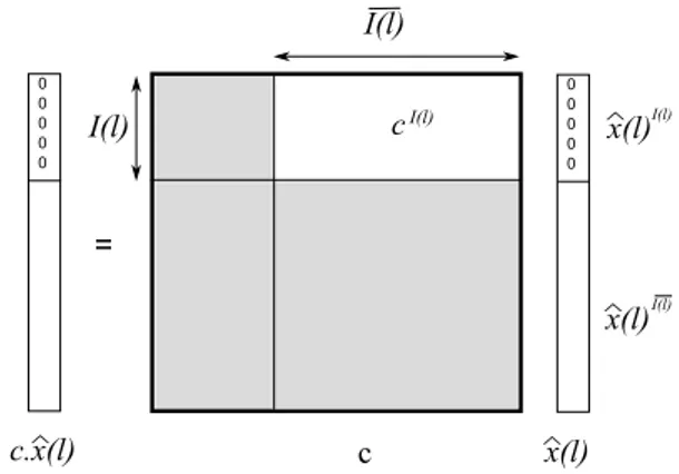
So, if l ∈ Z, let us define I(l) as:
I(l) = {k ∈ {1, . . . , K}, nk 6 | l}
For any integer l, if k ∈ I(l) and i ∈ Ik, then bxi(l) =
c.bxi(l) = 0, so that (with similar convergence arguments
that in the proof of lemma 3.1):
c.bxi(l) = k X j=1 cijxbj(l) 0 = k X j∈I(l) cijbxj(l) + k X j /∈I(l) cijxbj(l) 0 = k X j /∈I(l) cijbxj(l)
Let us write cI(l) the matrix which all coefficients are
zero, except for those of index (i, j) ∈ I(l) × {I(l) which are identical to those of c, and bx(l){I(l) the vector with zero components on the indexes belonging to I(l) and those of bx(l) in for indexes belonging to {I(l).
The previous property can be written (see figure 2):
∀l ∈ Z cI(l)x(l)b {I(l)= 0
This property holds for any integer l, and is empty when l is a multiple of all the ni. So that, if I(l) is the
partition of I defined as:
I(l) =©I(l), {I(l)ª
we can re-write it as:
∀l ∈ Z cI(l)bx(l) = 0
Let us now consider I16= I2(this is possible as K > 1). As those two classes are distinct, there exists l such that
Figure 2: Constraints on the Fourier’s coefficients ˆx(l).
n1does not divide l and n2divides l. As c is regular, cI(l) is thereby injective. We deduce that:
b
x(l){I(l)= 0
This proves that for any l divisible by n2 and not by n1, b
x(l){I(l) is zero. Thus, for any coefficient of bx(l){I(l) to be non zero, n1 must divide l, and consequently (as none of the xi is a constant map) for all i ∈ I2, xi(t) is n1τ0 periodic. This is incompatible with the partition of I. Thus, K = 1 and thereby τ is a constant map (in other words, I is synchronized).
4.5
Perspectives of applications to
classi-cal differential systems
In this last section, we show how the cellular systems point of view may be applied to classic differential systems and how dealing with different Banach spaces
Ei may be useful. This discussion will be enlightened
with a really simple example (finite population).
Let E be a Banach space and F a vector field on E. We want to see how this differential equation may be seen as a cellular system. For instance, one could consider a simple conservative system on E = R4with an Hamilton’s equation given by (see [1])
x0 1 = y1 y0 1 = αx1− βx31+ εx2 x0 2 = y2 y0 2 = −γx2+ εx1
The first step is to identify the different cells of I. We must factorize each term in the equations according to the different variables. For example, the second equation may be seen as:
y01= (α − βx21)x1+ εx2 So that the term (α − βx2
1) has to be a part of the coupler we are building. Moreover, since it is the equation giving
y0
1, and as the way a cell computes how it interprets the
population’s state depends only on its own state, x1 and
y1have to belong to the same cell. In this simple example it is the only case where two variables have to be gathered in the same cell. To end with, this leads to the following structure of cellular system:
I = {1, 2, 3}
with the Banach spaces:
E1= R2, E2= E3= R
As it should often be the case, the associated vector fields are just identity maps on Ei, and the coupler is then:
c = cc1121 cc1222 cc1323 c31 c32 c33 with c11: E1 −→ L(E1) (x1, y1) 7−→ · 0 1 α − βx2 1 0 ¸ c12: E1 −→ L(E2, E1) x2 7−→ · 0 ε ¸ c13: E1 −→ L(E3, E1) y2 7−→ · 0 0 ¸ c21: E2 −→ L(E1, E2) (x1, y1) 7−→ £ 0 0 ¤ c22: E2 −→ L(E2) x2 7−→ £ 0 ¤ c23: E2 −→ L(E3, E2) y2 7−→ £ 1 ¤ c31: E3 −→ L(E1, E3) (x1, y1) 7−→ £ ε 0 ¤ c32: E3 −→ L(E2, E3) x2 7−→ £ −γ ¤ c33: E3 −→ L(E3) y2 7−→ £ 0 ¤
Now, before applying some of the previous techniques, we may compute the different decompositions of c upon different non trivial partitions of I. Those partitions are:
P1= © {1}, {2}, {3ª}, P2= © {1, 2}, {3}ª P3= © {1, 3}, {2}ª, P4= © {1}, {2, 3}ª which gives: c/P1= c021 c012 cc1323 c31 c32 0 c/P2= 00 00 cc1323 c31 c32 0
c/P3= c021 c120 c023 0 c32 0 c/P4= c021 c012 c130 c31 0 0
Now, in order to simplify, we replace the cij that are
identically zero by 0, we obtain the following different matrices: c/P1= 00 c120 c023 c31 c32 0 c/P2= 00 00 c023 c31 c32 0 c/P3= 0 c120 0 c023 0 c32 0 c/P4= 00 c012 00 c31 0 0
In the end, writing the coupler as an application from S to L(S), one finds those four matrices:
0 0 0 0 0 0 ε 0 0 0 0 1 ε 0 −γ 0 0 0 0 0 0 0 0 0 0 0 0 1 ε 0 −γ 0 0 0 0 0 0 0 ε 0 0 0 0 1 0 0 −γ 0 0 0 0 0 0 0 ε 0 0 0 0 0 ε 0 0 0
At this point, we just have to check that the coupler is weakly injective:
ker (c/P1) ∩ E2= ker (c/P4) ∩ E2= {0} ker (c/P2) ∩ E3= ker (c/P3) ∩ E3= {0}
So, we can apply the proposition 4.1 and without any analytic calculus, state that this differential system may not admit any component quasi-periodic solution. In other words, if there exists a component periodic trajectories (which is well known to be true) they must be synchronized.
Moreover, these conclusions may hold in a more gen-eral case were the cij are less simple, and we can easily
produce a result without any effort:
Proposition 4.9 (Generalized coupled pendulum). Let
us consider a differential system which is driven by the following equations:
x0
1 = a1(x1, y1)x1+ a2(x1, y1)y1+ a3(x1, y1)x2 +a4(x1, y1)y2
y0
1 = a5(x1, y1)x1+ a6(x1, y1)y1
x0
2 = a7(x2)x2+ u(x2)y2
y0
2 = ε(y2)x1+ a8(y2)y1− γ(y2)x2+ a9(y2)y2
If the maps u and ε never vanish, then the systems has no component quasi-periodic solution.
This result does not have to be deep in itself, neither has it to be the most general one we could have deduced from the previous discussion. It is just a sketch of how one can handle some structure properties of a differential system, applying lemma 3.1, without going into deep and specific calculus.
On the other hand, we must stress the point that this technique does not solve completely the problem of the existence of quasi-periodic solutions, as one must check by other techniques that there is no quasi-periodic solution which is not component periodic.
5
Conclusion
In this work we have built a general framework of cellu-lar systems in order to handle a wide variety of coupled systems, and therefore a wide class of complex systems. We focused on an emergent property of those dynami-cal systems: the frequencies locking phenomenon. Usu-ally one observes solutions of particular coupled systems and shows that within suitable conditions synchronization must occur. These results are qualitatively dependent on the systems of interest and do not stand in the general cases. We tried to change our point of view and bring out completing results. As we choose not to address the problem of convergence to a periodic solution, we do not prove that synchronization ultimately happens. Instead, we consider the problem at its end: if one supposes that some coupled systems converge to oscillating behaviors, then they must be synchronized, regardless to the indi-vidual dynamical systems (as soon as the maps which define each of them are injective nearby the trajectories). In most papers (see for instance [13]) the population of coupled systems is implicitly defined and has only two cells, sometimes a finite number N , and more rarely an infinity. Moreover, on the contrary of what most stud-ies about synchronization issues state, we do not assume anything concerning the cells dynamics. Especially, we do not assume that they are oscillators. We only assume that they (asymptotically) exhibit periodic behaviors un-der the coupling effects (the first assumption implies the second, but the opposite is clearly false).
We believe that this way of reaching general results about cellular systems gives some explanations about why the frequencies locking phenomenon emerges naturally in a large variety of coupled dynamical systems. Our results show that the following alternative is natural in many cases: either the whole population is synchronized, either its cells cannot all have periodic behaviors.
Another interesting perspective is to apply this strat-egy to differential systems, as we outlined at the end of the fourth section. For example, on the contrary of what happens in general case of hamiltonian systems, where limit torus are generally filled with quasi-periodic trajec-tories (especially after perturbations), our results suggest
that concerning cellular systems, limit torus are mainly filled with periodic trajectories.
Moreover, we have achieved some similar work on a natural generalization of this strategy to non countable population, since, in order to model natural systems, it is often useful to handle continuous populations). We truly think that all those results are only a part of what can be done using cellular systems and that this work enlarges the possibilities of studying synchronization issues in some biologically inspired systems. But the scope of this kind of cellular systems may be beyond synchronization questions, as it is quite general and allows theoretical studies. It could be a promising theoretical tool to model complex systems.
References
[1] A. C. J. Luo, Predictions of quasi-periodic and chaotic motions in nonlinear Hamiltonian systems, Chaos, Solitons & Fractals 28 (3) (2006) 627–649.
[2] M. Bennett, M. F. Schatz, H. Rockwood, K. Wiesenfeld, Huy-gens’s clocks, Proc. R. Soc. Lond. 458 (2002) 563–579. [3] J. Buck, Synchronous rhythmic flashing of fireflies. ii, Quarterly
Review of Biology 63 (3) (1988) 265–289.
[4] L. Bunimovich, Dynamical Systems, Ergodic Theory and Ap-plications, Encyclopaedia of Mathematical Sciences, 2nd ed., Springer, 2000.
[5] G. B. Ermentrout, W. C. Troy, Phaselocking in a reaction-diffusion system with a linear frequency gradient., SIAM-J.-Appl.-Math. 46 (3) (1986) 359–367.
[6] L. Gaubert, Auto-organisation et ´emergence dans les syst`emes coupl´es, individuation de donn´ees issues de syst`emes biologiques coupl´es., Ph.D. thesis, Universit´e de Bretagne Occidentale (2007).
[7] J.-P. Goedgebuer, P. Levy, L. Larger, Laser cryptography by optical chaos, in: J.-P. Goedgebuer, N. Rozanov, S. T. andA.S. Akhmanov, V. Panchenko (eds.), Optical Information, Data Processing and Storage, and Laser Communication Technolo-gies, vol. 5135, 2003.
[8] P. Goel, B. Ermentrout, Synchrony, stability, and firing patterns in pulse-coupled oscillators, PHYSICA D 163 (3-4) (2002) 191– 216.
[9] D. Gonze, J. Halloy, A. Goldbeter, Stochastic models for cicar-dian oscillations: Emergence of a biological rythm, International Journal of Quantum Chemistry 98 (2004) 228–238.
[10] F. C. Hoppensteadt, J. B. Keller, Synchronization of periodical cicada emergences, Science 194 (4262) (1976) 335–337. [11] C. Huygens, Christiani Hugenii Zulichemii, Const. F.
Horologium oscillatorium sive De motu pendulorum ad horolo-gia aptato demonstrationes geometricae, Parisiis : Apud F. Muguet, Paris, France, 1673.
[12] E. M. Izhikevich, F. C. Hoppensteadt, Slowly coupled oscil-lators: Phase dynamics and synchronization, SIAM J. APPL. MATH. 63 (6) (2003) 1935–1953.
[13] N. Kopell, G. B. Ermentrout, Handbook of Dynamical Systems II: Toward Applications, chap. Mechanisms of phase-locking and frequency control in pairs of coupled neural oscillators, Elsevier, Amsterdam, 2002, pp. 3–54.
[14] Y. Kuramoto, Self-entrainment of a population of coupled non-linear oscillators, in: International Symposium on Mathemati-cal Problems in TheoretiMathemati-cal Physics, vol. 39, Springer Berlin / Heidelberg, 1975, pp. 420–422.
[15] Y. Kuramoto, Chemical oscillations, waves, and turbulence, Springer-Verlag, New York, 1984.
[16] S. C. Manrubia, A. S. Mikhailov, D. H. Zanette, Emergence of Dynamical Order. Synchronization Phenomena in Complex Systems, World Scientific, Singapore, 2004.
[17] D. C. Michaels, E. P. Matyas, J. Jalife, Mechanisms of sinoa-trial pacemaker synchronization: A new hypothesis, Circ. Res. 61 (1987) 704–714.
[18] L. M. Pecora, T. L. Carroll, G. A. Johnson, D. J. Mar, J. F. Heagy, Fundamentals of synchronization in chaotic systems, concepts, and applications, Chaos 7 (4) (1997) 520–543. [19] A. Pikovsky, M. Rosenblumand, J. Kurths, Synchronization: A
Universal Concept in Nonlinear Sciences, Cambridge University Press, 2001.
[20] I. Prigogine, Introduction to Thermodynamics of Irreversible Processes, Wiley, New York, 1967.
[21] I. Prigogine, Theoretical Physics and Biology, M Marois, North-Holland: Amesterdam, 1969.
[22] L. Ren, B. G. Ermentrout, Phase locking in chains of multiple-coupled oscillators, PHYSICA D 143 (1-4) (2000) 56–73. [23] Y. G. Sinai, Introduction to ergodic theory, Princeton
Univer-sity Press, 1976.
[24] I. Stewart, M. Golubitsky, Patterns of oscillation in coupled cell systems, in: P. P.Holmes, A.Weinstein (eds.), Geometry, Dynamics and Mechanics: 60th Birthday Volume for J.E. Mars-den, Springer-Verlag, New York, 2002, pp. 243–286.
[25] S. Strogatz, Sync: The Emergeing Science of Spontaneous Or-der, New York: Hyperion, 2003.
[26] A. Winfree, Biological rhythms and the behavior of popula-tions of coupled oscillators, Journal of Theoretical Biology 16 (1) (1967) 15–42.
[27] A. Winfree, The geometry of biological time, Springer- Verlag, New York, 1990.
[28] C. Wu, L. O. Chua, A unified framework for synchroniza-tion and control of dynamical systems, Tech. Rep. UCB/ERL M94/28, EECS Department, University of California, Berkeley (1994).