HAL Id: hal-02393135
https://hal-mines-paristech.archives-ouvertes.fr/hal-02393135
Submitted on 4 Dec 2019
HAL is a multi-disciplinary open access
archive for the deposit and dissemination of
sci-entific research documents, whether they are
pub-lished or not. The documents may come from
teaching and research institutions in France or
abroad, or from public or private research centers.
L’archive ouverte pluridisciplinaire HAL, est
destinée au dépôt et à la diffusion de documents
scientifiques de niveau recherche, publiés ou non,
émanant des établissements d’enseignement et de
recherche français ou étrangers, des laboratoires
publics ou privés.
SCALE
Thomas Berthou, Bruno Duplessis, Philippe Rivière, Pascal Stabat, Damien
Casetta, Dominique Marchio
To cite this version:
Thomas Berthou, Bruno Duplessis, Philippe Rivière, Pascal Stabat, Damien Casetta, et al..
SMART-E: A TOOL FOR ENERGY DEMAND SIMULATION AND OPTIMIZATION AT THE CITY
SCALE. BS2015, Aug 2015, Chambéry, France. �hal-02393135�
SMART-E: A TOOL FOR ENERGY DEMAND SIMULATION AND
OPTIMIZATION AT THE CITY SCALE
Thomas Berthou, Bruno Duplessis, Philippe Rivière, Pascal Stabat, Damien Casetta,
Dominique Marchio
Mines ParisTech, PSL Research University, Centre for energy efficiency of systems
ABSTRACT
Adding flexibility to the demand may rationalize energy production. Indeed, it should be possible to maximize the use of low CO2 and low-cost energy
production systems by managing the demand at the city scale. In this context, numerical simulation may be a great help for setting up various demand response (DR) strategies in a short-term. For that purpose, a simulation environment called Smart-E which focuses on the thermal and electrical uses of energy in dwellings and commercial buildings has been developed. This library of algorithms is specially designed to simulate hypothetical or real cities and it uses techno-explicit bottom-up models fed with public databases and the specific users’ data. First the paper presents the Smart-E tool architecture. Then, a case study is conducted on a French typical medium city to show how Smart-E may help the aggregator to predict the impact of specific DR strategies. For this purpose two load shedding strategies are tested at the city scale with indoor temperature comfort criteria. Strategies reduce maximum electric power for heating by 25% for 24h.
INTRODUCTION
Since the building sector is responsible for 40 % of the total European energy consumption (IEA, 2014) managing the energy consumption in buildings at the city scale may help to rationalize the energy production and to optimize the electricity grid. Indeed, intermittent renewable energies should represent 17% to 20% of the total electricity production in Europe by 2020 (EREC, 2010). To guarantee the electric grid balance and limit the use of peaking power plants, the intermittent energy plants should be complemented with demand response (DR) strategies and the use of smart appliances in a smart grid territory. The objective is to propose an energy simulation tool at the city scale with realistic bottom-up systems’ models adapted to intensive calculation and the diversity of information on buildings. Simulating the energy demand of building stocks should help energy actors in several ways:
- Help standards design and investment decisions by simulating and comparing the possible scenarios in a specific territory (e.g. stimulus to renovation, standards for new buildings).
- Anticipate the energy network long-term evolution by simulating new uses of energy (e.g. electric cars) - Help the short-term networks balance by proposing demand response strategies and avoiding the discomfort created by network failure and limiting the use of polluting peak load production.
- Optimize smart grids in real-time by sending the best orders to the connected appliances (consumption at best time).
Eventually, the Smart-E tool is designed to answer these four issues, but this paper only focuses on realistic demand response strategies implemented on residential buildings in a smart grid context to help short-term grid balance.
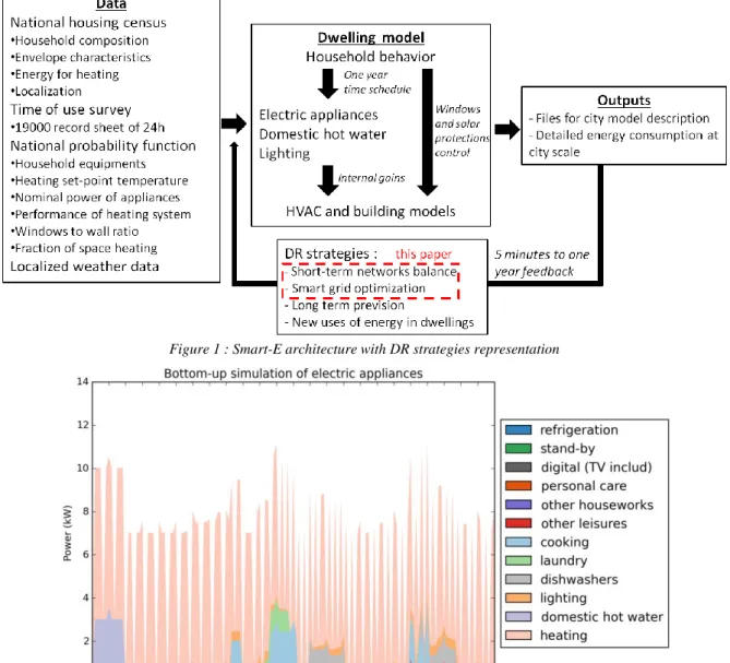
After a short review this paper presents the databases used for simulation, then the bottom-up models used in Smart-E. Finally a case study on short time DR strategies is conducted on an existing medium sized French city. The strategies control the set-points of heating electricity systems at the city scale to meet the need in terms of aggregated power reduction during 24 hours. Figure 1 shows the Smart-E architecture and introduces the following sections.
State of the art on bottom up energy city modeling
The bottom-up approach is described as “built up from data” (Kavgic, et al., 2010). Indeed a strong connection between the degree of model details, the data availability and the scale of simulation (i.e. street, district, city or territory) is observed. We aim to simulate hundreds of buildings simultaneously at the city or territory scale. At this scale of simulation, an existing building database is needed and it is not realistic to fill in specific information on the building such as shape, orientation, household information manually. Therefore the physical and stochastic models must be adapted to the diversity of building information and design to reduce uncertainties. Tools for energy simulation in cities exist but are not totally adapted to our needs or not publicly available. Two families of tools can be distinguished: detailed models which are constrained by data availability and
are more adapted to the street or district simulation scale. Then, the simplified physical and stochastic models which need less detailed data but are only accurate on an aggregated level.
UMI (Reinhart, et al., 2013) and CitySim (Robinson, et al., 2009) are detailed multi-energy modeling environments, with 3D representation of buildings. Since these tools are easily connected to existing geometrical information databases like BIM (Building Information Modeling) standard or OpenStreetMaps they can access detailed building shapes and orientations. Despite this, they are more adapted for medium scale simulation (street or district) in which all the building thermal characteristics and HVAC systems’ information can be manually documented. Fonseca and Schlueter (2015) connect both approaches and propose a 4D representation of a city district with bottom-up energy models. It might be the most advanced tool for city simulation however remains very dependent on data availability. SynPRO (Ficher, et al., 2015) and the tool of Richardson et al. (2010) focus on the electricity consumption of dwellings and have been validated with a complete monitoring program. The needed data are mostly stochastic so the platform is well adapted to city scale simulation. EnergGis (Girardin, et al., 2010), SYNCITY (Keirstead, et al., 2009) and Artelys Crystal City (Page, et al., 2013) are designed to plan energy infrastructure (networks and power plants) in new territories. The energy demand information does not originate from bottom-up models of specific uses. Good et al. (2015) and Shimoda et al. (2004) propose energy models for domestic demand profiles and use stochastic and simple physical models to simulate electricity, gas and heat consumption. These tools are especially adapted to short time DR strategies for network balance and smart grid optimization and have many similarities with Smart-E. Table 1 summarizes information about bottom-up city energy simulation tools.
DATABASE PRESENTATION
Time of use survey (ToU)
French ToU survey is used to simulate occupants’ activities (INSEE, 2009). The database is composed of 19000 record sheets of 24 hours with more than 100 possible activities which last 10 minutes at least. Wilke et al. (2013) create a global probabilistic model of household activities with the same survey conducted 10 years earlier from which household electric power profiles are deduced. In this paper a similar but simpler approach is used. Instead of using a specific model, one week time table from the concatenation of 24 hours record sheets is built for each occupant. Working days and weekends are respected; workers, pensioners and students are set apart from other individuals. At an aggregated level the results are very similar to Wilke’s probabilistic
model. The survey activities are sorted out in 9 classes presented in the “Model description” section.
Table 1
Urban energy simulation tools comparison
Name Main objective Scale of simulation
UMI Highly detailed building energy simulation
Street to district CitySim Urban planning Street to
district Fonseca et al Education and urban
planning
Street to district SynPRO Residential electricity
simulation City to territory Richardson et al. Residential electricity simulation City to territory EnerGis Energy system
integration Territory Syncity Energy Network
integration Territory Artelys
Crystal City Infrastructure planning Territory Good et al. Detailed energy demand
simulation
City to territory Shimoda et al. Stochastic residential
electricity simulation City to territory Smart-E Implementation of DR strategies in Cities City to territory
National housing census
The French national census on housing and household description is used for dwelling description (INSEE, 2011). The census information and the interaction with models’ parameters are described in table 2. Information is available for 100% of dwellings in small cities (less than 10k inhabitants) and only 40% for medium and large cities (more than 10k inhabitants).
Table 2
National census information used by Smart-E
Census information Models Used
Dwelling construction year
Envelope performance, retrofit probability
Dwelling area Inertia, heated area Energy for heating Type of HVAC system Household composition
(age, activities)
Appliances used, hot water system, internal heat gain Number of occurrence in
city Weight of dwelling in city Single or multi-housing Heat loss surface
Localization Weather data
Data availability issues
Smart-E is designed to simulate any city, yet available data vary a lot from a city to another. A specific method is used for the data availability problem. Several levels of data information are used, from very detailed to aggregated information. High detailed information at the building level is used in priority. When they are not available in the studied territory, probabilistic functions or even average or median values are used. Table 3 describes the four levels of information existing in Smart-E. In the case
study, data from level 1 to 4 are used. During the models’ adjustment process, levels of information 1 and 2 are optimized using a heuristic method (see model adjustment section).
Table 3
City database level information
Level Description Generation of diversity
Example from the case
study
1 Median or
average value Low
Installed lighting power 2 Probabilistic function at territory scale Medium Efficiency of appliances 3 Probabilistic function at city scale
High Retirees ratio
4
Information known for each
housing Very high Floor area, Energy for heating
MODELS DESCRIPTION
In this section, each model is described and some arguments are given to show how they meet the needs in terms of data availability and computing time. In Smart-E, the models’ complexity is driven by DR strategies design and not by uncertainties reduction concerns. Indeed a sensibility analysis for energy in city simulation shows three parameters which highly impact city energy consumption (Booth, et al., 2012):
- Fraction of space heated
- Internal heating set-point temperature - Coefficient of performance for the heating
system
Since these parameters are coming from stochastic models where the values are highly uncertain it seems worthless to use detailed envelope or system models for city simulation to reduce energy calculation uncertainties. Therefore the complexity of the models should be adapted to DR strategies design, for example a multi-zone dwelling model should be used only if the simulated DR strategy optimizes distinctly each zone. In this paper the DR strategy aims to optimize systems by modifying the indoor temperature set-point. A specific model for systems’ control should thus be used.
Heating systems and envelope models
A second order differential equation is used for the envelope modeling. This mono-zone model has been validated for electric consumption and indoor temperature prediction in tertiary buildings (Berthou, et al., 2013), (Berthou, et al., 2014). With only 10 parameters the model is configurable from easy to find information on dwellings (e.g. floor area, built year) and could be optimized to reach a specific consumption value. The window’s opening can be simulated by changing a specific parameter value and the solar protection closing effect by reducing the solar flux power on the windows.
Solar radiations on buildings are calculated from the Meteonorm database. Dwellings are simulated as north-south oriented. For gas, domestic fuel and electric heating systems, constant efficiency ratios are used. For thermodynamic systems, a linear correlation with outdoor temperature is used. Heating systems are sized with a realistic static method used by installers. A proportional gain is used for heating systems control model with a 0.5 °C dead band.
Domestic hot water (DHW)
ToU data are used to simulate hot water consumption associated with activities presented in table 5. A hot water volume associated with an electric water heating system is simulated as a homogeneous water volume at 60°C depending on the area of dwellings. Electric DHW systems can receive orders from the grid to force heating start-up depending on the city localization. In this paper we assume that 75% of the storage electric water heaters are controlled between 10 a.m. and midnight and the other 25% can start at any time during the day when the internal tank temperature becomes too low. Non electric DHW systems are considered as instantaneous hot water production systems and are directly linked to hot water use.
Lighting
Lighting consumption is based on an in-situ campaign (Alessandrini, et al., 2006) and is calculated from the French standard model (CSTB, 2010). The first step is to calculate the dwelling indoor illumination from weather and geometrical information then a piecewise linear function gives the light surface ratio from the illumination value. Table 4 shows examples of function outputs. It is assumed that all the lights are turned-off when the dwelling is empty or when everyone is asleep. The surface power probability of light is calculated from the adjustment process.
Table 4
Inflexion points of light function calculation Light surface ratio Indoor illumination (lux)
100% < 100
30% 700
0% >2800
Other electric and gas appliances
ToU data are used to describe occupants’ activities and generate weekly time tables. Each occupant who might have an interaction with the energy consumption in the dwelling is simulated during one week (i.e. occupant older than 11). Then the same week is repeated all the year (a weekly organization of the households is assumed). Occupants have 9 possible activities (table 5) and can do up to 2 activities at a time with exceptions (no possibility to sleep and eat for instance). For each activity and each household an electrical power is calculated from a statistical distribution. The powers of systems are taken from the Enertech database (Enertech, 2010).
Figure 1 : Smart-E architecture with DR strategies representation
Figure 2: One day electric consumption of a single housing during winter (140 m², 4 occupants), 10 min time step simulation
Figure 3: One day electric consumption for 12 000 dwellings during winter in Palaiseau, only 19% of dwellings use electric heating systems, 10 min simulation time step
We assume people from a same household don’t have any interaction with each other but if two occupants from a same household accomplish the same activity at the same time the power consumption associated with this particular activity remains the same.
“Wash the dishes” and “laundry” activities are differentiated from the others because occupants can do other activities when those are not handmade. The refrigeration electric consumption is calculated with a stochastic model from the Enertech database. No interaction between refrigeration systems and occupants or other exogenous parameters are simulated for instance. Stand-by consumption for electric appliances is added to each dwelling and is picked from a probabilistic function.
Figure 2 presents the electric consumption of a medium size dwelling during a working day in winter simulated with Smart-E. This house is equipped with electric convectors and a storage electric water heater. These results come from a poorly insulated single-house which explains the high electric consumption for heating. This figure illustrates how Smart-E overlaps consumption from different types of models (simple physic model and stochastic model) to reconstruct global electric load of a specific dwelling. Each dwelling load is different and recreates a realistic diversity of consumption profiles. Figure 3 presents the aggregated electric consumption of dwellings for a medium French city. This shows the weight of each energy usage in the total infra-day electric consumption during winter. This figure helps to realize a visual validation of Smart-E aggregated power:
- Day and night distinction for human activity consumption types
- 3 peaks for cooking activities: breakfast, lunch and diner
- Use of dishwasher after meal time
- High use ratio of digital appliances during lunch time and during the evening
- High consumption for DHW during the night (French specificities)
- High consumption for heating during cold days Table 5
Merge activities of the ToU survey
Activity Name details Type of consumption Digital TV, computer, video game, DVD player, phone Electricity Cooking Cooking plate, microwave, oven, cook top
Hot water, gas and electricity consumption Meal Action of eating None
Rest Nap and sleep Lighting turn off Personal car Bath, shower, body
care, Hot water consumption Other leisure Game, homework, reading…, None Other
housework Hoover, iron Electricity Wash the
dishes
Hand washing or dishwasher
Hot water and electricity Laundry
Hand washing or with a washing machine and dryer
Hot water and electricity
Model adjustment and aggregation
The total annual consumptions database of each energy usage serves for smart-E validation (CEREN, 2013), (Almeida, et al., 2011). The power probability density function associated to each type of appliance is adjusted with a heuristic method to match the annual energy objective. For example the refrigeration appliances should represent 28% of dwelling electric consumption excluding electric space and water heating. After optimization, a probability function for power refrigeration systems is proposed (table 6). The ToU model is considered to be sufficiently detailed and validated so we decided not to optimize it during the adjustment process.
As a result, the simulations are validated at an aggregated level and in annual energy consumption only. Compared to the measured consumption at the dwelling level an important bias can be observed (Ficher, et al., 2015). Grandjean (2013) suggests that aggregation phenomena in simulated domestic appliances converged from 1000 individuals. Accordingly special attention will be paid to use Smart-E with over 1000 dwellings simulation problems. Limitations in Smart-E validation process must be considered in DR strategies design by proposing aggregated optimization problems only.
Table 6
Power distribution of the refrigeration systems Power (W) Probability (%) 0 (no refrigeration) 1.0 240 20.3 300 20.7 480 14.5 540 29.5 600 14.0
CASE STUDY
Balance problems between electricity production and demand might happen during cold periods in France (RTE, 2012). Indeed a cold period can create high electricity consumption for heating associated with low wind plants production and low solar plants production. If no substitute power plants are available or remain too polluting and expensive, a need for 24 hours DR strategies on electricity demand at the city scale can occur. Since heating represents a large part of the electricity consumption during cold periods and can be easily controllable, the proposed strategies modify the electric heating systems’ set-points. Furthermore the inertia phenomenon reduces discomfort effects on
household by limiting the indoor temperature speed variation.
For the need of the study all the electric heating systems are assumed to be operated by an aggregator: - Heating Systems can receive instantaneous indoor temperature set-point orders from the aggregator. - An order not compatible with the comfort condition can be rejected by the system, in such cases the set-point remains constant. In the case study the order is rejected when the indoor temperature is below 18°C. - The aggregator can’t know in advance the energy state of the dwellings; that is why the DR strategies must be simulated before being carried out for real.
Presentation of the case study
The DR strategies are conducted on a common medium size French city named Palaiseau which is composed of 12 241 dwellings among which 19.4% use an electric system for heating. This represents more than 50% of the total electric power during cold periods. Table 7 gives general information about dwellings in Palaiseau.
Table 7
Summary of the case study Inhabitants 29281 Average Elevation 100 m Climate Oceanic Dwellings 12241 Median floor area 59 m² Investigated dwellings in
census 40%
Single dwelling 38% Energy for heating
City gas: 58% Electricity: 19% District heating: 5% Other (fuel, wood, …): 18%
Design of two DR strategies
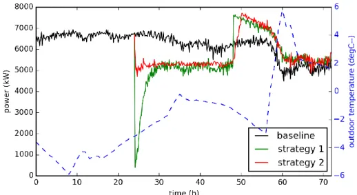
Two DR strategies are compared in this paper using simulation during a cold day with Palaiseau data. The first strategy (strategy 1) sends the same indoor temperature set-point (18°C) to all the electric heating systems during 24 hours. No objective on the total electric consumption is set. For the second strategy (strategy 2) we aim to reduce the maximal electric power for heating by 25% which represent a 1.7 MW load shedding at the peak time. To reach this objective, every 10 minutes 20% of dwellings selected randomly receive an optimized indoor temperature set-point which is maintained during two hours. A same dwelling set-point can be optimized several times in two hours.
Results and discussion
Both strategies are simulated with Smart-E on the same winter day. Figure 4 shows 3 days of the total heating electric consumption. The DR strategies take place during the second day and the baseline is a simulation without DR strategies.
Results of strategy 1 can be decomposed into 3 steps:
Step 1 (0 p.m. to 6 p.m.): All the heating systems stop at 0 p.m. when they receive the new set-point except the one with an indoor temperature below 18°C (figure 5). After the indoor temperature reaches the new set-point, the heating systems restart. The restart time depends mostly on the envelope’s characteristics.
Step 2 (6 p.m. to 24 a.m.): The new set-point reduces the power by almost 25%. Even if the power seems to be constant, the outdoor temperature and other exogenous phenomena still have an impact.
Step 3 (after 24 a.m.): All dwellings resume their former set-point values which increase the power in a very short time. Due to dwelling inertia, the consumption of strategy 1 is above the baseline for almost a day to compensate the load shedding. Strategy 1 succeeds to reduce the total heating power by 25% from the maximum baseline. But short time power variation at the beginning and the end of the strategy can be damaging for grid balance. The indoor temperatures are constant for all dwellings during all the day which limits the discomfort. Results of strategy 2 can be decomposed into 2 steps: Step 1 (0 p.m. to 24 a.m.): Every 10 minutes the strategy optimizes the set-point order of 20% of dwellings to reach the objective of aggregated power value (figure 6). The objective is not reached at each step but the consumption is nearly constant and the power variations are smoother during the first hours. Furthermore, the orders are corrected from the exogenous phenomena thanks to the optimization process. A set-point of a same dwelling can change several times during 24 hours.
Step 2 (after 24 a.m.): The dwellings resume their old set point values randomly staggered over two hours (figure 5). As a result the power rise is smoother than for strategy 1. Once again the consumption after the DR strategy is above the baseline due to inertia effects.
Strategy 2 succeeds to reduce the total heating power by 25% from the maximum baseline and proposes controlled short time power variation which is more acceptable for the grid. On the other hand the indoor temperature may change several times in 24h for a same dwelling which can be less comfortable for occupants.
From an energy point of view both DR strategies do not have a notable impact due to energy recovery phenomena.
CONCLUSION
The paper describes a new tool named Smart-E which aims to simulate the energy demand at the city scale. After a description of its architecture, Smart-E is used to compare two DR strategies on their impact on the comfort and the aggregated electric load curve. Both strategies reduce the maximum total electric power by 25%.
Figure 4: Impact of DR strategies on total electric consumption of heating systems (3 days), outdoor temperature (--)
Figure 5: Impact of the first DR strategy on indoor temperature (top) and set point (bottom), average curve of all dwellings (black), examples of specific dwellings curves (not-black)
Figure 6: Impact of the second DR strategy on indoor temperature (top) and set point (bottom), average curve of all dwellings (black), examples of specific dwellings curves (not-black)
The first strategy uses all the potential for shaving but creates short time electric demand variation which is damaging for the grid. The second strategy shaves 20% of dwellings for 2 hours every 10 minutes with an optimized set-point. As a result the total electric power is better controlled and smoother. The study shows that Smart-E allows to design and to test various DR strategies at the city scale and could be used to optimize energy networks in a smart grid context.
Further works on Smart-E will contribute to validating the platform at several scales including the intra-day power of each appliance. To meet this need a measurement campaign could be realized by monitoring each appliance of hundreds of dwellings. The next step is to simulate the energy consumption of commercial buildings.
REFERENCES
Alessandrini, J.-M., Fleury, E., Filfli, S. & Marchio, D., 2006. Impact de la gestion de l’éclairage et des protections solaires sur la consommation d’énergie de bâtiments de bureaux climatisés. Climamed.
Almeida, A., Fonseca, P., Schlomann, B. & Feilberg, N., 2011. Characterization of the household electricity consumption in the EU, potential energy savings and specific policy recommendations. Energy and Buildings, Issue 43.
Berthou, T., Stabat, P., Salvazet, R. & Marchio, D., 2013. Optimal control for buidling heating: an elementary school case study. IBPSA.
Berthou, T., Stabat, P., Salvazet, R. & Marchio, D., 2014. Development and validation of a grey box model to predict thermal behavior of occupied office buildings. Energy and Buildings, Issue 74. Booth, A., Choudhary, R. & Spiegelhalter, D. J., 2012. Handling uncertainty in housing stock models. Building and Environment, Issue 48. CEREN, 2013. Données statistiques du CEREN.
http://www.ceren.fr/ [Online].
CSTB, 2010. Réglementation thermique 2012. Centre scientifique et technique du bâtiment. Enertech, 2010. La mesure des consommations
électriques. http://www.enertech.fr/ [Online]. EREC, 2010. Renewable Energy Technology
Roadmap. European Renewable Energy Concil. Ficher, D., Hartl, A. & Wille-Haussmann, B., 2015.
Model for electric load profiles with high time resolution for German households. Energy and Buildings, Issue 92.
Fonseca, J. A. & Schlueter, A., 2015. Integrated model for characterization of spatiotemporal building energy consumption patterns in
neighborhoods and city districts. Applied Energy, Issue 142.
Girardin, L. et al., 2010. EnerGis: A geographical information based system for the evaluation of integrated energy conversion systems in urban areas. Energy, Issue 35.
Good, N., Zhang, L., Navarro-Espinosa, A. & Mancarella, P., 2015. High resolution modelling of multi-energy domestic demand profiles. Applied Energy, Issue 137.
Grandjean, A., 2013. Introduction de non linéarités et de non stationnarités dans les modèles de représentation de la demande électrique résidentielle. Thesis, Mines ParisTech.
INSEE, 2009. Time of use survey. http://www.insee.fr/ [Online].
INSEE, 2011. fichiers détail du recensement de la population 2010. http://www.insee.fr/ [Online]. IEA, International Energy Agency, 2014. Energy
consumtion by sector. http://www.iea.org/ [Online].
Kavgic, M. et al., 2010. A review of bottom-up building stock models for energy consumption in the residential sector. Building and Environment. Issue 45
Keirstead, J., Samsatli, N. & Shah, N., 2009. SYNCITY: an integrated tool kit for urban energy systems modelling. Urban Research Symposium.
Page, J. et al., 2013. A multi-energy modelling, simulation, and optimization environment for urban energy infrastructure planning. IBPSA. Reinhart, C. F. et al., 2013. UMI - An urban
simulation environment for building energy use, daylighting, and walkability. IBPSA
Richardson, I., Thomson, M., Infield, D. & Clifford, C., 2010. Domestic electricity use: A high-resolution energy demand model. Energy and Buildings, Issue 42.
Robinson, D. et al., 2009. CITYSIM: comprehensive micro-simulation of resource flows for sustainable urban planning. Building Simulation. RTE, 2012. Bilan prévisionnel de l'équilibre offre-demande d'électricité en France. http://www.rte-france.com/ [Online].
Shimoda, Y., Takuro, F., Takao, M. & Minoru, M., 2004. Residential end-use energy simulation at city scale. Building and Environment, Issue 39. Wilke, U., Haldi, F., Scartezzini, J.-L. & Robinson,
D., 2013. A bottom-up stochastic model to predict building occupants’ time-dependent activities. Building and Environment, Issue 60.