HAL Id: hal-00649039
https://hal.archives-ouvertes.fr/hal-00649039
Submitted on 7 Dec 2011
HAL is a multi-disciplinary open access
archive for the deposit and dissemination of
sci-entific research documents, whether they are
pub-lished or not. The documents may come from
teaching and research institutions in France or
abroad, or from public or private research centers.
L’archive ouverte pluridisciplinaire HAL, est
destinée au dépôt et à la diffusion de documents
scientifiques de niveau recherche, publiés ou non,
émanant des établissements d’enseignement et de
recherche français ou étrangers, des laboratoires
publics ou privés.
Preemption Delay Analysis for Floating Non-Preemptive
Region Scheduling
José Marinho, Vincent Nélis, Stefan M. Petters, Isabelle Puaut
To cite this version:
José Marinho, Vincent Nélis, Stefan M. Petters, Isabelle Puaut. Preemption Delay Analysis for
Floating Non-Preemptive Region Scheduling. 2011. �hal-00649039�
Preemption Delay Analysis for Floating
Non-Preemptive Region Scheduling
www.hurray.isep.ipp.pt
Technical Report
HURRAY-TR-111202
Version:
Date: 12-05-2011
José Marinho
Vincent Nélis
Stefan M. Petters
Isabelle Puaut
Technical Report HURRAY-TR-111202 Preemption Delay Analysis for Floating Non-Preemptive Region Scheduling
© IPP Hurray! Research Group
www.hurray.isep.ipp.pt 1
Preemption Delay Analysis for Floating Non-Preemptive Region Scheduling
José Marinho, Vincent Nélis, Stefan M. Petters, Isabelle Puaut
IPP-HURRAY!
Polytechnic Institute of Porto (ISEP-IPP) Rua Dr. António Bernardino de Almeida, 431 4200-072 Porto Portugal Tel.: +351.22.8340509, Fax: +351.22.8340509 E-mail: http://www.hurray.isep.ipp.pt
Abstract
In real-time systems, there are two distinct trends for scheduling task sets on unicore systems: non-preemptive and preemptive scheduling. Non-preemptive scheduling is obviously not subject to any preemption delay but its schedulability may be quite poor, whereas fully preemptive scheduling is subject to preemption delay, but benefits from a higher flexibility in the scheduling decisions. The time-delay involved by task preemptions is a major source of pessimism in the analysis of the task Worst-Case Execution Time (WCET) in real-time systems. Preemptive scheduling policies including non-preemptive regions are a hybrid solution between non-preemptive and fully preemptive scheduling paradigms, which enables to conjugate both world's benefits. In this paper, we exploit the connection between the progression of a task in its operations, and the knowledge of the preemption delays as a function of its progression. The pessimism in the preemption delay estimation is then reduced in comparison to state of the art methods, due to the increase in information available in the analysis.
Preemption Delay Analysis for Floating
Non-Preemptive Region Scheduling
Jos´e Manuel Marinho
∗, Vincent N´elis
∗, Stefan M. Petters
∗, Isabelle Puaut
† ∗CISTER-ISEP Research Centre, Polytechnic Institute of Porto, Portugal†University of Rennes 1, UEB, IRISA, Rennes, France
Email: {jmsm,nelis,smp}@isep.ipp.pt , [email protected]
Abstract—In real-time systems, there are two distinct trends for scheduling task sets on unicore systems: non-preemptive and preemp-tive scheduling. Non-preemppreemp-tive scheduling is obviously not subject to any preemption delay but its schedulability may be quite poor, whereas fully preemptive scheduling is subject to preemption delay, but benefits from a higher flexibility in the scheduling decisions. The time-delay involved by task preemptions is a major source of pessimism in the analysis of the task Worst-Case Execution Time (WCET) in real-time systems. Preemptive scheduling policies including non-preemptive regions are a hybrid solution between non-preemptive and fully preemptive scheduling paradigms, which enables to conjugate both world’s benefits. In this paper, we exploit the connection between the progression of a task in its operations, and the knowledge of the preemption delays as a function of its progression. The pessimism in the preemption delay estimation is then reduced in comparison to state of the art methods, due to the increase in information available in the analysis.
I. INTRODUCTION
Nowadays processors are composed of several subsystems (such as caches, pipelines, transfer lookaside buffers, etc.) which display, at any time-instant, an associated “state”. In the context of this work, what we understand by “state of a subsystem” is the history information enclosed in the subsystem, as well as its logical configuration, at a particular time-instant. For example, the state of a cache at a given time-instant can be seen as a snapshot of all the information stored in that cache at that instant. The objective of this state is to accelerate average-case execution times. All these processor subsystems quasi-continuously face state changes at run-time and we are concerned with state changes which affect the temporal behavior of the executing tasks. In particular, it is the case for task preemptions: when a task resumes its execution (after being preempted), for example, the cache(s) will display a state which is different from its state at the time the task got interrupted. If its state has been substantially altered during the time the task was pending, it is likely that it might be needed to reconstruct at least partially its working set after the the task resumes execution.
Reconstructing the subsystems’ states is attached to time penal-ties in real processors, which may increase the execution time of a task by non-negligible amounts of time. In general purpose computing this effect is balanced by the usually huge performance gains by deploying such state carrying sub-systems and hence is in most cases ignored. In embedded real-time systems, where timeliness is an essential property of the system and is hence thoroughly analysed, these penalties need to be carefully evaluated to ensure that all deadlines are met.
In this work we will mainly focus on the cache-related preemp-tion delay (CRPD), because this delay has the most important
impact on the variation of the execution time of a preempted task [1]. Knowledge of preemption delays is crucial for the assessment of the timing behavior of task-sets when scheduled by a given scheduling policy.
Real-time scheduling policies may be broken into three broad categories, with respect to how preemptions are handled: (a) Non-preemptive scheduling, where task preemptions are not allowed, (b) Fully-preemptive scheduling, where the highest priority active task always gets hold of the processor as soon as it arrives in the system (by interrupting the current executing task if needed), and (c) Limited preemptive scheduling, a hybrid solution between non- and fully-preemptive scheduling. This latter category can be itself divided into two subcategories: fixed non-preemptive region scheduling, where preemption points are hard-coded in the task’s code and preemptions are allowed only when the execution of a task reaches one of these preemption points, and floating non-preemptive region scheduling. In the latter one, whenever a higher priority task is released, the currently running task starts to execute in a non-preemptive region. The length of this non-preemptive region is constant and defined in static time for each task. When the duration of the non-preemptive region elapses, the regular priority relationship between tasks is applied and the task with the highest priority is dispatched onto the processor potentially collating several preemptions into a single point.
On the one hand the floating non-preemptive regions model is more flexible than the fixed one and does not require modifications in the applications. On the other hand it restricts the time-locations at which the preemptions may take place, which makes it more predictable than fully-preemptive scheduling policies. These poli-cies thus provide the system designer with more information about how the system will behave and decrease the pessimism involved in the analysis. It is important to state that the schedulability of these restricted preemption policies dominate over the fully preemptive ones [2]. The theory devised onwards assumes the scheduling using floating non-preemptive regions and proposes a new approach to safely but more tightly bound the preemption delay suffered by a task when compared to the state-of-the-art.
II. RELATEDWORK ANDCONTRIBUTION
CRPD estimation has been a subject of wide study. Several methods have been proposed that provide an off-line estimation based on static analysis, for this inter-task interference value. Even though the work was later refined we will only discuss initial work. Lee et al. presented one of the earliest works on CRPD estimation for instruction-caches [3] where the concept of useful cache blocks was introduced.
Computation of the CRPD in data caches has been proposed by Ramaprasad and Mueller [4]. Since the assumption used in [3], that the value of CRPD throughout a control flow graph’s basic block would remain constant, no longer holds for data caches a different approach had to be devised.
Preemption delay estimation is of little value without its integra-tion into the schedulability test of the systems. Since preempintegra-tion delay is affected by all elements of the task-set several approaches exist to handle this situation. Scheduling analysis by Lee [3] is based on response-time analysis (RTA) by using the k highest values of preemption delay and incorporating that quantity into the response time of the task. Lee uses integer linear programming (ILP) to compute the preemption delay suffered by each task.
Busquets et al. also used RTA [5], but considered the maximum effect the preempted task may suffer by multiplying the number of preemptions with the maximum CRPD. While this is more pessimistic than Lee’s approach, it removes the complex analysis of intersecting cache sets which for realistically sized programs suffers from heavy state explosion.
Also a less complex algorithm in comparison to Lee’s resorting to RTA was presented by Petters and F¨arber [1]. Opposed to Busquets’ approach Petters uses the knowledge of the maximum damage each preempting task may cause instead of only con-sidering the worst-case preemption delay. The ILP problem is addressed by using an iterative algorithm.
Altmeyer et al. presents a summary of all of the literature so far relative to preemption delay on fully preemptive fixed task priority [6]. The authors also presented an enhancement to the available work by merging the approaches of Petters and Busquets in a safe way and considering jitter and the preemption delay suffered by the shared resource execution. A demand-bound function based procedure has been proposed by Ju et al. [7], while the general approach of computing the CRPD is similar to Lee’s approach.
All of the presented preemption delay-aware schedulability tests are specific to fully preemptive scheduling and are much more pessimistic than the one presented in this work since they do not consider the evolution of the preemption delay with the program progression of the preempted task. Our approach differs from past work in the sense that it ties the preemption delay with program-execution progression, thus enabling less pessimism in the preemption delay estimation.
Restricting preemption points presents a viable way to address the problem of preemption delay. The mechanism of preemption deferral was first proposed by Burns et al. [8]. It has a number of advantages as has been pointed out in several works e.g. [9], [10]. In particular, Gang Yao et al. provide a comparison of all the available methods described so far in literature [10] regarding restricted preemptive scheduling using fixed task priority.
Bertogna and Baruah have devised a method to compute the size of the non-preemptive regions, for earliest deadline first (EDF) scheduling policy, using a demand-bound function based technique [2]. In this work the slack in the schedule depending on the length of the interval, assuming synchronous release of all the tasks, is computed. The method fits both the fixed non-preemptive region model and the floating one.
Several methods addressing the same issue in fixed task priority exist [11], [12]. A fixed priority scheduling method has been
devised by Gang Yao et al. [11], where a maximum bound on the length of fixed non-preemptive regions is provided. In this situation the computed length of the fixed non-preemptive regions are generally larger than in previous work, as the last chunk of a task’s execution is not subject to further preemptions. This enables a further reduction on the number of preemptions.
Marinho and Petters presented a method to increase, at run-time, the length of the preemption triggered floating non-preemptive regions for fixed task priority [12]. This method is taking advantage of off-line knowledge and on-line task release information to increase the length of the non-preemptive regions. This leads generally to a steep decrease on the preemptions suf-fered. Similar to previous work the preemption delay problem was not addressed in their work. Reducing the number of preemptions helps decreasing the pessimism added to the schedulability test.
The preemption delay estimation problem using fixed non-preemptive region scheduling was presented by Bertogna et al. [13]. In order to reduce CRPD, the usage of fixed non-preemptive areas of code is proposed. The preemption points are thus re-duced to a small number of well defined points. In this way the maximum CRPD is decreased and overall system’s response time is enhanced. This work has the limitation that it requires manipulation of the code of tasks and thus is not very amenable to system developers. In particular, it is not straightforward to take into account tasks with complex control flow graphs [13]. Additionally it can not be easily applied in situations where the task-sets are subject to run-time change, since the maximum allowed distance between preemption points is defined by the higher priority workload.
Our work addresses the computation of the preemption delay in systems using preemption triggered floating non-preemptive regions which was previously not covered in the literature.
III. SYSTEMMODEL
The system consists of a task set τ = {τ1, . . . , τn} scheduled
to run on a single core processor. Each task τi may generate a
potentially infinite sequence of jobs, which are the entities that contend for the processor usage. For each task, we assume that we have an estimation of its worst-case execution time (WCET) denoted by Ci.
There is an inherent priority relation between the jobs which governs the contention for the processor. This contention will be treated in a limited preemption model, which means that preemptions are allowed but are subject to some restrictions. This work supports both fixed task priority [11] and EDF [2] with floating non-preemptive region scheduling policies.
A floating non-preemptive region starts when the highest pri-ority job is executing on the processor and a higher pripri-ority job is released. We denote by Qi the length of the non-preemptive
regions of task τi. This means that once a floating non-preemptive
region has started, it will last for Qitime units unless the currently
running job completes before. Therefore, the preemption points which lead to the worst-case cumulative preemption delay are subject to the constraint of being distanced by at least Qi time
units apart. The first preemption can only happen after the task τi
has completed Qi units of execution. In this situation a higher
priority release occurred at the same exact moment at which τi started execution. It is likely that the first preemption will
occur after τi has progressed further than Qi. The Qi value is
a characteristic of each task. If the currently running job has not yet finished after the Qitime units elapse then the highest priority
job in the ready queue preempts it. The determination of Qi can
be performed by following the approaches determined in Bertogna et al. [2] or Marinho and Petters [12] and is assumed given within this work.
When a preempted task (say τi) resumes its execution, its
remaining execution time will eventually increase, in comparison to the situation in which it was not preempted. This effect is due to the loss of working set in the hardware state. Within this work we focus on the largest contributor which is the CRPD. We call this increase in the remaining execution time the preemption delay that the task τi has to account for. This delay is as high as
the amount of information, useful for the remaining execution of τi, evicted during the preemption. The preemption delay varies
during the execution of the job. Let illustrate that with a simple example. Suppose that a task starts its execution by loading from the memory an important amount of data. Then the task processes all these data in a short period of time and finally, it performs a long-time computation using only a small subset of the data. In this case, the maximum preemption delay during the beginning of the task will be high, since in the worst-case scenario all the loaded data might be evicted during a preemption, hence forcing the task to reload them at the return from preemption. Then, once the data have been processed, the maximum preemption delay falls drastically, since a preemption during the long-time computation can only force the task to reload the few data that it needs when resuming its execution.
Each task is then characterised by a task-specific preemption delay pattern. As jobs execute their preemption delay varies with their progression through their execution. We model this varying cost of every task τi using a preemption delay function fi. As
such, it displays, for any time-instant t where the function is defined, an upper bound on the preemption cost that the task would incur if it was preempted at time t. This function is only valid for the first preemption since it does not take into account the preemption delay that has to be paid in the post-preemption execution.
IV. COUPLINGPREEMPTIONDELAYCOSTWITHEXECUTION
POINTS
This section focuses on determining the initial preemption delay function fi of each task τi. For that purpose, one first needs to
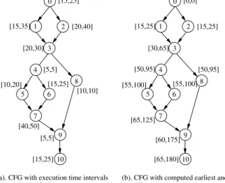
obtain for every task represented by its control-flow graph (see Figure 1.a), the interval of time [smin
b , emaxb ] during which every
basic block b might execute, considering the execution of τi in
isolation.
Computing execution intervals on loop-free code requires to know for every basic block b its earliest and latest start offsets sminb and smaxb . This can be done by a breadth-first traversal of
the CFG, applying to every traversed basic block b the following formulas: sminentry def = smaxentry def = 0 (1) sminb def = min x∈pred(b)(s min x + eminx ) (2) smaxb def = max x∈pred(b)(s max x + emaxx ) (3)
offsets per basic block 0 1 2 3 4 5 6 7 8 9 10
(b). CFG with computed earliest and latest start [0,0] [15,25] [15,25] [30,65] [55,100] [65,125] [50,95]
(a). CFG with execution time intervals per basic block
0 1 2 3 4 5 6 7 8 9 10 [15,25] [15,25] [20,40] [15,35] [20,30] [10,10] [40,50] [5,5] [5,5] [10,20] [60,175] [65,180] [50,95] [55,100] [15,25]
Fig. 1. Example of CFG for loop-free code. The CFG is composed of several basic blocks (0..10) connected by directed edges that represent jumps in the code. Each basic block is a set of sequential instructions delimited by a jump. In the left part, intervals [cmin
b , cmaxb ]represent the minimum and maximum execution times of basic block b. In the right part, intervals [smin
b , smaxb ]represent the earliest and latest start time of every basic block b.
with pred(b) the direct predecessor(s) of a basic block b in the CFG, and entry the task entry basic block. In the formulas, emin
x
(resp. emax
x ) represents the minimum (resp. maximum) execution
time of basic block x; such values can be produced by standard WCET estimation tools. Figure 1.b) shows for every basic block its earliest and latest start offset after applying the above formulas. Then, the time interval within which every basic block b may execute is [smin
b , sminb + emaxb ].
This method can be extended in a straightforward manner to programs with natural loops. The algorithm presented above can be applied to every loop individually, starting with the innermost. A loop can then be considered as a single node with known earliest and latest start offsets when analyzing the outer loop of the whole program. Similarly, tasks containing function calls can be analyzed provided that their call graph is acyclic by first analyzing the leaves in the call graph.
Knowing the possible execution interval [smin
b , emaxb ] of every
basic block b, the set of basic blocks that might execute at a given time instant t, noted BB(t) is known. For each basic block b in this set, state of the art methods like the one described in [3] is used to compute the maximum CRPD when preempting the task in basic block b, noted CRPDb. More formally, function fi can
be defined as follows: fi(t)
def
= max
∀b∈BB(t)(CRPDb)
V. DETERMINATION OFPREEMPTIONDELAYUPPER-BOUNDS
As stated in Section III, a task will always execute non-preemptively for at least Qitime units before a preemption occurs,
unless it completes before the end of the non-preemptive region. A naive thought to upper-bound the cumulative preemption delay over a task’s execution (say τi) might be to select from
fi the maximum number of points pk (each distanced from every
other by at least Qi time units) such that the sum �∀pkfi(pk)
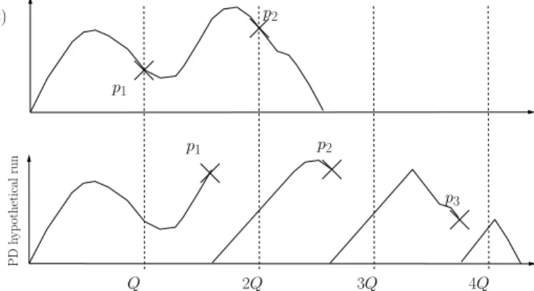
is maximum. However, the simple example depicted in Figure 2 shows that this solution is not correct. As we can see, on the top
p1 f (t) P D hy p oth eti ca l ru n p1 p2 p2 p3 Q 2Q 3Q 4Q
Fig. 2. Comparison Between Function fi and the Run-time Preemption Delay Development
plot where fiis depicted, there are at most two points that may be
selected (since no three points could be distanced by at least Qi
time units in time). The bottom plot presents an hypothetical run of task τi, where the run-time preemption delay cost is presented.
At run-time, since time is spent paying preemption delay after each preemption, more points can be selected (see the bottom plot), hence providing a higher cumulative preemption delay.
A pessimistic, but correct, solution to upper-bound the execu-tion time C�
iof a task τiwhile taking into account all the possible
preemption delays that τi might undergo during its execution, is
simply to multiply the maximum number of preemptions that can occur during τi’s execution (i.e.,
�
Ci
Qi
�
, this is discussed in more detail in [12]) by the maximum delay of one preemption (i.e., maxt∈[0,Ci]fi(t)). Given the increase in the WCET due to this
cumulative overhead, the maximum number of preemptions that can occur eventually increases as well. Therefore, this computa-tion has to be performed iteratively, in the style of the well-know task response-time computation, i.e., C�(0)
i = Ci and Ci�(k)= Ci+ � Ci�(k−1) Qi � × max t∈[0,Ci] fi(t) (4)
The pessimism of this computation comes directly from the fact that it considers a constant cost for every possible preemption, and this constant cost is assumed to be the maximum possible cost. That is, this approach is not sensitive to the preemption cost pattern of the task. As it was claimed in the abstract, using this additional information (the tasks preemption cost pattern) enables us to derive a much more accurate upper-bound. This second technique is described in Algorithm 1, and a detailed explanation is provided below.
Description of Algorithm 1. Initially we will explain the intuition of the approach on Figure 3 before presenting the actual algorithm. In Figure 3 the gray curve is the fi function.
Suppose that prog is the current progression in the task execution. Considering the next preemption point, the approach is looking for the lower bound on the progression which will be achieved within the next Qitime units in any preemption scenario. For this,
function fi is investigated from the current prog to prog +Qi.
On the ordinate also at length Qi a line D(x, t) is drawn to
prog +Qi. The point p∩ where f first crosses D(x, t) limits the
range of values which need to be considered. A preemption past this value would lead to a situation where this point would again
Algorithm 1: Upper-Bound the Preemption Delay
Input : fi(): preemption delay function of task τi Qi: length of the non-preemptive region
Output: total delay: cumulative preemption delay suffered by τi 1 prog← 0 ;
2 total delay← 0; 3 delaymax← 0 ; 4 pnext← Qi;
/* While the next progression is not beyond Ci */ 5 while pnext< Cido
/* Update time, progression and delay */
6 prog← pnext;
/* Compute the next progression step and the
next delay to account for */
7 p∩← min{px} such that
8 px∈ [prog(k), prog(k)+Qi] 9 and fi(px) =−px+ prog(k)+Qi} ; 10 if p∩= nullthen p∩← prog +Qi;
11 pmax← arg maxpx∈[prog,p∩]{fi(px)}; 12 delaymax← fi(pmax);
13 pnext← prog +Qi− delaymax; 14 total delay← total delay + delaymax; 15 return total delay ;
be considered in a subsequent iteration, since then prog would not pass this point in the current iteration. Within the interval, delaymax is determined. That means in an interval Qi under any
preemption scenario at least Qi− delaymax progress in program
execution will be achieved. It is a conservative bound as a later preemption means that also the non preemptible region will only start then. This point prog +Qi− delaymax will serve as new
starting point.
Returning to the Algorithm 1: Lines 1–4 initialise the variables. The variable prog memorizes the current progression in the task’s operations while total delay records the cumulative preemption delay accounted for up to the current progression. As the task τi executes, it accounts for progressing in its execution (and the
variable prog is increased) and for the preemption delay (which updates the variable total delay). The algorithm is iterative, and at each iteration the variables delaymaxand pnext (lines 3 and 4)
are the preemption delay taking place only in the current iteration and the next progression point in τi’s execution at which the next
iteration will start, respectively. Lines 1–4 can be seen as the first iteration of the algorithm. delaymax is set to 0 and pnext to Qi,
prog+ Qi pmax prog D(x, t) p∩ pnext delaymax Qi−delaymax delaymax Qi
because no preemption can occur during the first Qi time units
of τi’s execution.
The algorithm starts iterating at line 5, and it iterates as long as the next computed progression point pnext does not fall beyond
τi’s execution boundary. Line 6 shifts the current progression point
of τi to the computed value pnext. Then, lines 12 and 13 compute
the next progression point pnext and the maximum delay that τi
could suffer while progressing in its operations from its current progression point to pnext. Finally, line 14 adds this maximum
delay to the current cumulative delay accounted so far.
In the following Theorem 1, we prove that the value returned by Algorithm 1 is an upper-bound on the cumulative preemption delay that the given task τi might suffer during its execution.
This implies that the WCET of τi (while taking into account
all the possible preemption delays that τi might suffer during its
execution) is given by
Ci� def
= Ci+ total delay (5)
where total delay is the value returned by Algorithm 1. Theorem 1. Algorithm 1 returns an upper-bound on the preemp-tion delay that a given task τi can suffer during the execution of
any of its jobs.
Proof: Algorithm 1 computes the maximum cumulative pre-emption delay iteratively, by progressing step by step through the execution of the task τi. Hereafter, we use the notation prog(k) to
denote the progression through τi’s execution at the beginning of
the kth iteration of the algorithm. Similarly, total delay(k) will
be used to denote the cumulative preemption delay that τi has
suffered until it reached a progression of prog(k). In this proof, we
show that at each iteration k > 0, total delay(k)actually provides
an upper-bound on the cumulative preemption delay that τimight
suffer before reaching a progression of prog(k) in its execution.
The proof is made by induction.
Basic step. Algorithm 1 first considers that τi progresses by Qi
time units in its execution without suffering any preemption delay (since it cannot get preempted during these first Qi time units).
We consider this first step as the first iteration of the algorithm. That is, straightforwardly, total delay(1) = 0 is an upper (and
even exact) bound on the cumulative preemption delay that τi
may suffer before reaching a progression of Qi time units in its
execution.
Induction step. We assume (by induction) that total delay(k),
k > 1, is an upper-bound on the cumulative preemption delay that τi might suffer before reaching a progression of prog(k) time
units in its execution.
During the kthiteration, Algorithm 1 computes prog(k+1) and
total delay(k+1) as follows:
prog(k+1) = prog(k)+Qi− delaymax (6)
total delay(k+1) = total delay(k)+ delaymax (7)
where
delaymax = fi(pmax) (8)
pmax = arg max px∈[prog(k),p∩]
{fi(px)} (9)
p∩ = min{px} such that (10)
px∈ [prog(k), prog(k)+Qi]
and fi(px) =−px+ prog(k)+Qi
Equations 6 and 7 can be interpreted as follows. During the kth
iteration, Algorithm 1 assumes that τi executes for Qi time units
during which τi progresses by Qi− delaymax units of time in its
execution and suffers from a delay of delaymax; The algorithm
assumes that τi gets preempted when its progression reaches
pmax given by Equation 9. Below we show that choosing any
other preemption point pother �= pmax would ultimately1 result
in a cumulative preemption delay lower than the one returned by Algorithm 1, thus showing that the value returned by Algorithm 1 is an upper-bound. Two cases may arise: pother > pnext or
pother≤ pnext.
Case 1: pother > pnext. This means that τi progresses in its
execution until it reaches pnextwithout being preempted, i.e., from
a progression of prog(k), τ
i reaches a progression of pnext by
being executed only for (pnext− prog(k))time units, and with an
unchanged cumulative preemption delay of total delay(k). On
the other hand, in the execution scenario built by Algorithm 1, τi’s execution reaches a progression of prog(k+1) = pnext by
being executed for Qitime units, and with a cumulative
preemp-tion delay of total delay(k+1) = total delay(k)+ delay max ≥
total delay(k). In other words, Algorithm 1 manages to progress slower in τi’s execution while suffering from a greater preemption
delay. Furthermore, potheris still a candidate preemption point for
a further iteration of Algorithm 1.
Case 2. pother ≤ pnext. After executing τi for Qi time units,
we have that
1) the delay of the preemption that occurs when τi’s
progres-sion reaches pother has been totally accounted for (since
pother< pnext≤ p∩).
2) the progression of τi in this scenario becomes
progother = prog(k)+Qi− fi(pother)
≥ prog(k)+Qi− fi(pmax)
≥ prog(k+1) (11)
3) the cumulative preemption delay becomes total delayother = total delay
(k)
+fi(pother)
≤ total delay(k)+fi(pmax)
≤ total delay(k+1) (12) Thus, after executing τi for Qi time units Algorithm 1 progressed
less in the execution of τi (Inequality 11) while suffering from
a higher preemption delay (Inequality 12). As a consequence of Cases 1 and 2, it holds at each iteration of Algorithm 1 that choosing to preempt the task when it reaches a progression of pmax ultimately leads to an upper-bound on its cumulative
preemption delay.
1when τ
0 500 1000 1500 2000 2500 3000 3500 4000 −2 0 2 4 6 8 10 12 14 t
Preemption Delay Functions f
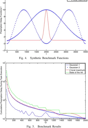
Gaussian 1 Gaussian 2 2 local maximum
Fig. 4. Synthetic Benchmark Functions
0 200 400 600 800 1000 1200 1400 1600 1800 2000 101 102 103 104 Q
Cumulative Preemption Delay During Task Execution
Gaussian 1 Gaussian 2 2 local maximum State of the Art
i
Fig. 5. Benchmark Results
VI. EVALUATION ANDDISCUSSION
Three synthetic fi functions have been created in order to
compare the performance of the proposed preemption delay estimation with the state-of-the-art method using the procedure described by Equation 4. The three functions used are two bell shaped functions, the first one with σ2= 300 and µ = 2000 and
a vertical offset of 10 units and the second one with a bigger variance, σ2 = 3000, the same average and no offset. Finally a
function with two local maxima separated in time is used. All functions have maximum value of 10 units, and have C = 4000. We vary the Qi value so having a fixed C still paints a generic
picture of how the methods behave.
The synthetic functions used represent distinct generic memory usage patterns from tasks. The sole purpose of the set of functions provided is to validate the method proposed in this paper. Having generic patterns, rather than function fi extracted from a set of
real benchmarks (which would present more complex patterns), enables for a more clear evaluation of Algorithm 1 performance. These functions are portrayed in Figure 4.
The proposed algorithm is shown empirically, in Figure 5, to provide a considerably less pessimistic upper-bound on the preemption delay value for a task, specially for smaller values of Qi. Since the state of the art method purely relies on Qi, Ci and
the maximum preemption delay of fi then its preemption delay
estimate is strictly the same for all the benchmark functions, since they all have the same C and maximum value. The preemption
delay axis in Figure 5 is in logarithmic scale so that the differences between the state of the art and the proposed algorithm are more easily observed across the entire Qi spectrum.
There are fluctuations in the results which are analysis artifacts and imply that the analysis is pessimistic. In some cases increasing the Qi results in bigger preemption delay. This is caused as
the analysis checks for the preemption delay in the window of prog and tA, but conservatively considers the actual preemption
to occur at prog. An actual preemption at pmax in physical
terms would initiate a new window of length Qi to start only
at that pmax instead of prog , thus the method, as is proven in
Theorem 1, provides an upper bound for the preemption delay in any conceivable real task execution scenario.
VII. CONCLUSION ANDFUTUREWORK
In this work we have proposed a new algorithm to compute an upper-bound on the preemption delay suffered by a task which executes in a system scheduled with preemption triggered floating non-preemptive regions. This algorithm has been shown to dominate over the state-of-the-art method. The method is easy to implement with small overhead and builds up on existing static-analysis methods.
As of future work we intend to tighten our result by (i) discarding less information during the computation of function fi(t)and (ii) reducing the number of preemptions (i.e., the number
of iterations) considered in Algorithm 1 – it is indeed impossible for a task to get preempted every Qi time units as assumed by
Algorithm 1 unless the periods of the other tasks enable such a preemption scenario.
REFERENCES
[1] S. M. Petters and G. F¨arber, “Scheduling analysis with respect to hardware related preemption delay,” in Workshop on Real-Time Embedded Systems, London, UK, Dec 2001.
[2] M. Bertogna and S. Baruah, “Limited preemption edf scheduling of sporadic task systems,” IEEE Transactions on Industrial Informatics, vol. 6, no. 4, Nov 2010.
[3] C.-G. Lee, J. Hahn, Y.-M. Seo, S. L. Min, R. Ha, S. Hong, C. Y. Park, M. Lee, and C. S. Kim, “Analysis of cache-related preemption delay in fixed-priority preemptive scheduling,” IEEE Transactions on Computers, vol. 47, no. 6, 1998.
[4] H. Ramaprasad and F. Mueller, “Bounding preemption delay within data cache reference patterns for real-time tasks,” in 12th RTAS, Apr 2006. [5] J. Busquets-Mataix, J. Serrano, R. Ors, P. Gil, and A. Wellings, “Adding
instruction cache effect to schedulability analysis of preemptive real-time systems,” in 17th RTSS, Jun 1996.
[6] S. Altmeyer, R. I. Davis, and C. Maiza, “Pre-emption cost aware response time analysis for fixed priority pre-emptive systems,” in 32nd RTSS, Nov 2011.
[7] L. Ju, S. Chakraborty, and A. Roychoudhury, “Accounting for cache-related preemption delay in dynamic priority schedulability analysis,” in 44th DATE, Apr 2007.
[8] A. Burns, “Preemptive priority-based scheduling: an appropriate engineering approach,” in Advances in real-time systems, S. H. Son, Ed. Upper Saddle River, NJ, USA: Prentice-Hall, Inc., 1995.
[9] Y. Wang and M. Saksena, “Scheduling fixed-priority tasks with preemption threshold,” in 6th RTCSA, 1999.
[10] G. Yao, G. Buttazzo, and M. Bertogna, “Comparative evaluation of limited preemptive methods,” in 15th ETFA, Sep 2010.
[11] ——, “Feasibility analysis under fixed priority scheduling with limited preemptions,” Journal Real-Time Systems, vol. 47, no. 3, 2011.
[12] J. Marinho and S. M. Petters, “Job phasing aware preemption deferral,” International Conference on Embedded and Ubiquitous Computing 2011, Oct 2011.
[13] M. Bertogna, O. Xhani, M. Marinoni, F. Esposito, and G. Buttazzo, “Optimal selection of preemption points to minimize preemption overhead,” in 23th RTSS, Jun 2011.