Science Arts & Métiers (SAM)
is an open access repository that collects the work of Arts et Métiers Institute of Technology researchers and makes it freely available over the web where possible.
This is an author-deposited version published in: https://sam.ensam.eu Handle ID: .http://hdl.handle.net/10985/12814
To cite this version :
Pierre GILORMINI, Jacques VERDU - On the role of hydrogen bonding on water absorption in polymers - Polymer - Vol. 142, p.164-169 - 2018
Published in Polymer vol. 142, pp. 164-169 (2018)
ON THE ROLE OF HYDROGEN BONDING
ON WATER ABSORPTION IN POLYMERS
Pierre Gilormini1 and Jacques Verdu
Laboratoire PIMM, ENSAM, CNRS, CNAM, 151 Bd de l'Hôpital, 75013, Paris, France
ABSTRACT. A kinetic model is proposed for the absorption of water in polymers. The process of bonding-debonding water molecules is described by two opposite reactions with different rate constants, and the key role of the concentration of traps by hydrogen bonding in the polymer matrix is highlighted. These three parameters are combined such that an equation is obtained that generalizes the model proposed by Carter and Kibler, with an additional, crossed, term. Numerical application is performed for the diffusion-absorption of water in a plane polymer sheet, and the parameter ranges where a quasi-Fickian water uptake curve is obtained are defined. The associated apparent diffusivity is shown to obey a hyperbolic variation with equilibrium water uptake for homologous series of polymers, which is in agreement with previous experimental observations.
KEYWORDS. Water absorption; Diffusion; Hydrogen bonding 1 Corresponding author.
1. Introduction
The absorption of water by a polymer sample results from a sequence of two distinct processes: water dissolution in a superficial polymer layer, which can be considered as almost instantaneous, and water diffusion into the sample core, which is driven by the gradient of chemical potential.
First, let us consider water solubility. A first type of theories on the relationship between structure and solubility links the capability of a polymer to absorb water to its free volume content [1,2]. This is consistent with the fact that the crystalline phase does not absorb water in a semi-crystalline polymer, but many free-volume rich substances absorb very small amounts of water, like apolar liquids or elastomers for instance. A way to reconcile these observations is to consider that free volume is needed for water diffusion, but does not play a role in solubility. A second kind of theories [3,4] involves the role of polar groups that can establish relatively strong hydrogen bonds with water molecules. This is supported, in particular, by a wide survey of water solubility values that allows to distinguish four polymer families: family A (polymers with low polarity, e.g., hydrocarbon polymers such as polyethylene, polypropylene, polystyrene, halogenated polymers such as polytetra-fluorethylene, poly(vinylidene fluoride), poly(vinyl chloride), polyalkylsiloxanes, etc.), family B (moderately polar polymers such as poly(ethylene terephthalate), bisphenol A polycarbonate, poly(methyl methacrylate), polyamide 11, polysulfones, etc.), family C (polar polymers such as polyetherimides, etc.), and family D (polymers with high concentrations of polar groups able to act as hydrogen donors in hydrogen bonds, such as polyamide 6, amine crosslinked epoxies of high alcohol content, etc.). The order of magnitude of water uptake mass fraction at equilibrium is below 0.3% for family A, between 0.3 and 2% for family B, between 2 and 5% for family C, and above 5% for family D. Another evidence favoring this
concentrations in families of polymers that differ only by their concentration of a given polar group, for instance polyesters for ester groups [5], polysulfones for sulfone groups [6], or amine cured epoxies for alcohol groups [7]. In all these families, the water equilibrium concentration increases regularly with the concentration of polar groups. This trend led Van Krevelen and Hoftyzer [3] to assume that water absorption is a molar additive property, i.e., that each elementary group i in the polymer is characterized by its molar contribution Hi to water equilibrium content, with Hi independent of the polymer structure. The molar equilibrium water content H in a given constituent repeat unit (CRU) would then simply be the sum of the His found in the CRU. Typical orders of magnitude of Hi at saturation are less than 0.01 moles water per mole CRU for hydrocarbon and halogenated groups, about 0.1 for such polar groups as ethers, ketones or esters, which are unable to establish hydrogen bonds with themselves, and between 1 and 2 for such groups as alcohols, acids or amides able to act as hydrogen donors in hydrogen bonds. The quantitative relationship between polymer structure and water solubility is probably more complex than a mere molar additive rule [6,7] but, no doubt, water solubility is closely related to the content of polar groups in the polymer and to the strength of the hydrogen bonds that they are able to establish with water molecules. Not all polar sites are able to establish a complex with a water molecule, and only those able to give a complex will be considered in what follows; these active sites will be called "traps".
Now, let us consider water diffusion. Its relationship with polymer structure has been investigated much less than for solubility. As mentioned above, diffusion needs free volume to operate, but it also depends on polymer-water interactions, as was first observed in the case of polyethylene [8] and for several polymer families afterwards, for which a quasi-hyperbolic relationship was found between diffusivity and water equilibrium concentration at saturation [9]. This result is consistent with the assumption that the bonds between traps and water molecules hinder water diffusion.
Therefore, according to the above set of observations, two kinds of water molecules coexist in a polymer sample exposed to a wet environment: mobile (free) molecules diffusing through the sample and bound (immobile) molecules temporarily delayed at traps by hydrogen bonds. This work will be limited to the case where free molecules can be captured at vacant traps only (no cluster formation) and, indeed, bound molecules can be released by the decomposition of polymer-water complexes. Therefore, the trajectory of a water molecule through a sample can be depicted as a series of random flights from one trap to another, with more or less long waiting times at these polar sites. Therefore, the global diffusion rate is expected to be a decreasing function of the concentration of traps and of the strength of polymer-water bonds.
Concerning the ratio between the concentrations of free water and bound water at equilibrium, a first indication can be derived from the study of homologous polymer series containing a single type of polar group, for instance sulfones in aromatic polysulfones as studied by Gaudichet-Maurin et al.[6]. These polymers can be described as matrices with low polarity containing highly polar sulfone groups whose volume fraction is relatively small. There is no reason to assume that the solubility and diffusivity of free water in these matrices vary strongly from one polysulfone to another. Bisphenol A polycarbonate, in which the unique polar group is an ester of low contribution to water absorption [8] is supposed to have water absorption properties close to those of aromatic polysulfones matrices. According to Table 1, the concentration of free water in these polymers would be less than 0.54%, i.e., less (and probably considerably less) than 50% of the whole water equilibrium concentration in the polysulfones. Similar observations could be inferred from series of aliphatic polyamides, where the best model for an apolar matrix would be polyethylene in which the equilibrium mass uptake would be less than 0.01% [8] against 5-10% for polyamides of the polyamide 6
type [6]. All these data lead to assume that the mass ratio between free water and bound water at equilibrium is considerably less than unity.
Polymer Sulfone concentration (mol/kg)
Equilibrium water mass uptake at 90% RH (%)
PSU 2.3 1.02
PPSU 2.5 1.58
PES 4.3 2.97
PC 0 0.54
Table 1. Concentration of sulfone groups and water equilibrium concentration in three aromatic polysulfones and in polycarbonate, according to Gaudichet-Maurin et al. [6].
Regarding now diffusion kinetics, it seems clear that a Langmuir-type model, as proposed by Carter and Kibler [10] and often used in the field of composite materials since the 80s (see for instance [11]), is a pertinent approach. Despite that, there are numerous cases of moderately hydrophilic polymers (in which plasticization and clustering effects are negligible, so that diffusivity is not concentration dependent) for which diffusion appears Fickian in a routine analysis based on the proportionality of mass uptake with respect to the square root of time up to 50% of equilibrium value or even on a visual comparison of the experimental sorption curve with a theoretical one, as illustrated by the examples of copolyamides [12], acrylic polymers [13], amine cured epoxies [14], or polysulfones [15].
(i) In which conditions does a Langmuir-type absorption-diffusion process lead to a quasi-Fickian water uptake curve?
(ii) When this applies, what is the relation between the resulting apparent diffusivity and the diffusivity of free water molecules in the polymer?
(iii) Does this relation reflect the quasi-hyperbolic dependence with respect to the equilibrium water uptake that is observed experimentally when polymers differ only by their concentration of a given polar group [9]?
2. Quasi-Fickian transport in the Carter and Kibler model
Forty years ago, Carter and Kibler [10] proposed a Langmuir-type model to describe anomalous (non-Fickian) diffusion of water in polymers, where trapped and mobile water molecules were accounted for. Introducing a probability per unit time 𝛾 for a mobile water molecule to bond, and a probability per unit time 𝛽 for a trapped water molecule to unbond, the model writes the following equation to govern the evolution of the local concentration 𝑐 of bound water (in moles per unit polymer mass):
= 𝛾 𝑐 − 𝛽 𝑐 (1)
where 𝑐 denotes the local concentration of mobile water. In the case of one-dimensional diffusion, as applies for instance in a plane sheet, the resulting balance of water molecules in a volume element writes as
𝐷 = + (2)
An analytical solution was given by Carter and Kibler to the system of coupled linear differential defined by Eq. (1) and Eq. (2) in the case of an initially dry sheet of thickness 𝑒 with a constant concentration of mobile water 𝑐 = 𝑐 prescribed on both free faces of the plate. The latter condition assumes that the ambience around the sheet is well-stirred and has a water activity unaffected by the amount of water absorbed by the specimen. The equilibrium, uniform, concentration 𝑐 of water in the plate, mobile plus bound, is readily deduced from Eqs. (1) and (2):
= 1 + (3)
where 𝛾/𝛽 is the relative contribution 𝑐 ⁄𝑐 of bound water. Note that 𝛾 can be positive or zero, but 𝛽 must be strictly positive, otherwise an endless water uptake would result because trapped water molecules cannot be released. The analytical solution involves an infinite sum of a complicated series to obtain either the total water uptake, or the mobile water uptake, or the bound water uptake, with respect to time. A simpler, approximate, solution was also provided by Carter and Kibler for the evolution of the total water uptake, or average water concentration 𝑐̅(𝑡), where the usual infinite series for Fickian diffusion is involved, with a limited validity in terms of 𝛽 and 𝛾 values. Our comparison between the exact and approximate solutions has shown that the latter is acceptable for 𝛽 and 𝛾 not greater than 0.02 (where = 𝐷 𝜋 /𝑒 ), which is a precise statement of the less definite rule (𝛽 and 𝛾 ≪ 0.5 ) given by Carter and Kibler. Therefore, the calculations reported below used the exact solution.
In the range where the approximate solution applies, the water uptake is strongly non-Fickian, in agreement with the initial purpose of the model, but a systematic analysis of the results obtained in larger ranges of 𝛽 and 𝛾 values shows that quasi-Fickian transport can also be obtained in addition to the purely Fickian case recovered exactly for any positive 𝛽 value
when 𝛾 = 0 (no bound water). Of course, the notion of a quasi-Fickian transport is quite arbitrary and must be defined precisely. In this study, ten √ 𝑡 values for water uptakes equal to 5%, 10%, 15%, ..., 50% of the equilibrium value were computed, and a linear least squares fit was applied to this set of (√ 𝑡, 𝑐̅/𝑐∞) pairs. This is similar to what might be done routinely when dealing with Fickian diffusion results where the very beginning of the experimental water uptake might be somewhat noisy and imprecise. According to the present definition, a quasi-Fickian transport is obtained if the standard deviation of 𝑐̅/𝑐∞ values is found less than one percent in the fitting procedure, and an apparent diffusivity 𝐷′ can then be deduced from the slope of the least-squares line. Figure 1 illustrates this notion of a quasi-Fickian transport with 𝛽⁄ = 0.25, 𝛾 ⁄ = 4.5, and 𝑐 ∞ = 1, where a standard deviation of 0.74% and an apparent diffusivity 𝐷 = 0.06 𝐷 have been obtained. The water uptake evolution given by the approximate solution is also shown in order to stress that it may lead to significant errors when used beyond its limited range of validity.
Figure 1. Example of a quasi-Fickian transport (solid line) given by the Carter and Kibler model with 𝛽⁄ = 0.25, 𝛾 ⁄ = 4.5, and 𝑐 = 1. The least-squares fitted line deduced from
the range shown is plotted (dotted line). For comparison, the water uptake given by the approximate expression of the exact solution is also plotted (dashed line).
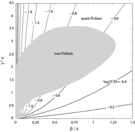
Figure 2 shows the domain where a quasi-Fickian transport is obtained with the Carter and Kibler model, and the associated apparent diffusivities. In this graph, the range of validity of the approximate solution is extremely small, a purely Fickian transport is obtained along the horizontal axis (𝛾 = 0), and a quasi-Fickian transport is obtained for sufficiently large 𝛾 and 𝛽 values, in particular. The apparent diffusivity 𝐷′ is found lower than the diffusivity 𝐷 of mobile water molecules, except along the horizontal axis, where 𝐷 = 𝐷 of course, and it decreases when the vertical axis is approached, which is consistent with the endless water uptake mentioned above when 𝛽 = 0. For a given polymer, i.e., for fixed 𝛾, 𝛽, and 𝐷, a decrease in the sheet thickness increases and therefore the (𝛽⁄ , 𝛾 ⁄) pair moves towards the origin of the graph along a straight line, which ends up necessarily with a non-Fickian transport. The decrease of 𝐷 /𝐷 when the sheet thickness increases illustrates that the apparent diffusivity is not a material parameter, in contrast to 𝐷 . This variation may nevertheless be moderate for limited thickness variations if the initial (𝛽⁄ , 𝛾 ⁄) pair is large enough, because of the almost radial shape of the 𝐷 /𝐷 contours in Figure 2.
Since 𝑐 ⁄𝑐 can increase indefinitely in Eq. (3) by increasing 𝛾 or decreasing 𝛽, none of these two parameters is able to display that a polymer has a definite absorption capacity that is independent from these probabilities per unit time and is limited by a given number of traps per unit polymer mass. This deficiency of the Carter and Kibler model, although questions (i) and (ii) given at the end of Section 1 could be addressed, has motivated the kinetic model that follows.
Figure 2. Map of log 𝐷′ 𝐷⁄ (values given on the contour lines) when a quasi-Fickian transport with diffusivity 𝐷′ is obtained from the Carter and Kibler model. The transport is
non-Fickian in the gray area where no contour line is shown.
3. A kinetic model for water absorption in polymers
The key component in the proposed kinetic model is a given concentration 𝑝 (in moles per polymer unit mass) of traps in the dry polymer that are able to establish a complex with a water molecule. The kinetics of bonding a water molecule 𝑊 at a trap 𝑃 to give a complex 𝑃𝑊 and of unbonding a water molecule from a complex 𝑃𝑊 can be described by two opposite reactions:
where 𝑘 is a second order rate constant (in mol kg-1 s-1) and 𝑘 a first order rate constant (in s-1). Therefore, the concentration of bound water molecules (or water complexes) at a given point in a polymer sample is governed by
= 𝑘 (𝑝 − 𝑐 ) 𝑐 − 𝑘 𝑐 = 𝑘 𝑝 𝑐 − 𝑘 𝑐 − 𝑘 𝑐 𝑐 (5)
in terms of the concentrations of mobile water and of traps, since the current concentration of traps that are available to bond additional water molecules is 𝑝 − 𝑐 . Thus, Eq. (5) leads to an extended variant of Eq. (1):
= 𝛾 𝑐 − 𝛽 𝑐 − 𝛿 𝑐 𝑐 (6)
where 𝛾 = 𝑘 𝑝, 𝛽 = 𝑘 , and 𝛿 = 𝑘 , with an additional and crossed term with respect to Eq. (1) of the Carter and Kibler model, where the role of a concentration of traps was ignored. Because the balance of water molecules in a volume element is unchanged formally, Eq. (2) still applies, and Eq. (6) together with Eq. (2) forms the core of the proposed kinetic model of water absorption in polymers for one-dimensional diffusion. It may be noticed that Eq. (6) is similar to the equation obtained fifty-five years ago by McNabb and Foster [16] for the non-Fickian diffusion of hydrogen in iron and ferritic steels by accounting for a limited population of traps. That paper has been largely unnoticed by the polymer community, even by Carter and Kibler [10], except by Yamabe et al. [17] and Beckman and Teplyakov [18] in the context of hydrogen absorption or permeation in polymers, for instance, or by Gurtin and Yatomi [19] and Dewimille and Bunsell [20] for water absorption. Nevertheless, these references used at most a simplified version of the model that amounts finally to the Carter and Kibler approach.
For an initially dry plate where a constant concentration of mobile water 𝑐 = 𝑐∞ is maintained on the free faces at 𝑥 = 0 and 𝑥 = 𝑒, the evolution of the concentration of bound water at the free faces is obtained immediately from Eq. (6) as
𝑐 (0, 𝑡) = 𝑐 (𝑒, 𝑡) = {1 − exp[−(𝛽 + 𝑐 𝛿)𝑡]} (7)
Therefore, the lifetime of a polymer-water complex is 1/(𝛽 + 𝑐 𝛿) and depends on the free water concentration, whereas a lifetime of 1/𝛽 is obtained with the Carter and Kibler model (𝛿 = 0). In other words, the decomposition of a polymer-water complex is as slow as the concentration of free water is large in the kinetic model. Moreover, the equilibrium concentration 𝑐 , mobile plus bound, is now given by
= 1 + (8)
where the contribution of bound water
𝑐 = = ⁄ ≤ 𝑝 (9)
is limited by the concentration 𝑝 of traps, whatever the positive values of the parameters 𝑘 , 𝑘 , and 𝑐 . This is physically sound and contrasts with the trend mentioned at the end of Section 2 about the Carter and Kibler model. As mentioned in Section 1, the concentration of bound water molecules at equilibrium in polymers is expected to be much larger than the concentration of mobile water molecules, and it will be assumed in what follows that 𝑐 ⁄𝑐 ≥ 10, i.e.:
𝛾 ≥ 10 (𝛽 + 𝑐∞ 𝛿) (10)
The pair of differential equations of the model, namely Eq. (6) and Eq. (2), is non linear because of the crossed term, and therefore it was solved numerically by applying a standard finite difference scheme (comparable to what Caskey and Pillinger [21] implemented for the McNabb and Foster model [16]) to obtain 𝑐 (𝑥, 𝑡) and 𝑐 (𝑥, 𝑡), with initial conditions 𝑐 (𝑥, 0) = 0 and 𝑐 (𝑥, 0) = 0, where 0 ≤ 𝑥 ≤ 𝑒 . For symmetry reasons, one half of the sheet thickness was considered, with a constant concentration 𝑐 = 𝑐∞ prescribed at the free
surface 𝑥 = 0 and mirror symmetry imposed to 𝑐 and 𝑐 at 𝑥 = 𝑒/2 . In addition to normalizing 𝛽 and 𝛾 by like in Section 2, 𝛿 was adimensionalized by dividing by ⁄𝑐∞. As a result, a computed adimensionalized total water uptake history 𝑐̅(√ 𝑡)/𝑐∞ is kept unchanged if the data are modified such that 𝛽⁄, 𝛾⁄ and 𝑐∞𝛿⁄ are unchanged. This allows analysis of the effects of the 6 parameters that come into play in the problem (𝑒, 𝐷, 𝑐∞, 𝛽, 𝛾, and 𝛿) by exploring a three-dimensional space of dimensionless parameters. Of course, the available analytical solutions for the Fickian case (𝛾 = 0) and for the Carter-Kibler case (𝛿 = 0) were used in preliminary tests to assess the precision of the numerical procedure. It may be noticed that taking 𝛿 = 0 in the kinetic model recovers the Carter and Kibler model formally only, since this would imply 𝑘 = 0 and consequently 𝑝 should tend to infinity to allow a finite 𝛾 value (otherwise the trivial Fickian case is recovered).
Once a water uptake history has been computed, it can be tested as described in Section 2 to check if it is quasi-Fickian or not, and an apparent diffusivity 𝐷′ is deduced if this is the case. In practice, since Eq. (10) is assumed to apply, the conditions for a quasi-Fickian transport were finally found equivalent to defining minimal 𝛾⁄ values in the (𝛽⁄ , 𝑐 ∞ 𝛿⁄ ) plane, and Figure 3 shows the results that were obtained. Note that the 𝛽⁄ = 0 axis corresponds to all traps being occupied by water molecules (𝑐∞ = 𝑝), according to Eq. (9). Recall that, in addition, the origin of the (𝛽⁄ , 𝑐 ∞ 𝛿⁄ ) plane should be excluded because of no stationary water uptake being reached. Figure 3 shows that a quasi-Fickian transport is always obtained if 𝛾⁄ is large enough, for a given (𝛽⁄ , 𝑐 ∞ 𝛿⁄ ) pair, but time to reach the equilibrium water uptake may then be extremely long. The condition stated by Eq. (10) is sufficient to define the minimum 𝛾⁄ value beyond the limits of Figure 3, since the plane that it defines is visualized by straight, parallel and equidistant contour lines. An example of a typical quasi-Fickian transport is shown in Figure 4 with 𝛽⁄ = 0.25, 𝛾 ⁄ = 4.5, 𝑐 ∞ 𝛿⁄ =
0.2, and 𝑐∞ = 1, where a standard deviation of 0.99% and an apparent diffusivity 𝐷 = 0.11 𝐷 have been obtained.
Figure 3. Map of minimal 𝛾⁄ values (given on contour lines) such that Eq. (10) is satisfied and a quasi-Fickian transport is observed, for any positive 𝛽⁄ and 𝑐∞ 𝛿⁄ values.
Figure 4. Example of a quasi-Fickian transport (solid line) given by the kinetic model with 𝛽⁄ = 0.25, 𝛾 ⁄ = 4.5, 𝑐 ∞ 𝛿⁄ = 0.2, and 𝑐 ∞ = 1.
The least-squares fitted line is also shown (dotted line).
The curve in Figure 4 can be split into a water uptake in the polymer sheet for bound molecules 𝑐̅ and a water uptake for mobile molecules 𝑐̅ , and the evolutions of these two components are shown in Figures 5 and 6. It can be observed in Figure 5 that the bound water uptake increases more slowly with our kinetic model than with the Carter and Kibler model and that a stationary state is obtained faster, with a smaller water concentration: this is a natural effect of parameter 𝛿 in Eqs. (6) and (9) (recall that 𝛿 = 0 in the Carter and Kibler model). The much higher level reached by the Carter and Kibler model in Figure 5 explains the differences of the equilibrium values obtained in Figures 1 and 4. In contrast, the same levels are obtained with both models for the mobile water uptake (Figure 6), since the same boundary condition of a constant concentration of mobile water has been applied to the sheet faces. Nevertheless, a stationary state is reached faster with our kinetic model, which can be related to the shorter lifetime of bound water discussed below Eq. (7). A two-stage mobile
to 𝐷, since it corresponds to a very low content in trapped water molecules (flat beginning of the curves in Figure 5) that also explains the coincidence with the Carter and Kibler model (negligible crossed term in Eq. (6)). The increasing role of bonding in the second stage reduces the flux of mobile molecules, lowers their apparent diffusivity, and makes the two models more dissimilar.
Figure 5. Bound water uptake (solid line) given by the kinetic model with 𝛽⁄ = 0.25, 𝛾 ⁄ = 4.5, 𝑐 ∞ 𝛿⁄ = 0.2, and 𝑐 ∞ = 1. The 𝛿 = 0 case
Figure 6. Mobile water uptake (solid line) given by the kinetic model with 𝛽⁄ = 0.25, 𝛾 ⁄ = 4.5, 𝑐 ∞ 𝛿⁄ = 0.2, and 𝑐 ∞ = 1. The 𝛿 = 0 case
(Carter and Kibler model) is also shown for comparison (dashed line).
4. Correlation between apparent diffusivity and water uptake
The aim of this Section is to explain the quasi hyperbolic dependence that is observed between the diffusion coefficient and the equilibrium water uptake for certain homologous or quasi homologous series of polymers [9]. It is noteworthy that the retarding role of hydrogen bonding on water diffusion was envisaged, more than 40 years ago, by Bramhall [22] in the case of wood; however this role was analyzed only from the point of view of thermodynamics in a case where no homologous series can be defined.
Consider a homologous series of polymers differing only by the concentration of a given polar group, e.g., amorphous aliphatic polyamides. These polymers have the same matrix, in which the mobile water equilibrium uptake and diffusivity can therefore be supposed constant. In contrast, the bound water uptake (and then the overall water uptake) is expected to increase with the concentration p of traps presumably sharply linked to the
concentration of polar groups, and the apparent diffusivity 𝐷 is expected to decrease. The trend of an increasing 𝑐 when 𝑝 increases has already been obtained above with the kinetic model through Eq. (9); therefore, 𝑐 increases with 𝑝 as well. The second trend of a decreasing 𝐷 can be analyzed through the results obtained with the kinetic model when 𝑝 is increased while 𝑘 , 𝑘 , 𝑐 and are kept constant. Equivalently, 𝛽⁄ and 𝑐∞ 𝛿⁄ are kept constant and 𝛾⁄ is increased in a range where a quasi-Fickian transport applies according to Figure 3. This has been performed in Figure 7 for three sets of parameter values and for a wide range of water uptakes (over more than one decade) in each case. It can be observed that a quite straight line is obtained for a given homologous series in a logarithmic plot of 𝐷 /𝐷 vs. the total water uptake 𝑐 , with a slope that is very close to −1. This is in very good agreement with the experimental results [9] reported in Section 1. Moreover, varying both 𝛽⁄ and 𝑐∞ 𝛿⁄ by a factor of 10 or 0.1 has essentially the effect of shifting the curve along itself, with a slight translation along the perpendicular direction, as shown in Figure 7. It may be added finally that varying either 𝛽⁄ or 𝑐∞ 𝛿⁄ by a factor of 10 or 0.1 has the same effect, and therefore, quite remarkably, the essential variations of 𝐷 /𝐷 vs. the total water uptake 𝑐 for any 𝛽⁄ and 𝑐∞ 𝛿⁄ values is described in Figure 7. Therefore, the apparent diffusivity in a polymer during water absorption can be approximated as follows:
≈ = =
/
(11) when a quasi-Fickian transport is observed and Eq. (10) applies.
Figure 7. Examples of the correlation between the water uptake 𝑐 and the apparent diffusivity 𝐷 given by the kinetic model when a quasi-Fickian transport is observed and Eq. (10) applies. 𝛽⁄ = 0.25, 𝑐 ∞ 𝛿⁄ = 0.2 (solid line), 𝛽 ⁄ = 2.5, 𝑐 ∞ 𝛿⁄ = 2 (dashed
line), and 𝛽⁄ = 0.025, 𝑐 ∞ 𝛿⁄ = 0.02 (dotted line), with 𝑐 = 1 in all cases.
5. Identification of model parameters
An identification procedure of the five parameters involved in the model, D, 𝑐 , 𝑝, 𝑘 , and 𝑘 (or, equivalently, D, 𝑐 , 𝛽, 𝛾 and 𝛿), may consider a series of homologous polymers, which allows deducing D and 𝑐 from the Fickian water uptake that applies in the case where p is close to 0. For a given polymer in the series, p can be bracketed between a lower value equal to the concentration of absorbed water (see Eq. (9)) and an upper value derived from the molecular structure of the polymer. As Eq. (11) suggests, the 𝑘 /𝑘 ratio can then be deduced from the apparent diffusivity or water uptake. Finally, parameter 𝑘 can be evaluated from the Arrhenius equation using a preexponential factor of the order of 10-13 s (i.e., the reciprocal of the period of a molecular vibration as applies to a unimolecular first order process) and an
activation energy equal to the dissociation energy of hydrogen bonds and thus equal to the heat of dissolution of water in the polymer. The latter is about 30 kJ/mol for polymers in family A [8] as listed in Section 1, between 30 and 40 kJ/mol for family B [23], between 40 and 43 kJ/mol for family C [23], and above 43 kJ/mol for family D [7].
An alternative or complementary identification strategy can also be considered if very thin polymer plates are available, since the beginning of the corresponding water uptake is identical to what is obtained with the Carter and Kibler model. Accordingly, D can be deduced from the initial slope of the curve and 𝑐 is given directly by the well-known intermediate plateau. According to (8), the equilibrium water uptakes obtained for various ambient moistures give the 𝛿/𝛾 and 𝛽/𝛾 ratios once 𝑐 is obtained in each case. Finally, a numerical fit of the model to a whole water uptake curve would lead to the last parameter needed, e.g., 𝛾.
6. Conclusion
A given polymer can be considered as a matrix of low polarity containing polar sites able to trap water molecules with strong hydrogen bonds to form complexes of finite lifetime. The process of bonding-debonding water molecules was described here by two opposite reactions with different rate constants, and the key role of the concentration of traps was highlighted. These three parameters could be combined such that an equation is obtained that generalizes the model proposed by Carter and Kibler, with an additional, crossed, term. Numerical application was performed for the diffusion-absorption of water in a plane polymer sheet, and the parameter ranges where a quasi-Fickian water uptake curve is obtained were defined. The associated apparent diffusivity was shown to obey a hyperbolic variation with equilibrium
water uptake for homologous series of polymers, which is in agreement with previous experimental observations.
This work opens a series of questions, among which the following ones:
(i) About equilibrium properties: is it possible to establish the relationships between the matrix structure (e.g., aliphatic, rubbery for polyethylene vs. aromatic, glassy for polysulfones) and its properties D and 𝑐 ? How to derive the sorption isotherm from the proposed kinetic model?
(ii) Our kinetic model is restricted to the case where no water clusters are formed: how to take them into account? This would lead to consider a series of equilibria for polymer-water complexes PW, PW2, PW3, etc., but how to estimate the values of the rate constants associated with each complex size?
(iii) Our approach assumes implicitly that all traps are identical, i.e., they have the same 𝛽 and 𝛾 values. However, a theory [6,7] suggests that a trap would actually be a pair of polar groups, and the energy involved when a water molecule is bonded would depend on the distance between the two polar groups. As a consequence, the lifetime of the corresponding complex, i.e., the 𝛽 value, would vary from one trap to another. This leads to the following question: how to define a pertinent distribution of 𝛽 values to generalize our model?
We think that the proposed kinetic model complemented with the answers to the above questions would constitute a significant step towards the understanding of water absorption mechanisms in polymers.
Acknowledgments
The authors are grateful to Y. Charles, from LSPM, Université Paris 13, France, for drawing their attention to the paper by A. McNabb and P.K. Foster.
References
[1] Adamson MJ. J Mater Sci 1980;15:1736-1745.
[2] Enns JB, Gilham JK. J Appl Polym Sci 1983;28:2831-2846.
[3] Van Krevelen DW, Hoftyzer PJ. Properties of Polymers. Their Correlation with Chemical Structure. Their Numerical Estimation and Prediction from Additive Group Contributions, 3rd ed., Elsevier, Amsterdam 1990.
[4] Barrie JA. in Diffusion in Polymers, J. Crank J. and G.S. Park eds, Academic Press, London 1968, 259-313.
[5] Bellenger V, Mortaigne B, Verdu J. J Appl Polym Sci 1990;41:1225-1233.
[6] Gaudichet-Maurin E, Thominette F, Verdu J. J Appl Polym Sci 2008;109:3279-3285. [7] Tcharkhtchi A, Bronnec PY, Verdu J. Polymer 2000;41:5777-5785.
[8] McCall DR, Douglass DC, Blyler LL, Edward-Johnson G, Jelinski LW, Bair HE. Macromolecules 1984;17:1644-1649
[9] Thominette F, Gaudichet-Maurin E, Verdu J. Defects and Diffusion Forum 2006;258-260:442-446
[10] Carter HG, Kibler KG. J Compos Mater 1978;12:118-130.
[11] Bunsell AR. in Developments in Reinforced Plastics, G. Pritchard ed., Applied Science Publishers, London, 3:1-24, 1984.
[12] Del Nobile MA, Buonocore GG, Palmieri L, Aldi A, Acierno DJ. Food Eng 2002;53: 287-293.
[13] Rodriguez O, Fornasiero F, Arce A, Radke CJ, Prausnitz JM. Polymer 2003;44:6323-6333.
[14] Damian C, Escoubes M, Espuche E. J Appl Polym Sci 2001;80:2058-2066. [15] Schult KA, Paul DR. J Polym Sci Part B: Polymer Physics 1996;34:2805-2817. [16] McNabb A, Foster PK. Trans Metal Soc AIME 1963;227:618-627.
[17] Yamabe J, Nishimura S, Nakao H, Fujiwara H. in Effects of Hydrogen on Materials, Proc. 2008 Int. Hydrogen Conf., B. Somerday, P. Sofronis, and R. Jones Eds, ASM International, 389-396, 2009
[18] Beckman IN, Teplyakov VV. Adv Colloids Interface Sci 2015;222:70-78. [19] Gurtin ME, Yatomi C. J Compos Mater 1979;13:126-130.
[20] Dewimille B, Bunsell AR. J Phys D: Appl Phys 1982;15:2079-2091. [21] Caskey GR, Pillinger WL. Metall Trans A 1975;6A:467-476.
[22] Bramhall G. Wood Sci 1976;8:153-161.