A TL-SOFT -PUB-2018-001 12 July 2018
ATLAS PUB Note
ATL-SOFT-PUB-2018-001
10th July 2018Deep generative models for fast shower simulation
in ATLAS
The ATLAS Collaboration
The need for large scale and high fidelity simulated samples for the extensive physics program of the ATLAS experiment at the Large Hadron Collider motivates the development of new simulation techniques. Building on the recent success of deep learning algorithms, Vari-ational Auto-Encoders and Generative Adversarial Networks are investigated for modeling the response of the ATLAS electromagnetic calorimeter for photons in a central calorimeter region over a range of energies. The properties of synthesized showers are compared to showers from a full detector simulation using Geant4. This feasibility study demonstrates the potential of using such algorithms for fast calorimeter simulation for the ATLAS experiment in the future and opens the possibility to complement current simulation techniques. To em-ploy generative models for physics analyses, it is required to incorporate additional particle types and regions of the calorimeter and enhance the quality of the synthesized showers.
© 2018 CERN for the benefit of the ATLAS Collaboration.
1 Introduction
The extensive physics program of the ATLAS experiment [1] at the Large Hadron Collider [2] relies on
high-fidelity Monte Carlo (MC) simulation as a basis for hypothesis tests of the underlying distribution of the data. One of the key detector technologies used for characterizing collisions are calorimeters, measuring the energy and location of both charged and neutral particles traversing the detector. Particles will lose their energy in a cascade (called a shower) of electromagnetic and hadronic interactions with a dense absorbing material. The number of the particles produced in these interactions is subsequently measured in thin sampling layers of an active medium.
The deposition of energy in the calorimeter due to a developing shower is a stochastic process that can not be described from first principles and rather relies on a precise simulation of the detector response. It requires the modeling of interactions of particles with matter at the microscopic level as implemented
using the Geant4 toolkit [3]. This simulation process is inherently slow and thus presents a bottleneck in
the ATLAS simulation pipeline [4].
To meet the growing analysis demands, ATLAS already relies strongly on fast calorimeter simulation techniques based on thousands of individual parametrizations of the calorimeter response in the
longit-udinal and transverse direction given a single particle’s energy and pseudorapidity [5]. The algorithms
currently employed for physics analyses by the ATLAS collaboration achieve a significant speed-up over
the full simulation of the detector response at the cost of accuracy. Current developments [6, 7] aim at
improving the modeling of taus, jet-substructure-based boosted objects or wrongly identified objects in the calorimeter and will benefit from an improved detector description following data taking and a more detailed forward calorimeter geometry.
In recent years, deep learning algorithms have been demonstrated to accurately model the underlying distributions of rich, structured data for a wide range of problems, notably in the areas of computer vision, natural language processing and signal processing. The ability to embed complex distributions in a low dimensional manifold has been leveraged to generate samples of higher dimensionality and approximate the underlying probability densities. Among the most promising approaches to generative models are
Variational Auto-Encoders (VAEs) [8,9] and Generative Adversarial Networks (GANs) [10], shown to
simulate the response of idealized calorimeters [11–13].
This note presents the first application of such models to the fast simulation of the calorimeter response of the ATLAS detector, demonstrating the feasibility of using such algorithms for large scale high energy physics experiments in the future, and opens the possibility to complement current techniques. The studies presented in this note focus on generating showers for photons over a range of energies in the central region of the electromagnetic calorimeter. These showers are easier to reproduce and thus studied first, in particular the longitudinal and lateral shower shapes. Through the simplifications made, it is possible to focus on narrow regions of the calorimeter and neglect the dependence of the calorimeter response on the incident particle’s pseudorapidity. Furthermore, the extension of the algorithms for different particle types through conditioning the models on these types, is not studied.
The note is organized as follows. Section2describes the design of the ATLAS detector and the geometry
of the calorimeter system in particular. The Monte Carlo simulation samples used are described in
Section3. Section4presents a comprehensive summary of the deep generative models exploited in this
work as well as their optimization. The results obtained by these algorithms are reviewed in Section5.
2 ATLAS calorimeter
The ATLAS experiment at the LHC is a multipurpose particle detector with a forward-backward symmetric cylindrical geometry, covering nearly hermetically the full 4π solid angle by combining several
sub-detector systems installed in layers around the interaction point1.
The inner tracker, covering the pseudorapidity range |η| < 2.5, consists of silicon pixel and silicon microstrip tracking detectors inside a transition-radiation tracker, immersed in a 2 T axial magnet field provided by a thin superconducting solenoidal coil. For run 2 of the LHC, it includes a newly installed innermost silicon pixel layer, the insertable B-layer.
Lead/liquid-argon (LAr) sampling calorimeters with an accordion geometry in φ direction, i.e. accordion-shaped kapton electrodes and lead absorber plates with varying size in different regions of the detector,
as shown in Fig.1. This geometry allows modules to overlap each other and avoid intermodule gaps.
The design provides electromagnetic (EM) energy measurements for |η| < 2.5 with high granularity and longitudinal segmentation into multiple layers, capturing the shower development in depth. In the following, front, middle and back refer to the three layers in the central region of the EM barrel. In the region of |η| < 1.8, the ATLAS experiment is equipped with a LAr presampler detector to correct for the energy lost by electrons and photons upstream of the calorimeter and thus to improve the energy measurements in these regions. The EM calorimeter is surrounded by a hadronic sampling calorimeter consisting of steel absorbers and active scintillator tiles, covering the central pseudorapidity range (|η| < 1.7).
The EM endcap is instrumented using the same fine granularity LAr calorimeters and lead absorbers, while the hadronic endcap utilizes copper absorbers with reduced granularity. The coverage up to |η| < 4.9 is completed with forward copper/LAr and tungsten/LAr calorimeter modules, optimized for electromagnetic and hadronic measurements respectively.
The ATLAS calorimeter is segmented into a matrix of three dimensional cuboids with varying shape and size in the r/z, η, φ space (x, y, z space for the forward calorimeters). The EM calorimeter is over 24 interaction lengths in depth, ensuring that there is little leakage of EM showers into the hadronic calorimeter. The total depth of the complete calorimeter is over 9 interaction lengths in the barrel and over 10 interaction lengths in the endcap, such that good containment of hadronic showers is obtained. The muon spectrometer surrounds the calorimeters and is based on three large air-core toroid supercon-ducting magnets with eight coils each. The field integral of the toroids ranges from 2.0 to 6.0 T m across most of the detector. It includes a system of precision tracking chambers (|η| < 2.7) and fast detectors for triggering (|η| < 2.4).
The detailed structure of the calorimeter system influences the architecture of the deep generative models for fast simulation of signals in the calorimeters presented in this note. Out of the EM barrel layers, the middle layer is the deepest and receives the maximum energy deposit from EM showers. The front layer is thinner and exhibits a fine granularity in |η| < 1.4 (eight times finer than the middle layer), but four times less granular in φ. In the back layer less energy is deposited compared to the front and middle layers.
1ATLAS uses a right-handed coordinate system with its origin at the nominal interaction point (IP) in the centre of the detector and the z-axis along the beam pipe. The x-axis points from the IP to the centre of the LHC ring, and the y-axis points upwards. Cylindrical coordinates (r, φ) are used in the transverse plane, φ being the azimuthal angle around the z-axis. The pseudorapidity is defined in terms of the polar angle θ as η = − ln tan(θ/2). Angular distance is measured in units of ∆R ≡p(∆η)2+ (∆φ)2.
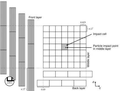
0.025 π/27
0.05 π/25
Impact cell
Particle impact point in middle layer Middle la yer Back layer Front layer φ η 0.025/8
0.025
π
/2
7
0.05
π
/2
5
Impact cell
Particle impact point
in middle layer
Middle
la
yer
Back layer
Front layer
φ
η
0.025/8Figure 1: Illustration of possible alignments in φ for the front layer, (left, showing a 8 × 3 portion of the 56 × 3 cell image) and the back layer (bottom, showing a 4 × 1 portion of the 4 × 7 cell image) with respect to the middle layer (center, showing the full 7 × 7 image). The front (back) layer are visualized to the left (bottom) of the middle layer to illustrate the alignments in φ (η), but are actually one behind another in the third dimension.
3 Monte Carlo samples and preprocessing
The ATLAS simulation infrastructure, consisting of event generation, detector simulation and digitization, is used to produce and validate the samples used for the studies presented in this note. Samples of single unconverted photons are simulated using Geant4 10.1.patch03.atlas02, the standard MC16 RUN2 ATLAS geometry (ATLAS-R2-2016-01-00-01) with the conditions tag OFLCOND-MC16-SDR-14. The simulation
employs the FTFP_BERT physics list [14], i.e. uses the Geant4 Bertini-style cascade [15–17] to simulate
hadron-nucleus interactions at low incident hadron energies, and the Fritiof parton string model [18,19]
at higher energies, followed by the Geant4 precompound model to de-excite the nucleus. Specific to the version used by ATLAS is that the handover between the models is performed in the energy region between 9 GeV and 12 GeV.
The samples are generated for nine discrete particle energies logarithmically spaced in the range between approximately 1 and 260 GeV and uniformly distributed in 0.20 < |η| < 0.25. The truth particles are generated on the calorimeter surface, i.e. the handover boundary between inner detector and the calorimeter in the integrated simulation framework. Thus, the showers are not subject to energy losses in the inner detector and the cryostat/solenoid magnet. Each simulated sample contains up to 10000 generated events, totaling approximately 90000 events. The generated samples do not include displacements corresponding to the expected beam spread of the ATLAS interaction region. Alongside the energy deposited in the calorimeter cells, the detailed spatial position of each energy deposit is saved. In the digitization of the Geant4 hit output, electronic noise, cross talk between neighbouring cells and dead cells are turned off. Cell energies are required to be positive. Overlapping showers in this setup do not exactly factorize. The showers originating from photons deposit almost their entire energy in the EM calorimeter and show little leakage into the hadronic calorimeter. Therefore only layers of the EM calorimeter are considered. Considering calorimeter cells as cuboids, for each layer the energy deposits within a rectangular selection
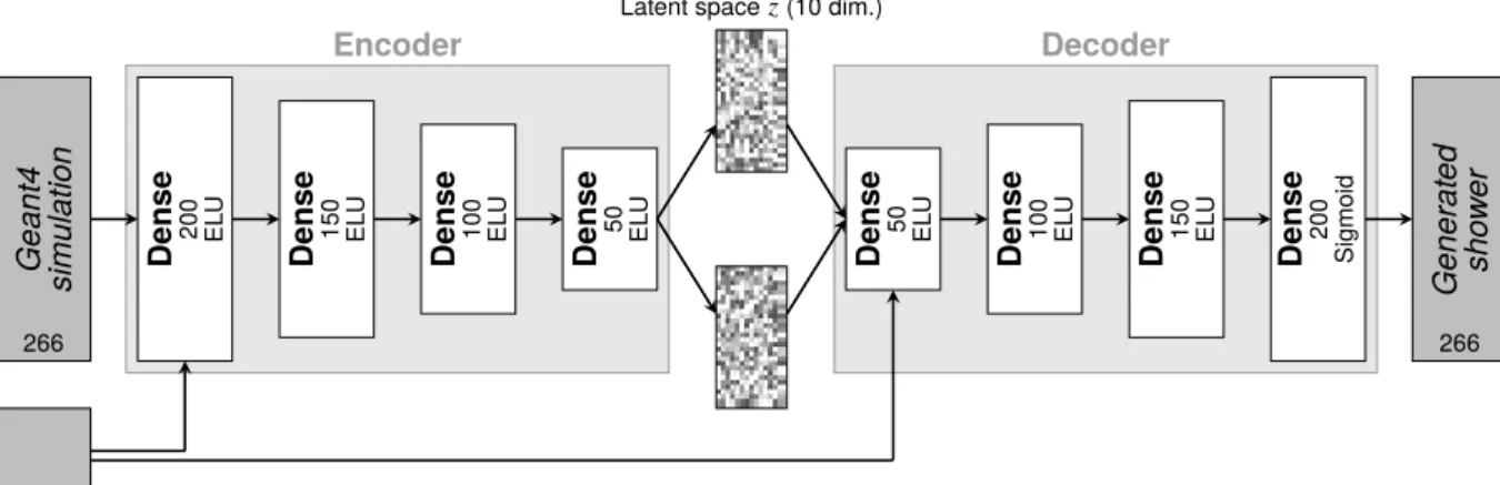
Encoder Latent spacez(10 dim.) Decoder Dense 50 EL U Dense 100 EL U Dense 150 EL U Dense 200 Sigmoid Gener at ed sho w er Dense 50 EL U Dense 100 EL U Dense 150 EL U Dense 200 EL U Geant4 simulation Particle energy 266 266
Figure 2: Schematic representation of the architecture of the VAE used in this note. It is composed of two stacked neural networks, each comprising of 4 hidden layers with decreasing/increasing number of units per layer, acting as encoder and decoder respectively. The model uses exponential linear units (ELUs) [22] and Sigmoid function for the output layer as activation functions. The implemented algorithm is conditioned on the energy of the incident particle to generate showers corresponding to a specific energy.
are selected. The dimension of the rectangle for the middle layer is chosen to be 7 × 7 cells in η × φ, containing more than 99 % of the total energy deposited by a typical shower in this layer. The dimensions of the remaining layers are chosen such that the spread in η and φ of the middle layer rectangle is covered. The dimensions for the presampler, front and back layer are 7 × 3, 56 × 3 and 4 × 7, respectively. In total the energy deposits in 266 cells are considered. For training the neural networks, the energy values are normalized to the energy of the incident particle.
All cells are selected with respect to the impact cell, defined as the cell in the middle layer closest to the extrapolated position of the photon, taking into account two possible alignments of the back layer and four possible alignments of the presampler and front layer with respect to the impact cell in the middle layer
when considering the simplified cuboid geometry. This is illustrated in Fig.1. Throughout the note, the
raw values of the calorimeter cells’ η and φ are used, i.e. not taking into account corrections accounting for imperfections of the detector, such as sagging under its own weight, or misalignment.
4 Algorithms
The architecture of the studied neural networks, the objective functions used in the training, as well as the tuning of the hyperparameters and their impact on the shower simulation are discussed in this section. A
general introduction to machine learning is given for example in Refs. [20,21].
4.1 Variational Autoencoders
VAEs [8, 9] are a class of unsupervised learning algorithms combining deep learning with variational
Bayesian methods and can be used as generative models. The algorithm explored in this note is composed of two stacked neural networks, each comprising of 4 hidden layers, acting as encoder and decoder
layers of the encoder and increases for the decoder. The implemented algorithm is conditioned [23,24] on the energy of the incident particle to generate showers corresponding to a specific energy. VAEs are latent
variable models [25] that introduce a set of random variables that are not directly observed but are used
to explain and reveal underlying structures in the data. As such, the encoder qθ(z|x) compresses the input
data x, i.e. energy deposits of a calorimeter shower, into a lower dimensional latent space z. It should
be noted explicitly that this latent representation is stochastic, i.e. qθ(z|x) maps x to a full distribution
rather than being a function x 7→ z. The decoder pφ(x|z) learns the inverse mapping, thus reconstructing
the original input from this latent representation. Once the model is trained, the decoder can be used independent of the encoder to generate new data ˜x, i.e. new calorimeter showers, by sampling z according to the prior probability density function p(z), which they are assumed to follow. As the prior a multivariate normal distribution with a covariance equal to the identity matrix is chosen.
The model is implemented in Keras 2.0.8 [26] using TensorFlow 1.3.0 [27] as the backend. The encoder
and decoder networks are connected and trained together with mini-batch gradient descent using Root
Mean Square Propagation (RMSProp) [28]. The training maximizes the variational lower bound on the
marginal log-likelihood for the data, approximated with reconstruction loss and the Kullback-Leibler
divergence [29]. The reconstruction loss Ez∼qθ(z |x)[log pφ(x|z)] penalizes the VAE for generating output
distributions different from the training data and thus characterizes the decoder’s capacity to recover data from the latent representation. Under the assumption that the reconstructed samples differ from the ground truth in a normal way, the mean-squared error (MSE) can be used to approximate the reconstruction loss. To synthesize new showers from the learned latent representation, the latent space is required to be continuous and must allow for smooth interpolations between the encoded instances. To ensure this, the
negative Kullback-Leibler divergence, measuring the divergence between qθ(z|x) and the prior probability
density function p(z), is included in the loss function. It is defined as
−KL(qθ(z|x)||p(z)) =
n
Õ
i=1
µ2i(xi) + σi2(xi) − log(σi(xi)) − 1 (1)
where µi and σi enter qφ(z/x) as the normal distribution N(z|µ, σ). Hence, the evidence lower bound,
i.e. the negative of the VAE loss, reads
log p(x) > Eqθ(z |x)[log pφ(x|z)] − KL(qθ(z|x)||p(z)). (2)
For fast calorimeter simulation, the objective function is augmented with additional terms related to the total energy deposition of a particle,
LEtot(x, ˜x) = k Õ i=1 xi− k Õ i=1 ˜xi (3) and the fraction of the energy deposited in each calorimeter layer,
LEi(x, ˜x) = ÍNi j=1xj Ík j=1xj − ÍNi j=1 ˜xj Ík j=1( ˜xj) (4)
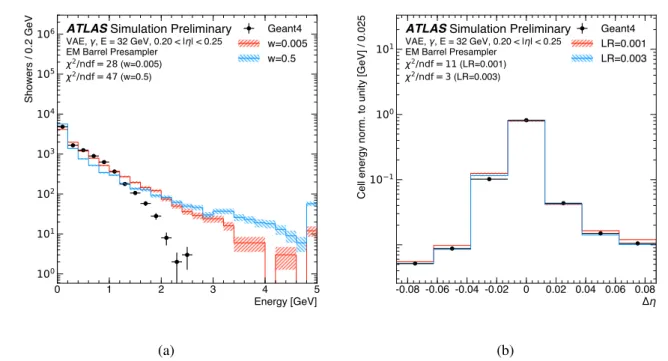
0 1 2 3 4 5 Energy [GeV] 100 101 102 103 104 105 106 Showers / 0.2 GeV
ATLAS Simulation Preliminary
VAE, γ, E = 32 GeV, 0.20 < |η| < 0.25 EM Barrel Presampler χ2/ndf = 28 (w=0.005) χ2/ndf = 47 (w=0.5) Geant4 w=0.005 w=0.5 (a) -0.08 -0.06 -0.04 -0.02 0 0.02 0.04 0.06 0.08 Δη 10−1 100 101
Cell energy norm. to unity [GeV] / 0.025
ATLAS Simulation Preliminary
VAE, γ, E = 32 GeV, 0.20 < |η| < 0.25 EM Barrel Presampler χ2/ndf = 11 (LR=0.001) χ2/ndf = 3 (LR=0.003) Geant4 LR=0.001 LR=0.003 (b)
Figure 3: (a) Comparison of the energy distribution in the presampler for different weights of the KL term. (b)Illustration of the impact of the learning rate on the energy weighted distance of the presampler cells in η from the impact point of the particle, weighted by the deposited energy, for an average shower. The comparisons are for photons with an energy of approximately 32 GeV in the range 0.20 < |η| < 0.25. The chosen bin width correspond to the cell width in the shown layer. The shown error bars and the hatched bands in both figures indicate the statistical uncertainty of the reference data and the synthesized samples, respectively. The underflow and overflow is included in the first and last bin of each distribution, respectively.
with the number of cells per shower shower, k, and the number of cells, Ni, in the i-th of M calorimeter
layer. The full loss function then is
LVAE(x, ˜x) = wrecoEz∼qθ(z |x)[log pφ(x|z)]−wKLKL(qθ(z|x)||p(z))+wEtotLEtot(x, ˜x)+ M
Õ
i
wiLEi(x, ˜x). (5)
Each term of the loss function is scaled by a weight, controlling the relative importance of the contributions during the optimization of the model. For example, the KL divergence acts as a regularization and changing its weight in the interval (0, 1] affects directly the generated distributions. The maximum value for the KL weight is 1, at which the loss becomes equivalent to the true variational lower bound,
see Eq. 2. The energy distribution in the presampler is shown in Fig. 3a for different weights of the
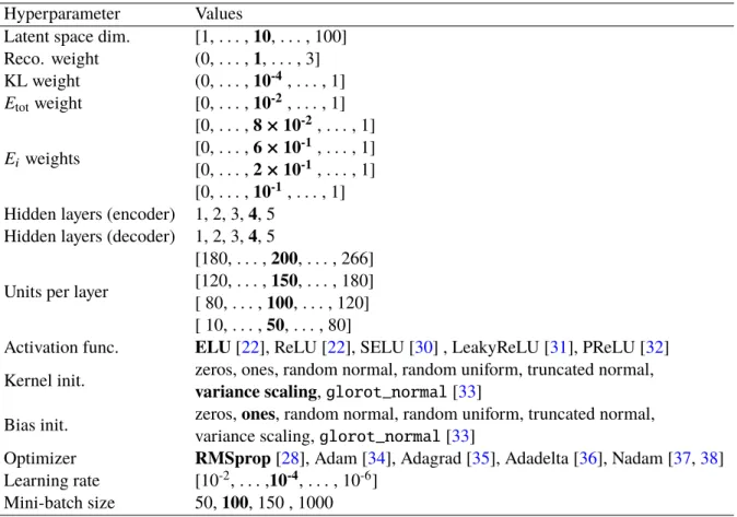
KL term. Additional hyperparameters of the model that require tuning are the depth of the encoder and decoder, the number of units in each layer of the neural networks, activation functions, bias and kernel initializers, the latent space dimension, the optimizer, its learning rate and the size of the mini-batches. Thus, minimizing the loss function evolves into a multi-objective optimization problem. The best set of hyperparameters is obtained from a grid search with cross validation, simultaneously minimizing the
Hyperparameter Values
Latent space dim. [1, . . . , 10, . . . , 100]
Reco. weight (0, . . . , 1, . . . , 3] KL weight (0, . . . , 10-4, . . . , 1] Etotweight [0, . . . , 10-2, . . . , 1] Eiweights [0, . . . , 8 × 10⁻², . . . , 1] [0, . . . , 6 × 10⁻¹, . . . , 1] [0, . . . , 2 × 10⁻¹, . . . , 1] [0, . . . , 10-1, . . . , 1]
Hidden layers (encoder) 1, 2, 3, 4, 5 Hidden layers (decoder) 1, 2, 3, 4, 5 Units per layer
[180, . . . , 200, . . . , 266] [120, . . . , 150, . . . , 180] [ 80, . . . , 100, . . . , 120] [ 10, . . . , 50, . . . , 80]
Activation func. ELU[22], ReLU [22], SELU [30] , LeakyReLU [31], PReLU [32]
Kernel init. zeros, ones, random normal, random uniform, truncated normal,
variance scaling, glorot_normal [33]
Bias init. zeros, ones, random normal, random uniform, truncated normal,variance scaling, glorot_normal [33]
Optimizer RMSprop[28], Adam [34], Adagrad [35], Adadelta [36], Nadam [37,38]
Learning rate [10-2, . . . ,10-4, . . . , 10-6]
Mini-batch size 50, 100, 150 , 1000
Table 1: Summary the results of the grid search performed to optimize the hyperparameters of the VAE for simulating calorimeter showers for photons. The optimal parameter is typeset in bold font.
Kolmogorov-Smirnov (KS) distance2between the synthesized showers and the Geant4 showers computed
for the total energy deposited in each layer. As an example, Fig.3billustrates the impact of the learning
rate on the shower generation. Larger learning rates increase the speed of the convergence of the model
at the cost of accuracy in the training phase, but results in a better generalization of the model. Table1
summarizes the results of the grid search performed to optimize the hyperparameters. The parameters with the largest effect on the quality of the synthesized showers are the weights in the loss function and the dimension of the latent space. The training of the VAE converges in 100 epochs within 2 min using the
full available training statistics on a Intel®Core™ i7-7500U Processor with a processor base frequency of
2.70 GHz and reading the training data from memory with a clock speed of 1867 MHz. Trainings for the hyperparameter optimization are performed in parallel on multiple CPUs. The last epoch of the training is used for synthesizing the presented showers.
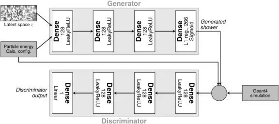
4.2 Generative Adversarial Networks
GANs are unsupervised learning algorithms implemented as a deep generative neural network taking
feedback from an additional discriminative neural network. Originally developed as a minimax game [39,
2The KS distance between two distributions is defined as the largest distance between the respective cumulative distribution functions.
Generator Discriminator Dense 128 LeakyR eL U Dense 128 LeakyR eL U Dense 128 LeakyR eL U Dense L1reg., 266 Sigmoid Particle energy Calo. config. Latent spacez Dense 1
Linear LeakyR 128 Dense
eL U Dense 128 LeakyR eL U Dense 128 LeakyR eL U Geant4 simulation Generated shower Discriminator output
Figure 4: Schematic representation of the architecture of the GAN used in this note. It is composed of two neural networks. The generator takes as input 300 random numbers drawn from the latent space distribution and is conditioned on the input particles’ energy as well as the alignments of the calorimeter cells. The discriminator compares synthesized showers from the generator to showers generated by Geant4. The model uses leaky rectified linear units (LeakyReLUs) [31] as activation functions for the hidden layers. The output layer of the generator and discriminator is using a Sigmoid and a linear function as activation function, respectively.
40] for generating realistic looking natural images [10], GANs have a wide range of applications including
calorimeter simulation [11–13]. The algorithm explored in this note is composed of two neural networks,
a generator and a discriminator. The model is conditioned on the energy of the incident particle and the
alignments the calorimeter cells in η and φ, discussed in Sec.3, as the model was found to be sensitive to
those. The detailed architecture of the two networks is illustrated in Fig.4.
The generator and discriminator networks are trained together with mini-batch gradient descent using
the Adam optimizer [34]. The generator network learns a mapping from a latent space distribution z to
the distribution of interest, i.e. energy deposits of a calorimeter shower. These shower candidates are compared to calorimeter showers from full simulation by the discriminator whose training objective is to identify the synthesized instances. The generator is trained to increase the discriminator’s misclassification rate and thus generate gradually more realistic distributions.
For a classification task commonly the binary cross entropy [41,42] between the true distribution and the
generated distribution is minimized. This corresponds to minimizing the negative log likelihood, which is equivalent to minimizing the KL divergence between the two distributions. However, the KL divergence does not encode an underlying metric on the data space, i.e. no notion of similarity. To introduce a
measure of the distance between the two distributions, the Wasserstein distance [43,44] between the true
and synthesized showers is used in the loss function instead [45,46]. This choice improves the stability
of the training, avoids mode collapse, provides a meaningful interpretation of the discriminator loss, and thus increases the quality of the generated showers.
The discriminator estimates a function that maximally separates the true and synthesized showers which
must lie in the space of 1-Lipschitz functions3 [43, 44]. The Lipschitz constraint is enforced through
3A real valued function f : R → R is called K-Lipschitz continuous if there exists a positive real constant K such that,
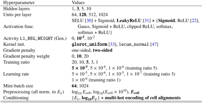
Hyperparameter Values
Hidden layers 1, 3, 5, 10
Units per layer 64, 128, 512, 1024
Activation func. SELU [Gauss, Sigmoid + ReLU, clipped ReLU, softmax,30] + Sigmoid, LeakyReLU [31] + {Sigmoid, ReLU [22], softmax + ReLU}
Activity L1_REG_WEIGHT (Gen.) 0, 10-5, 10-2
Kernel init. glorot_uniform[33], lecun_normal [47]
Gradient penalty one-sided, two-sided
Gradient penalty weight 0, 10, 20
Training ratio 20, 10, 5, 3, 1 Learning rate 5 × 10 -5, 5 × 10⁻⁶, 1 × 10⁻⁶(training ratio 5) 5 × 10⁻⁵, 5 × 10⁻⁶, 1 × 10⁻⁵, 1 × 10⁻⁷(training ratio 3) 1 × 10⁻⁶(training ratio 1) Mini-batch size 64, 1024
Preprocessing (all norm. to Eγ) log10Ecell, log10(Ecell× 1010), Ecell
Conditioning {Eγ, log10Eγ} + multi-hot encoding of cell alignments
Table 2: Summary the results of the grid search performed to optimize the hyperparameters of the GAN for simulating calorimeter showers for photons. The optimal parameter is typeset in bold font. In addition to the architectures summarized in the table, generators and discriminators with differing number of hidden layers and units per layer were tested.
employing a two-sided gradient penalty [45] for gradients greater than one. The loss of the discriminator
then reads
LGAN= E˜x∼pgen[D( ˜x)] −x∼pGeant4E [D(x)] + λ Eˆx∼p
ˆx[(||∆ˆxD( ˆx)||2− 1)
2]. (6)
The term E
˜x∼pgen[D( ˜x)] represents the discriminator’s ability to correctly identify synthesized showers,
while the term E
x∼pGeant4[D(x)] represents the discriminator’s ability to correctly identify showers from
Geant4. The last term in the loss function, λ E
ˆx∼pˆx[(||∆ˆxD( ˆx)||2− 1)
2], is the two-sided gradient penalty,
where ˆx is a random point on the straight line connecting a point from the real distribution pGeant4
and generated distribution pgen. The algorithm is further extended to estimate conditional probabilities,
leaving the evaluation of the gradient penalty over the showers unchanged. The model is implemented in
Keras 2.0.8 [26] using TensorFlow 1.3.0 [27] as the backend.
An L1 activity regularizer4 is applied to the final layer of the generator to encourage the generation of
sparse energy deposits. The training results of the GAN vary depending on the initial random number chosen to seed the optimization. Hence, when performing an optimization of the hyperparameters of the model, four GANs are trained with different random number seeds and their average performance is
compared to avoid picking up random fluctuations. As an example, Fig.5shows the average performance
of various activation functions of the output layer in the generator. Both sigmoid and normal activation 4The rectilinear distance between two points, also called L1 norm, is defined as the sum of the absolute differences of their
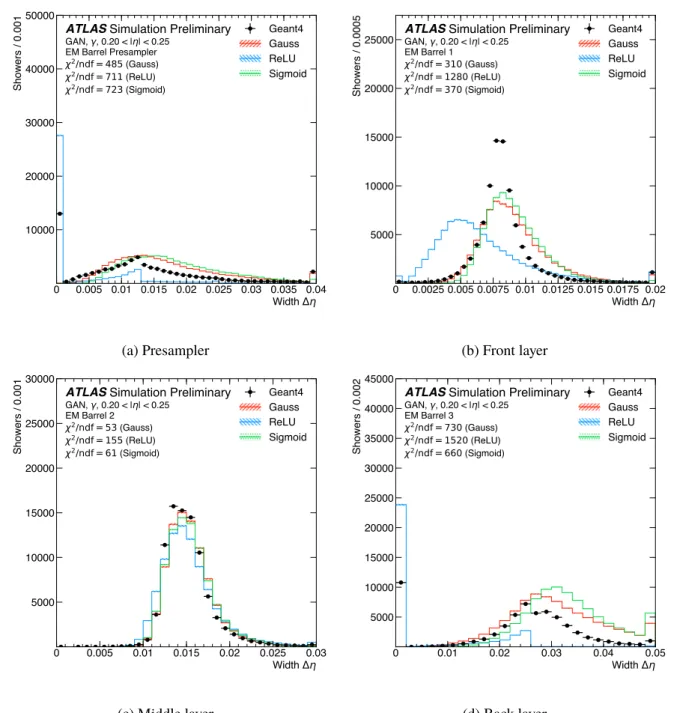
0 0.005 0.01 0.015 0.02 0.025 0.03 0.035 0.04 Width Δη 10000 20000 30000 40000 50000 Showers / 0.001
ATLAS Simulation Preliminary
GAN, γ, 0.20 < |η| < 0.25 EM Barrel Presampler χ2/ndf = 485 (Gauss) χ2/ndf = 711 (ReLU) χ2/ndf = 723 (Sigmoid) Geant4 Gauss ReLU Sigmoid (a) Presampler 0 0.0025 0.005 0.0075 0.01 0.0125 0.015 0.0175 0.02 Width Δη 5000 10000 15000 20000 25000 Showers / 0.0005
ATLAS Simulation Preliminary
GAN, γ, 0.20 < |η| < 0.25 EM Barrel 1 χ2/ndf = 310 (Gauss) χ2/ndf = 1280 (ReLU) χ2/ndf = 370 (Sigmoid) Geant4 Gauss ReLU Sigmoid (b) Front layer 0 0.005 0.01 0.015 0.02 0.025 0.03 Width Δη 5000 10000 15000 20000 25000 30000 Showers / 0.001
ATLAS Simulation Preliminary
GAN, γ, 0.20 < |η| < 0.25 EM Barrel 2 χ2/ndf = 53 (Gauss) χ2/ndf = 155 (ReLU) χ2/ndf = 61 (Sigmoid) Geant4 Gauss ReLU Sigmoid (c) Middle layer 0 0.01 0.02 0.03 0.04 0.05 Width Δη 5000 10000 15000 20000 25000 30000 35000 40000 45000 Showers / 0.002
ATLAS Simulation Preliminary
GAN, γ, 0.20 < |η| < 0.25 EM Barrel 3 χ2/ndf = 730 (Gauss) χ2/ndf = 1520 (ReLU) χ2/ndf = 660 (Sigmoid) Geant4 Gauss ReLU Sigmoid (d) Back layer
Figure 5: Average energy deposition in the cells of the individual calorimeter layers as a function of the distance in η from the impact point of the particles for photons in the range 0.20 < |η| < 0.25. The energy depositions from a full detector simulation (black markers) are shown as reference and compared to the ones exploiting three activation functions: sigmoid, Gauss, and ReLU. The shown error bars and the hatched bands indicate the statistical uncertainty of the reference data and the synthesized samples, respectively. The underflow and overflow is included in the first and last bin of each distribution, respectively.
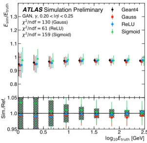
log10Etruth [GeV] 0.8 0.9 1 1.1 1.2 1.3 Esi m /Etr u th
ATLAS Simulation Preliminary
GAN, γ, 0.20 < |η| < 0.25 χ2/ndf = 130 (Gauss) χ2/ndf = 61 (ReLU) χ2/ndf = 159 (Sigmoid) Geant4 Gauss ReLU Sigmoid 0 0.5 1 1.5 2 2.5
log10Etruth [GeV]
0.95 1.0 1.05
Sim./Ref.
Figure 6: Energy response of the calorimeter as function of the true photon energy for particles in the range 0.20 < |η| < 0.25. The calorimeter response for the full detector simulation (black markers) is shown as reference and compared to the ones exploiting three activation functions: sigmoid, Gauss, and ReLU. The shown error bars indicate the resolution of the simulated energy deposits.
functions reproduce Geant4’s shower width in η better than a rectified linear unit activation (ReLU)
function [22]. While no significant impact of the choice on the energy resolution is found, the generated
mean energy shown in Fig. 6 shows a dependence on the choice of the activation function. Other
optimized hyperparameters include the number of layers in the neural networks and their width, the weight of the gradient penalty term, the weight of the L1 regularization, the number of training epochs, the learning rate and the size of the mini-batches used during the training. Furthermore, the choice between a one-sided or two sided gradient penalty is treated as a hyperparameter, too. Where possible, optimizations were performed one at a time, keeping other hyperparameter values at their default choice, but accounting for non-factorizable parameters when required. To select the optimal parameter values, the covariance matrix for the 266 cells is evaluated and compared to the full simulation. The same metric is used to select among the random seeds. For hyperparameter choices aiming at improving specific characteristics of the generated showers, distributions reflecting those are compared directly to Geant4, e.g. the successive application of Sigmoid and ReLU activation functions is expected to induce sparse showers. The parameters with the largest effect on the quality of the synthesized showers are
the choice of the activation functions and the conditioning. Table2 summarizes the results of the grid
search performed to optimize the hyperparameters. The training of the GAN, that is the discriminator and generator networks, converges in 50000 epochs within 7 h using approximately 5 % of the available
training statistics on a NVIDIA® Kepler™ GK210 GPU with a processing power of 2496 cores, each
clocked at 562 MHz. The card has a video RAM size of 12 GB with a clock speed of 5 GHz. The training data is read from memory. Trainings for the hyperparameter optimization are performed in parallel on multiple GPUs. It is expected to increase the number of showers used for the training while decreasing training times when fully utilising the distributed training capabilities and optimizing the data processing pipeline. The last epoch of the training is used for synthesizing the presented showers. Epoch-picking will be investigated in the future to cope with epoch-to-epoch fluctuations.
5 Results
To assess the quality of the generative models described in this note, synthesized calorimeter showers for single photons with varying energy are compared to the full detector simulation. Due to the stochastic nature of the shower development in the calorimeter, no individual shower can be compared. Instead, significant distributions used during the event reconstruction and particle identification, such as the total energy, the energy deposited in each calorimeter layer, and the relative distribution of energies in the calorimeter cells, are compared.
The algorithms presented in this note are designed to reproduce the calorimeter response to a specific particle and energy as the full detector simulation. Neither algorithm is taught about energy conservation explicitly, i.e. the sum of simulated energies may exceed the truth particle energy. The energy deposited
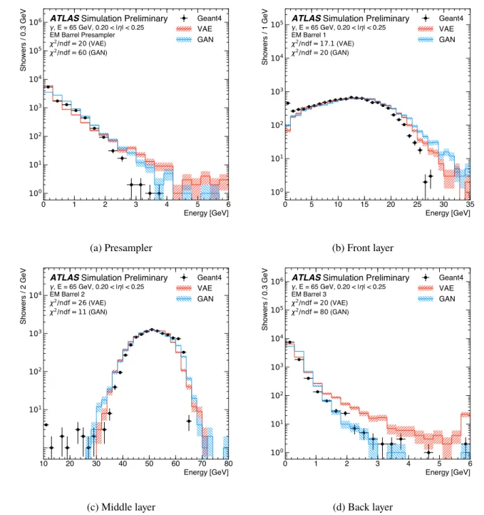
in the individual calorimeter layers is shown in Fig.7for photons with an energy of approximately 65 GeV
in the range 0.20 < |η| < 0.25,
Ei =
Õ
j∈cells
Ei j. (7)
Both VAE and GAN accurately describe the bulk of the energy deposits in the individual calorimeter layers. However, the agreement in the tails of the distributions is reduced and the generative models simulate showers with larger energies. This behavior indicates smaller correlations between the energies deposited in the layers for the synthesized showers as compared to Geant4.
The mean shower shape measured inside the calorimeter layers depends strongly on the longitudinal shower profile in the calorimeter and is used for example to distinguish photons from electrons. The
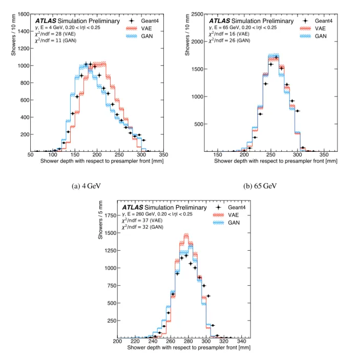
modeling of the longitudinal shower development is shown in Fig.8for photons with different energies in
the range 0.20 < |η| < 0.25. The reconstructed longitudinal shower center, in the following referred to as
shower depth, is calculated from the energy weighted mean of the longitudinal center positions dlayer of
all calorimeter layers,
d = E1 Õ
i∈layers
Eidi. (8)
Both VAE and GAN reproduce the shape of shower depth simulated by Geant4, but the distributions computed from the synthesized showers are shifted with respect to the Geant4 ones, in particular for lower energetic particles. This effect is explained by the mismodeling of the correlations between the energy deposits in the various calorimeter layers and the challenges posed by layers with low (and sparse) energy
deposits, i.e. showers starting not at the surface of the calorimeter, for example in Fig.7b.
Figure9shows the total energy response of the calorimeter to photons with an energy of approximately
65 GeV in the range 0.20 < |η| < 0.25,
E = Õ
i∈layers
Õ
j∈cells
Ei j. (9)
Figure10shows the simulated energy as a function of true photon energy. Both VAE and GAN reproduce
the mean shower energy simulated by Geant4. The modeling of the total energy response reflects the modeling of the underlying distributions, i.e. the energy deposited in the calorimeter layers, and enhances the mismodeling of the tails due to underestimating the underlying correlations observed in these. Both generative models simulate a wider spread of energies than Geant4. The GAN reproduces better the correlations between the energy deposits in the different layers, and therefore shows a smaller spread then the VAE.
0 1 2 3 4 5 6 Energy [GeV] 100 101 102 103 104 105 106 Showers / 0.3 GeV
ATLAS Simulation Preliminary
γ, E = 65 GeV, 0.20 < |η| < 0.25 EM Barrel Presampler χ2/ndf = 20 (VAE) χ2/ndf = 60 (GAN) Geant4 VAE GAN (a) Presampler 0 5 10 15 20 25 30 35 Energy [GeV] 100 101 102 103 104 105 Showers / 1 GeV
ATLAS Simulation Preliminary
γ, E = 65 GeV, 0.20 < |η| < 0.25 EM Barrel 1 χ2/ndf = 17.1 (VAE) χ2/ndf = 20 (GAN) Geant4 VAE GAN (b) Front layer 10 20 30 40 50 60 70 80 Energy [GeV] 101 102 103 104 Showers / 2 GeV
ATLAS Simulation Preliminary
γ, E = 65 GeV, 0.20 < |η| < 0.25 EM Barrel 2 χ2/ndf = 26 (VAE) χ2/ndf = 11 (GAN) Geant4 VAE GAN (c) Middle layer 0 1 2 3 4 5 6 Energy [GeV] 100 101 102 103 104 105 106 Showers / 0.3 GeV
ATLAS Simulation Preliminary
γ, E = 65 GeV, 0.20 < |η| < 0.25 EM Barrel 3 χ2/ndf = 20 (VAE) χ2/ndf = 80 (GAN) Geant4 VAE GAN (d) Back layer
Figure 7: Energy deposited in the individual calorimeter layers for photons with an energy of approximately 65 GeV in the range 0.20 < |η| < 0.25. The energy depositions from a full detector simulation (black markers) are shown as reference and compared to the ones of a VAE (solid red line) and a GAN (solid blue line). The shown error bars and the hatched bands indicate the statistical uncertainty of the reference data and the synthesized samples, respectively. The underflow and overflow is included in the first and last bin of each distribution, respectively.
50 100 150 200 250 300 350 Shower depth with respect to presampler front [mm] 200 400 600 800 1000 1200 1400 1600 Showers / 10 mm
ATLAS Simulation Preliminary
γ, E = 4 GeV, 0.20 < |η| < 0.25 χ2/ndf = 28 (VAE) χ2/ndf = 11 (GAN) Geant4 VAE GAN (a) 4 GeV 150 200 250 300 350
Shower depth with respect to presampler front [mm] 500 1000 1500 2000 2500 Showers / 10 mm
ATLAS Simulation Preliminary
γ, E = 65 GeV, 0.20 < |η| < 0.25 χ2/ndf = 16 (VAE) χ2/ndf = 26 (GAN) Geant4 VAE GAN (b) 65 GeV 200 220 240 260 280 300 320 340
Shower depth with respect to presampler front [mm] 250 500 750 1000 1250 1500 1750 Showers / 5 mm
ATLAS Simulation Preliminary
γ, E = 260 GeV, 0.20 < |η| < 0.25 χ2/ndf = 37 (VAE) χ2/ndf = 32 (GAN) Geant4 VAE GAN (c) 260 GeV
Figure 8: Reconstructed longitudinal shower center for photons with an energy of(a)4 GeV,(b)65 GeV and(c) 260 GeV in the range 0.20 < |η| < 0.25. The shower depth for the full detector simulation (black markers) is shown as reference and compared to the ones of a VAE (solid red line) and a GAN (solid blue line). The shown error bars and the hatched bands indicate the statistical uncertainty of the reference data and the synthesized samples, respectively. The underflow and overflow is included in the first and last bin of each distribution, respectively.
40 50 60 70 80 90 Shower energy [GeV]
101 102 103 104 105 106 107 Showers / 1 GeV
ATLAS Simulation Preliminary
γ, E = 65 GeV, 0.20 < |η| < 0.25 χ2/ndf = 267 (VAE) χ2/ndf = 235 (GAN) Geant4 VAE GAN
Figure 9: Total energy response of the calorimeter to photons with an energy of approximately 65 GeV in the range 0.20 < |η| < 0.25. The calorimeter response for the full detector simulation (black markers) is shown as reference and compared to the ones of a VAE (solid red line) and a GAN (solid blue line). The shown error bars and the hatched bands indicate the statistical uncertainty of the reference data and the synthesized samples, respectively. The underflow and overflow is included in the first and last bin of each distribution, respectively.
log10Etruth [GeV]
0.8 0.9 1 1.1 1.2 1.3 Esim /Etr u th
ATLAS Simulation Preliminary
γ, 0.20 < |η| < 0.25 χ2/ndf = 400 (VAE) χ2/ndf = 130 (GAN) Geant4 VAE GAN 0 0.5 1 1.5 2 2.5
log10Etruth [GeV]
0.95 1.0 1.05
Sim./Ref.
Figure 10: Energy response of the calorimeter as function of the true photon energy for particles in the range 0.20 < |η| < 0.25. The calorimeter response for the full detector simulation (black markers) is shown as reference and compared to the ones of a VAE (red markers) and a GAN (blue markers). The shown error bars indicate the resolution of the simulated energy deposits.
Figures11and12show the average energy deposition in the cells of the individual calorimeter layers as a function of the distance in η and φ from the impact point of the particles for photons with an energy of approximately 65 GeV in the range 0.20 < |η| < 0.25. The distances ∆η and ∆φ are calculated from the center of the cell as the energy distribution within one calorimeter cell is not known. To further probe the modeling of the average lateral shower shapes of the synthesized showers, the energy weighted mean and
width of the ∆η and ∆φ distributions for the middle layer are compared to the full simulation in Figs.13
and14 respectively. Both VAE and GAN reproduce the reference average lateral shower shape within
a precision of approximately 20 to 40 % with differences increasing with the distance from the shower center. A wider spread in energy weighted width of the ∆η and ∆φ distributions is observed for both generative models. These effects are driven by the increasing sparsity of the showers towards the edges and hence the deviation of individual shower shapes from the average shower shape, i.e. an effect that the algorithms have not been optimized for explicitly.
-0.08 -0.06 -0.04 -0.02 0 0.02 0.04 0.06 0.08 Δη
10−1
100
101
Cell energy norm. to unity [GeV] / 0.025
ATLAS Simulation Preliminary
γ, E = 65 GeV, 0.20 < |η| < 0.25 EM Barrel Presampler χ2/ndf = 60 (VAE) χ2/ndf = 110 (GAN) Geant4 VAE GAN (a) Presampler -0.08 -0.06 -0.04 -0.02 0 0.02 0.04 0.06 0.08 Δη 10−3 10−2 10−1 100
Cell energy norm. to unity [GeV] / 0.0031
ATLAS Simulation Preliminary
γ, E = 65 GeV, 0.20 < |η| < 0.25 EM Barrel 1 χ2/ndf = 40 (VAE) χ2/ndf = 300 (GAN) Geant4 VAE GAN (b) Front layer -0.08 -0.06 -0.04 -0.02 0 0.02 0.04 0.06 0.08 Δη 10−1 100 101
Cell energy norm. to unity [GeV] / 0.025
ATLAS Simulation Preliminary
γ, E = 65 GeV, 0.20 < |η| < 0.25 EM Barrel 2 χ2/ndf = 50 (VAE) χ2/ndf = 270 (GAN) Geant4 VAE GAN (c) Middle layer -0.1 -0.075 -0.05 -0.025 0 0.025 0.05 0.075 0.1 Δη 100 101
Cell energy norm. to unity [GeV] / 0.05
ATLAS Simulation Preliminary
γ, E = 65 GeV, 0.20 < |η| < 0.25 EM Barrel 3 χ2/ndf = 160 (VAE) χ2/ndf = 30 (GAN) Geant4 VAE GAN (d) Back layer
Figure 11: Average energy deposition in the cells of the individual calorimeter layers as a function of the distance in η from the impact point of the particles for photons with an energy of approximately 65 GeV in the range 0.20 < |η| < 0.25. The chosen bin widths correspond to the cell widths in each of the layers. The energy depositions from a full detector simulation (black markers) are shown as reference and compared to the ones of a VAE (solid red line) and a GAN (solid blue line). The shown error bars and the hatched bands indicate the statistical uncertainty of the reference data and the synthesized samples, respectively. The underflow and overflow is included in the first and last bin of each distribution, respectively. The showers simulated by Geant4 deposit on average approximately 0.7 %, 17.2 %, 79.3 % and 0.4 % of the true photon energy in the presampler, front, middle and back layer, respectively. The showers synthesized by the VAE (GAN) deposit on average approximately 0.6 % (0.8 %), 19.1 % (19.8 %), 77.6 % (78.1 %) and 0.6 % (0.5 %) of the true photon energy in the presampler, front, middle and back layer, respectively.
-0.1 -0.05 0 0.05 0.1 Δϕ [rad]
100
101
Cell energy norm. to unity [GeV] / 0.0982 rad
ATLAS Simulation Preliminary
γ, E = 65 GeV, 0.20 < |η| < 0.25 EM Barrel Presampler χ2/ndf = 107 (VAE) χ2/ndf = 83 (GAN) Geant4 VAE GAN (a) Presampler -0.1 -0.05 0 0.05 0.1 Δϕ [rad] 100 101
Cell energy norm. to unity [GeV] / 0.0982 rad
ATLAS Simulation Preliminary
γ, E = 65 GeV, 0.20 < |η| < 0.25 EM Barrel 1 χ2/ndf = 143 (VAE) χ2/ndf = 108 (GAN) Geant4 VAE GAN (b) Front layer -0.08 -0.06 -0.04 -0.02 0 0.02 0.04 0.06 0.08 Δϕ [rad] 10−1 100 101
Cell energy norm. to unity [GeV] / 0.0245 rad
ATLAS Simulation Preliminary
γ, E = 65 GeV, 0.20 < |η| < 0.25 EM Barrel 2 χ2/ndf = 20 (VAE) χ2/ndf = 300 (GAN) Geant4 VAE GAN (c) Middle layer -0.08 -0.06 -0.04 -0.02 0 0.02 0.04 0.06 0.08 Δϕ [rad] 10−1 100 101
Cell energy norm. to unity [GeV] / 0.0245 rad
ATLAS Simulation Preliminary
γ, E = 65 GeV, 0.20 < |η| < 0.25 EM Barrel 3 χ2/ndf = 160 (VAE) χ2/ndf = 30 (GAN) Geant4 VAE GAN (d) Back layer
Figure 12: Average energy deposition in the cells of the individual calorimeter layers as a function of the distance in φ from the impact point of the particles for photons with an energy of approximately 65 GeV in the range 0.20 < |η| < 0.25. The chosen bin widths correspond to the cell widths in each of the layers. The energy depositions from a full detector simulation (black markers) are shown as reference and compared to the ones of a VAE (solid red line) and a GAN (solid blue line). The shown error bars and the hatched bands indicate the statistical uncertainty of the reference data and the synthesized samples, respectively. The underflow and overflow is included in the first and last bin of each distribution, respectively. The showers simulated by Geant4 deposit on average approximately 0.7 %, 17.2 %, 79.3 % and 0.4 % of the true photon energy in the presampler, front, middle and back layer, respectively. The showers synthesized by the VAE (GAN) deposit on average approximately 0.6 % (0.8 %), 19.1 % (19.8 %), 77.6 % (78.1 %) and 0.6 % (0.5 %) of the true photon energy in the presampler, front, middle and back layer, respectively.
-0.02 -0.01 0 0.01 0.02 Mean Δη 102 103 104 105 106 Showers / 0.002
ATLAS Simulation Preliminary
γ, E = 65 GeV, 0.20 < |η| < 0.25 EM Barrel 2 χ2/ndf = 14 (VAE) χ2/ndf = 9 (GAN) Geant4 VAE GAN (a) 0.005 0.01 0.015 0.02 0.025 0.03 Width Δη 101 102 103 104 105 106 Showers / 0.001
ATLAS Simulation Preliminary
γ, E = 65 GeV, 0.20 < |η| < 0.25 EM Barrel 2 χ2/ndf = 90 (VAE) χ2/ndf = 150 (GAN) Geant4 VAE GAN (b)
Figure 13: Energy weighted(a)mean and(b)width of the ∆η distribution for the middle layer for photons with an energy of approximately 65 GeV in the range 0.20 < |η| < 0.25. The distributions from a full detector simulation (black markers) are shown as reference and compared to the ones of a VAE (solid red line) and a GAN (solid blue line). The shown error bars and the hatched bands indicate the statistical uncertainty of the reference data and the synthesized samples, respectively. The underflow and overflow is included in the first and last bin of each distribution, respectively.
-0.02 -0.01 0 0.01 0.02 Mean Δϕ [rad] 103 104 105 106 107 Showers / 0.002 rad
ATLAS Simulation Preliminary
γ, E = 65 GeV, 0.20 < |η| < 0.25 EM Barrel 2 χ2/ndf = 19 (VAE) χ2/ndf = 7 (GAN) Geant4 VAE GAN (a) 0.005 0.01 0.015 0.02 0.025 0.03 Width Δϕ [rad] 101 102 103 104 105 106 107 Showers / 0.001 rad
ATLAS Simulation Preliminary
γ, E = 65 GeV, 0.20 < |η| < 0.25 EM Barrel 2 χ2/ndf = 130 (VAE) χ2/ndf = 220 (GAN) Geant4 VAE GAN (b)
Figure 14: Energy weighted(a)mean and(b)width of the ∆φ distribution for the middle layer for photons with an energy of approximately 65 GeV in the range 0.20 < |η| < 0.25. The distributions from a full detector simulation (black markers) are shown as reference and compared to the ones of a VAE (solid red line) and a GAN (solid blue line). The shown error bars and the hatched bands indicate the statistical uncertainty of the reference data and the synthesized samples, respectively. The underflow and overflow is included in the first and last bin of each distribution, respectively.
6 Conclusion
This note presents the first application of generative models for simulating particle showers in the ATLAS calorimeter. Two algorithms, a VAE and a GAN, have been used to learn the response of the EM calorimeter for photons with energies between approximately 1 and 260 GeV in the range 0.20 < |η| < 0.25. The properties of synthesized showers show promising agreement with showers from a full detector simulation using Geant4, demonstrating the feasibility of using such algorithms for fast calorimeter simulation for the ATLAS experiment in the future and opening the possibility to complement current techniques. In addition to conditioning the algorithms on different particle types and incorporating other regions of the calorimeter, further studies are needed to achieve the required accuracy for employing the algorithms for physics analyses.
Acknowledgement
We would like to thank Gilles Louppe (Université de Liège) for valuable discussions.
References
[1] ATLAS Collaboration, The ATLAS Experiment at the CERN Large Hadron Collider,
JINST 3 (2008) S08003.
[2] L. Evans and P. Bryant, LHC Machine,JINST 3 (2008) S08001, ed. by L. Evans.
[3] S. Agostinelli et al., GEANT4: A Simulation toolkit,Nucl.Instrum.Meth. A506 (2003) 250.
[4] ATLAS Collaboration, The ATLAS Simulation Infrastructure,Eur. Phys. J. C 70 (2010) 823,
arXiv:1005.4568 [physics.ins-det].
[5] ATLAS Collaboration,
The simulation principle and performance of the ATLAS fast calorimeter simulation FastCaloSim,
ATL-PHYS-PUB-2010-013, 2010, url:https://cds.cern.ch/record/1300517.
[6] F. Dias, The new ATLAS Fast Calorimeter Simulation, PoS ICHEP2016 (2016) 184. [7] J. Schaarschmidt, The new ATLAS Fast Calorimeter Simulation,
J. Phys. Conf. Ser. 898 (2017) 042006.
[8] D. P. Kingma and M. Welling, Auto-Encoding Variational Bayes, ArXiv e-prints (2013),
arXiv:1312.6114 [stat.ML].
[9] D. Jimenez Rezende, S. Mohamed and D. Wierstra,
Stochastic Backpropagation and Approximate Inference in Deep Generative Models,
ArXiv e-prints (2014), arXiv:1401.4082 [stat.ML].
[10] I. J. Goodfellow et al., Generative Adversarial Networks, ArXiv e-prints (2014),
arXiv:1406.2661 [stat.ML].
[11] L. de Oliveira, M. Paganini and B. Nachman, Learning Particle Physics by Example:
Location-Aware Generative Adversarial Networks for Physics Synthesis, Comput. Softw. Big Sci. 1 (2017) 4, arXiv:1701.05927 [stat.ML].
[12] M. Paganini, L. de Oliveira and B. Nachman, Accelerating Science with Generative Adversarial
Networks: An Application to 3D Particle Showers in Multilayer Calorimeters, Phys. Rev. Lett. 120 (2018) 042003, arXiv:1705.02355 [hep-ex].
[13] M. Paganini, L. de Oliveira and B. Nachman, CaloGAN : Simulating 3D high energy particle
showers in multilayer electromagnetic calorimeters with generative adversarial networks, Phys. Rev. D97 (2018) 014021, arXiv:1712.10321 [hep-ex].
[14] J. Allison et al., Recent developments in Geant4,Nucl. Instrum. Meth. A835 (2016) 186.
[15] M. P. Guthrie, R. G. Alsmiller and H. W. Bertini, Calculation of the capture of negative pions in
light elements and comparison with experiments pertaining to cancer radiotherapy, Nucl. Instrum. Meth. 66 (1968) 29.
[16] H. W. Bertini,
Intranuclear-cascade calculation of the secondary nucleon spectra from nucleon-nucleus interactions in the energy range 340 to 2900 mev and comparisons with experiment, Phys. Rev. 188 (1969) 1711.
[17] H. W. Bertini and M. P. Guthrie,
News item results from medium-energy intranuclear-cascade calculation, Nucl. Phys. A169 (1971) 670.
[18] B. Andersson, G. Gustafson and B. Nilsson-Almqvist, A Model for Low p(t) Hadronic Reactions,
with Generalizations to Hadron - Nucleus and Nucleus-Nucleus Collisions, Nucl. Phys. B281 (1987) 289.
[19] B. Nilsson-Almqvist and E. Stenlund,
Interactions Between Hadrons and Nuclei: The Lund Monte Carlo, Fritiof Version 1.6, Comput. Phys. Commun. 43 (1987) 387.
[20] C. M. Bishop, Pattern Recognition and Machine Learning, Springer, 2006, isbn: 978-0-387-31073-2.
[21] T. Hastie, R. Tibshirani and J. Friedman, The Elements of Statistical Learning, 2nd ed., Springer, 2009, isbn: 978-0-387-84857-0.
[22] D. Clevert, T. Unterthiner and S. Hochreiter,
Fast and Accurate Deep Network Learning by Exponential Linear Units (ELUs), (2015),
arXiv:1511.07289.
[23] K. Sohn, H. Lee and X. Yan,
“Learning Structured Output Representation using Deep Conditional Generative Models”,
Advances in Neural Information Processing Systems 28,
ed. by C. Cortes, N. D. Lawrence, D. D. Lee, M. Sugiyama and R. Garnett, Curran Associates, Inc., 2015 3483,
url: http://papers.nips.cc/paper/5775-learning-structured-output-representation-using-deep-conditional-generative-models.pdf.
[24] J. Walker, C. Doersch, A. Gupta and M. Hebert,
An Uncertain Future: Forecasting from Static Images using Variational Autoencoders,
ArXiv e-prints (2016), arXiv:1606.07873 [cs.CV].
[25] C. Spearman, "General Intelligence," Objectively Determined and Measured, The American Journal of Psychology 15 (1904) 201.
[26] F. Chollet et al., Keras, 2015, url:https://keras.io.
[27] Martín Abadi et al., TensorFlow: Large-Scale Machine Learning on Heterogeneous Systems,
2015, url:https://www.tensorflow.org/.
[28] T. Tieleman and G. Hinton,
Lecture 6.5 – RMSProp: Divide the gradient by a running average of its recent magnitude,
Coursera: Neural networks for machine learning 4 (2012) 26.
[29] S. Kullback and R. A. Leibler, On Information and Sufficiency,Ann. Math. Statist. 22 (1951) 79,
url:https://doi.org/10.1214/aoms/1177729694.
[30] G. Klambauer, T. Unterthiner, A. Mayr and S. Hochreiter, Self-Normalizing Neural Networks,
(2017), arXiv:1706.02515.
[31] A. L. Maas, A. Y. Hannun and A. Y. Ng,
“Rectifier nonlinearities improve neural network acoustic models”,
in ICML Workshop on Deep Learning for Audio, Speech and Language Processing, 2013.
[32] K. He, X. Zhang, S. Ren and J. Sun,
Delving Deep into Rectifiers: Surpassing Human-Level Performance on ImageNet Classification,
(2015), arXiv:1502.01852.
[33] X. Glorot and Y. Bengio,
“Understanding the difficulty of training deep feedforward neural networks”,
Proceedings of the Thirteenth International Conference on Artificial Intelligence and Statistics,
ed. by Y. W. Teh and M. Titterington, vol. 9, Proceedings of Machine Learning Research,
PMLR, 2010 249, url:http://proceedings.mlr.press/v9/glorot10a.html.
[34] D. P. Kingma and J. Ba, Adam: A Method for Stochastic Optimization, ArXiv e-prints (2014),
arXiv:1412.6980 [cs.LG].
[35] J. Duchi, E. Hazan and Y. Singer,
Adaptive Subgradient Methods for Online Learning and Stochastic Optimization,
J. Mach. Learn. Res. 12 (2011) 2121, issn: 1532-4435,
url:http://dl.acm.org/citation.cfm?id=1953048.2021068.
[36] M. D. Zeiler, ADADELTA: An Adaptive Learning Rate Method, (2012), arXiv:1212.5701.
[37] I. Sutskever, J. Martens, G. Dahl and G. Hinton,
“On the importance of initialization and momentum in deep learning”,
Proceedings of the 30th International Conference on Machine Learning,
ed. by S. Dasgupta and D. McAllester, vol. 28, Proceedings of Machine Learning Research 3,
PMLR, 2013 1139, url:http://proceedings.mlr.press/v28/sutskever13.html.
[38] T. Dozat, “Incorporating Nesterov Momentum into Adam”, 2015. [39] J. von Neumann, Sur la theéorie des jeux,
Comptes Rendus de l’Académie des Sciences 186.25 (1928) 1689.
[40] J. von Neumann, Zur Theorie der Gesellschaftsspiele., Mathematische Annalen 100 (1928) 295. [41] R. Y. Rubinstein and D. P. Kroese, The Cross Entropy Method: A Unified Approach To
Combinatorial Optimization, Monte-carlo Simulation (Information Science and Statistics),
[42] P.-T. de Boer, D. P. Kroese, S. Mannor and R. Y. Rubinstein,
A Tutorial on the Cross-Entropy Method,Annals of Operations Research 134 (2005) 19,
issn: 1572-9338, url:https://doi.org/10.1007/s10479-005-5724-z.
[43] F. L. Hitchcock, The Distribution of a Product from Several Sources to Numerous Localities,
Journal of Mathematics and Physics 20 (1941) 224. [44] L. Vaserstein,
Markovian processes on countable space product describing large systems of automata., Russian,
Probl. Peredachi Inf. 5 (1969) 64, issn: 0555-2923.
[45] I. Gulrajani, F. Ahmed, M. Arjovsky, V. Dumoulin and A. C. Courville,
Improved Training of Wasserstein GANs, (2017), arXiv:1704.00028.
[46] M. Arjovsky, S. Chintala and L. Bottou, Wasserstein GAN, ArXiv e-prints (2017),
arXiv:1701.07875 [stat.ML].
[47] Y. LeCun, L. Bottou, G. B. Orr and K.-R. Müller, “Efficient BackProp”,
Neural Networks: Tricks of the Trade, ed. by G. B. Orr and K.-R. Müller, Springer, 1998 9,