HAL Id: hal-01819519
https://hal.insa-toulouse.fr/hal-01819519
Submitted on 3 Dec 2018HAL is a multi-disciplinary open access archive for the deposit and dissemination of sci-entific research documents, whether they are pub-lished or not. The documents may come from teaching and research institutions in France or abroad, or from public or private research centers.
L’archive ouverte pluridisciplinaire HAL, est destinée au dépôt et à la diffusion de documents scientifiques de niveau recherche, publiés ou non, émanant des établissements d’enseignement et de recherche français ou étrangers, des laboratoires publics ou privés.
Stability of ball-end milling on warped surface:
semi-analytical and experimental analysis
Oleksii Shtehin, Vincent Wagner, Sébastien Seguy, Yann Landon, Gilles
Dessein, Michel Mousseigne
To cite this version:
Oleksii Shtehin, Vincent Wagner, Sébastien Seguy, Yann Landon, Gilles Dessein, et al.. Stability of ball-end milling on warped surface: semi-analytical and experimental analysis. International Journal of Advanced Manufacturing Technology, Springer Verlag, 2017, 89 (9-12), pp.2557-2569. �10.1007/s00170-016-9656-3�. �hal-01819519�
Stability of ball end milling on warped surface: semi-analytical and
experimental analysis
OO. Shtehina, V. Wagnerb, S. Seguyc, Y. Landonc, G. Desseinb, M. Mousseignec
aZhytomyr State Technological University, Chernyakhovsky street 103, Zhytomyr, Ukraine,
10005
bLaboratoire Génie de Production, ENIT-INPT, Université de Toulouse, Tarbes, France cUniversité de Toulouse, Institut Clément Ader (ICA), CNRS-INSA-ISAE-Mines Albi-UPS,
Toulouse, France
OO. SHTEHIN shtegin@gmail.com V. WAGNER vincent.wagner@enit.fr S. SEGUY sebastien.seguy@insa-toulouse.fr Y. LANDON yann.landon@univ-tlse3.fr G. DESSEIN gilles.dessein@enit.fr M. MOUSSEIGNE michel.mousseigne@univ-tlse3.fr Abstract
This paper presents a study of warped surfaces machining with ball end milling. A specific model based on the classical stability lobe theory was used and improved with important aspects. The non-linear effect of radial allowance on the contact angle was integrated by an original averaging method. The cutting coefficients are updated in order to follow effective radius and cutting velocity. An original experimental procedure was developed in order to compute the cutting coefficient for various inclined surfaces. More complete experimental analysis was conducted in order to study the effect of machining parameters on the stability of inclined surface milling. The comparison between experiment and simulation shows good correlation for the prediction of stable cutting condition.
Stability of ball end milling on warped surface: semi-analytical and
experimental analysis
Abstract
This paper presents a study of warped surfaces machining with ball end milling. A specific model based on the classical stability lobe theory was used and improved with important aspects. The non-linear effect of radial allowance on the contact angle was integrated by an original averaging method. The cutting coefficients are updated in order to follow effective radius and cutting velocity. An original experimental procedure was developed in order to compute the cutting coefficient for various inclined surfaces. More complete experimental analysis was conducted in order to study the effect of machining parameters on the stability of inclined surface milling. The comparison between experiment and simulation shows good correlation for the prediction of stable cutting condition.
1. Introduction
High-performance machining of crooked spatial surfaces is a complex task, which solution are supremely important for various type of industry like casting, molding, dies production and monolithic components in the aeronautical industry. In most cases, finishing of such surfaces is carried out with ball end mills on CNC machines. Ball end milling of inclined surfaces can be considered as particular case of crooked spatial surfaces machining. This process is widely used, which is caused by competitive prices of machines and accessories and by the wide spectrum of the problems that can be solved with this machining process. However, the main limitation of this machining method consists in difficulty of tilt and lead angles control. Dynamical properties of ball end milling process are specific and its dynamic behaviour prediction is a knotty question. Particularly, it concerns ensuring process stability. Chatter vibrations are relevant for all types of cutting. Their genesis consists in regenerative effect. One of the first studies about chatter vibration was applied in the case of orthogonal turning [1]. Stability analysis of the corresponding dynamic system leads to the well-known stability lobes. This approach was adapted for milling system where value and orientation of cutting force are changing [2]. On this approach only the mean cutting force is analyzed, this method is called zero order stability solution [3, 4]. However, this analytical method is widely used, faster and easy to adjust in a real process. Thus, this method was applied for ball end
milling in 3 axis milling [5]. In this study, the chip thickness variation in both radial and axial directions was considered, and the variations of the cutting force coefficients for each point on the cutting edge were taken into account. This approach was widespread in the third axial direction [6]. The obtained three dimensional chatter stability model was extended to 5-axis ball end milling [7] and to positioned 5-axis ball end milling [8] by adding the effect of lead and tilt angles on the process. An automatic adjustment of tool axis orientations was developed to avoid chatter along the tool path in 5-axis milling [9].
On the same way, improvements were made by analysing the exact force expression occurring in milling [10-14]. These multi-frequency stability solutions are based on improved mathematical methods for differential equations with delayed terms to model milling. In peripheral milling, with small radial depth of cut, interrupting cutting generates a period doubling instability (flip) [15]. This special cutting condition is observable only at high speed on the first lobes of stability lobes. Flip lobes thus become negligible for high orders. These approaches are also highly effective for fine modelling of the stability dynamic with the cutting tool run-out [16, 17], the helix angle [18], the geometrical defects [19], the multiple chatter frequency [20], the non-linear cutting laws [21, 22], the spindle speed variation [23]. The accuracy of this multi-frequency method has been again improved recently [24-26]. In 5-axis milling this improved full discretization method was applied to construct posture stability graphs to guide the selection of cutter postures during tool-path generation [27].
Other approach for chatter modelling is the numerical simulation of the motion equation, called time domain simulation [28-31]. In this case, the fine modelling at the scale of chip formation give accurate cutting force for general case and the machined surface only for system with a very simple dynamic [30, 31]. Time simulation is able to model rapid phenomenon that are not periodical and highly complex to be modelled with frequency based approaches, like the ploughing effect [32]. The dynamics for 5-axis in flank milling was modelled with hemispherical tools for surface machining [33]. This highly comprehensive time-based modelling allows process geometry, cutting force and stability to be obtained for large axial depth of cut in flank milling.
Although significant research has been reported in the stability of 5 axis milling [7-9, 27, 33] there is a little effort reported for the accurate stability prediction of this process. This paper is devoted to study of warped surfaces machining on milling machines with ball end mills. The dynamic model presented is based on the classical stability lobe theory, but new improvements are incorporated in order to improve the accuracy. The non-linear effect of radial allowance on the contact angle was modelled. A more complete experimental analysis
was conducted in order to study the effect of machining parameters on the stability of climb milling.
All the aspects of the dynamical model and the original averaging method are presented in Section 2. An innovative experimental approach, to study stability during inclined surface milling, is described in Section 3. The experimental results are analysed to estimate the accuracy of the model in Section 4. Finally, concluding remarks are addressed.
2. Modelling
2.1 Tool immersion: contact angle
The contact patch between end mill and workpiece is described by start angle 𝜙𝑠𝑡 and exit angle 𝜙𝑒𝑥. Angle between exit and start angle is a contact angle 𝜙𝑐 = 𝜙𝑒𝑥− 𝜙𝑠𝑡 (Fig. 1). For machining with flat end mills contact angle is constant for variable axial depth of cut 𝑎𝑝 value and it is determined only by radial depth of cut 𝑎𝑒. Furthermore, for down-milling exit angle
always equals π (Fig. 1a) and for conventional cutting (up-milling) start angle always equals 0 (Fig. 1d) [3]. For curved surfaces machining with ball end mills this dependency is usually respected for contour milling and is not respected for copy milling. Hence, it is necessary to determine precisely start and exit angles as a function of current values of tool radius 𝑟 [mm], lead angle 𝜑, radial allowance 𝑎𝑝,𝑟 [mm] and radial depth of cut 𝑎𝑒 [mm].
Fig. 1 Start and exit angles in end mill machining, a) down-milling with flat end mill, b) down-milling with ball
end mill (lead angle 30○), c) down-milling with ball end mill (lead angle 45○), d) up-milling with flat end mill, e) up-milling with ball end mill (lead angle 30○), f) up-milling with ball end mill (lead angle 45○)
As is shown in a Fig. 1, contact angle decreases as lead angle increases for constant radial allowance. It is significant that down milling and conventional milling in ball end machining are not pure — as opposed to flat end machining, because loading and unloading of cutting edge occurs more gradually — with a time stretched impact.
For upward copy milling start and exit angles may be defined [34] with Eq. (1) for up-milling, Eq. (2) for down-milling and Eq. (3) for slot-milling, correspondingly:
{ 𝜙𝑠𝑡 = 𝜋 2− arctg √1 − 𝐾2 𝐾 ∙ sin𝜑 𝜙𝑒𝑥= 𝜋 2+ arctg ( 𝑎𝑒 𝑟 ∙ sin𝜑√4 −𝑎𝑒2 𝑟2) (1) a) b) c) d) e) f)
{ 𝜙𝑠𝑡 = 𝜋 2− arctg ( 𝑎𝑒 𝑟 ∙ sin𝜑√4 −𝑎𝑟𝑒22) 𝜙𝑒𝑥= 𝜋 2+ arctg √1 − 𝐾2 𝐾 ∙ sin𝜑 (2) { 𝜙𝑠𝑡 = 𝜋 2− arctg √1 − 𝐾2 𝐾 ∙ sin𝜑 𝜙𝑒𝑥= 𝜋 2+ arctg √1 − 𝐾2 𝐾 ∙ sin𝜑 (3)
In these equations coefficient 𝐾 = 1 −𝑎𝑝,𝑟
𝑟 . Mutual values of radial allowance and lead angle,
wherein cutter axis is excluded from cutting process, can be calculated [35]:
𝑎𝑝,𝑟𝑐𝑟𝑖𝑡 = 𝑟(1 − cos𝜑) (4)
As far as possible, it is necessary to machine with radial allowance values less than 𝑎𝑝,𝑟𝑐𝑟𝑖𝑡 (Fig.3).
2.2 Cutting forces and dynamic motion
Regenerative effect in milling consists in influence of previous cutting tooth passing on chip formation during current cutting tooth passing. Inasmuch as machine-tool-workpiece system oscillates with some frequency and magnitude, instantaneous chip thickness includes static (Fig. 2a) and dynamic (Fig. 2b) components. Static component is a function of spindle speed 𝑛, feed per tooth 𝑓𝑧 and depths of cut variables. Dynamic component ℎ𝑑(𝜙𝑗) of instantaneous
rotational angle 𝜙𝑗 of 𝑗𝑡ℎ tooth depends upon the difference between previous and current positions of tool and workpiece with a period 𝜏.
ℎ𝑑(𝜙𝑗) = [([𝑥(𝑡) − 𝑥(𝑡 − 𝜏)]cos𝜙𝑗+ [𝑦(𝑡) − 𝑦(𝑡 − 𝜏)]sin𝜙𝑗)]𝑔(𝜙𝑗) (5) Here 𝑔(𝜙𝑗) is a so-called switch function, which determines whether the tooth is cutting or not. This step function depends on contact angle:
{𝜙𝑗 ∈ [𝜙𝑠𝑡; 𝜙𝑒𝑥] → 𝑔(𝜙𝑗) = 1 𝜙𝑗 ∉ [𝜙𝑠𝑡; 𝜙𝑒𝑥] → 𝑔(𝜙𝑗) = 0
(6) For the Single Degree Of Freedom (SDOF) dynamic model (Fig. 2) only 𝑦-axis component must be taken into account. So, [𝑥(𝑡) − 𝑥(𝑡 − 𝜏)] component equals 0. 𝑘𝑦 is the modal stiffness and 𝜁𝑦 is the modal damping of the system in 𝑦-direction.
Fig. 2 Single Degree Of Freedom model of cutting with ball end mill, a) static representation, b) dynamic
representation
Therefore, cutting forces also have static and dynamic components. Static component can be neglected in dynamic analysis of cutting process [22]. Dynamic component describes 𝜏 periodic perturbations of the system. Hence, cutting process can be described by the next delay differential equation in generalized coordinates.
𝑞̈(𝑡) + 2𝜁𝜔𝑛𝑞̇(𝑡) + 𝜔𝑛2𝑞(𝑡) = 𝑔(𝜙 𝑗)
1
𝑚𝐹𝑞(𝑞(𝑡), 𝑞(𝑡 − 𝜏)) (7)
Here 𝑚 is the modal mass, 𝜁 is the modal damping, 𝜔𝑛 is the natural frequency of the mode
and 𝐹𝑞 is the actual force.
For the multi-dimensional case Eq. (7) becomes a matrix equation:
[𝐌]𝑞̈(𝑡) + [𝐂]𝑞̇(𝑡) + [𝐊]𝑞(𝑡) = [𝐅] (8)
Here [𝐌] is the modal mass matrix, [𝐂] is the modal damping matrix and [𝐊] is the modal stiffness matrix. Matrix parameters have solutions in accordance with number of degrees of
a)
freedom of the system (usually 1 or 2) and its symmetry. These values may be defined by modal analysis or by an experiment. [𝐅] is matrix of dynamic (linear or non-linear) milling forces.
Cutting force models during ball end milling is more complicated than during flat end milling. It is caused by several reasons. Effective cutting velocity is changing if radial allowance and lead angle are changing. As a result magnitude and vector direction of cutting force components are changing too. Thus, due to increase of lead angle, the radial component also increases. Normally axial components of cutting force are determined experimentally for different initial cutting conditions. After that it is possible to calculate specific cutting force coefficients, radial and tangential cutting force components.
For linear SDOF system 𝑦-axis component of the linear cutting force 𝐹 can be calculated in classical representation as:
𝐹𝑦 = 𝐾𝑦𝑎𝑝ℎ𝑑(𝜙𝑗) (9)
Here 𝑎𝑝 is the axial depth of cut [mm] and 𝐾𝑦 is an experimentally identified specific cutting force coefficient [N/mm2]. In such manner tangential and radial components of the cutting
force for 𝑗th tooth are:
{𝐹𝑡𝑗 = 𝐾𝑡𝑎𝑝ℎ𝑑(𝜙𝑗)
𝐹𝑟𝑗 = 𝐾𝑟′𝑎𝑝ℎ𝑑(𝜙𝑗) (10)
Here 𝐾𝑡 and 𝐾𝑟′ are the specific tangential and radial cutting force coefficients [N/mm2],
respectively. A dimensionless radial cutting force coefficient 𝐾𝑟 will be used from this point on, which is:
𝐾𝑟 =
𝐹𝑟
𝐹𝑡 (11)
With reference to tangential and radial components 𝑦-axial cutting force component in matrix form is:
{𝐹𝑦𝑗} = [−cos𝜙𝑗 −sin𝜙𝑗] {𝐹𝐹𝑡𝑗
𝑟𝑗} (12)
After substitution Eq. (10) into Eq. (12): 𝐹𝑦𝑗 = 1
2𝑎𝑝𝐾𝑡𝐴0Δ𝑦 (13)
Where 𝐴0 is directional dynamic milling force coefficient, which depends on the contact
patch, with a period 2𝜋𝑁 (𝑁 is number of teeth) and ayy the dynamic coefficient in the direction
𝐴0 = 𝑁 2𝜋𝑎𝑦𝑦 = 𝑁 2𝜋 1 2[cos2𝜙 − 2𝐾𝑟𝜙 + 𝐾𝑟sin2𝜙]𝜙𝑠𝑡 𝜙𝑒𝑥 (14)
For non-linear SDOF system 𝑦 component of the non-linear cutting force 𝐹 can be calculated in accordance with the experimentally verified three-quarter rule. This non-linearity takes into account the friction between cutting edge and workpiece during the cutting process.
𝐹𝑦 = 𝐾𝑦𝑎𝑝(𝑓𝑧− 𝑦(𝑡) + 𝑦(𝑡 − 𝜏))3/4 (15)
Here 𝑓𝑧 is the feed per tooth [mm]. Using the first few terms of a Taylor series:
Δ𝐹𝑦 ≈ 𝑘1(𝑦(𝑡 − 𝜏) − 𝑦(𝑡)) − 1 8𝑓𝑧𝑘1(𝑦(𝑡 − 𝜏) − 𝑦(𝑡)) 2 + 5 96𝑓𝑧𝑘1(𝑦(𝑡 − 𝜏) − 𝑦(𝑡)) 3 (16) 𝑘1 = 3 4 𝐾𝑦𝑎𝑝 √𝑓𝑧 4 (17)
Hence, the equation of motion for SDOF system is: 𝑦̈(𝑡) + 2𝜁𝜔𝑛𝑦̇(𝑡) + 𝜔𝑛2𝑦(𝑡) = 1
𝑚Δ𝐹𝑦 (18)
2.3 Stability analysis
During contact between cutting tooth and workpiece, system endures forced oscillations. Then, when tooth leaves workpiece, system endures damped free vibrations. In machining classical stability analysis of linear dynamic system is based on Lyapunov stability [2]. For this the equation of motion must be written in this characteristic form first. All eigenvalues 𝜆 of the transfer matrix must be negative or equal zero for Lyapunov stability:
ℝ𝑒(𝜆𝑖) ≤ 0 (𝑖 ∈ ℕ∗) (19)
The determinant of the resulting characteristic equation is:
𝑑𝑒𝑡[[𝐼] + 𝜆[𝐺0(𝑖𝜔𝑐)]] = 0 (20)
Oriented transfer function 𝐺0(𝑖𝜔𝑐) of SDOF system describes with directional dynamic milling force coefficient 𝐴0 and direct transfer function 𝐺𝑦𝑦(𝑖𝜔𝑐). Direct transfer function 𝐺𝑦𝑦(𝑖𝜔𝑐) characterizes dynamic compliance of the system as a response to periodic force
with chatter frequency 𝜔𝑐.
𝐺0(𝑖𝜔𝑐) = 𝐺𝑦𝑦(𝑖𝜔𝑐)𝐴0 (21)
For linear SDOF system chatter free limited axial depth of cut is: 𝑎𝑝,𝑙𝑖𝑚=
2𝜋
𝑁𝐾𝑡𝑎𝑦𝑦ℝ𝑒[𝐺𝑦𝑦(𝑖𝜔𝑐)] (22)
𝑎𝑝,𝑟= 𝑟 [1 − 𝑐𝑜𝑠 (𝑎𝑟𝑐𝑐𝑜𝑠 (𝑐𝑜𝑠𝜑 −𝑎𝑝
𝑟 ) − 𝜑)] (23)
In the case of horizontal surface (𝜑 = 0) radial allowance 𝑎𝑝,𝑟 , determined with Eq. (23),
will be equal to axial depth of cut 𝑎𝑝.
Fig.3 Difference between radial allowance and axial depth of cut in a case of inclined surface ball end milling
Direct transfer function 𝐺𝑦𝑦, or flexibility in the 𝑦 direction may be determined as: 𝐺𝑦𝑦 = 𝜔𝑛2𝑘
𝜔𝑛2− 𝜔
𝑐2+ 𝑖2𝜁𝜔𝑛𝜔𝑐
(24) In ball end milling of curved surfaces increase of radial allowance leads to non-linear increase of contact angle, which follows from dimensionless solution of Eq. (1-3), e.g. for slot-milling of surfaces with lead angle 30○ and 45○, respectively (Fig. 4). In milling, directional dynamic milling force coefficient also changes.
Fig. 4 Non-linear effect of radial allowance on the contact angle
In this case a stability boundary must be calculated on the parameter plane of spindle speed [rpm] and radial allowance [mm]. The iterative method can be used for this. Its example is shown in a Fig. 5.
1. Firstly, it is necessary to determine range covered of radial allowance values 𝑎𝑝,𝑟|𝑚𝑖𝑛𝑚𝑎𝑥.
2. Choose stage of iteration ∆𝑎𝑝,𝑟 for determining of every value of the range as 𝑎𝑝,𝑟(𝑖) = 𝑎𝑝,𝑟(𝑚𝑖𝑛) + 𝑖∆𝑎𝑝,𝑟 where 𝑖 = {0,1, … , 𝑁} and ∆𝑎𝑝,𝑟= 𝑎𝑝,𝑟(max)−𝑎𝑝,𝑟(min)
𝑁
3. For the first value of the range must be determined start and exit angles 𝜙𝑠𝑡(𝑎𝑝,𝑟(𝑖)), 𝜙𝑒𝑥(𝑎𝑝,𝑟(𝑖)) with Eq. (1-3).
4. Respective directional dynamic milling force coefficients must be obtained.
5. Determine stability boundary for the current radial allowance. For this 𝑎𝑝,𝑙𝑖𝑚 a corresponding 𝑎𝑝,𝑟,𝑙𝑖𝑚 must be calculated with Eq. (22) and Eq.(23) respectively. Compare every 𝑎𝑝,𝑟,𝑙𝑖𝑚 value with initial radial allowance value 𝑎𝑝,𝑟(𝑖). All of them, which do not satisfy the condition 𝑎𝑝,𝑟(𝑖) −∆𝑎2𝑝,𝑟 ≤ 𝑎𝑝,𝑟,𝑙𝑖𝑚 ≤ 𝑎𝑝,𝑟(𝑖) +
∆𝑎𝑝,𝑟
2 , must be vanished.
6. Steps 2–5 should be repeated for the rest of specified range with a definite stage of iteration.
Precision of this method depends on the iteration step. 0 20 40 60 80 100 120 0% 2% 4% 6% 8% 10% 30○ 45○ ap,r[% of radius] ang le of c ontac t [de g re es]
Fig. 5 Iterative plotting of stability lobes diagrams for ball end milling
For instance, in a Fig. 6 the difference between stability boundary, obtained with classical (black boundary) and proposed (red boundary) methods, is demonstrated. Stability lobes are plotted for slot-milling process of 30° inclined surface, the dynamic parameter are collected Table 1 (See Section 4.1). The classical approach does not take into account non-constancy of contact angle and specific tangential cutting force component values. It may lead to mistaken recommendation of cutting conditions (spindle speed and radial depth of cut pair), which cause stability loss of machining process.
ap,r [mm] n [rpm] i+1 i i-1 ap,r(i-1) ap,r(i) ap,r(i+1) ap,r(1) ap,r(1)+Δ ap,r
Fig. 6 Comparison of classical approach and proposed method for stability lobes in slot-milling with 30° and
45°
In some cases, non-linear special aspects of ball end milling have profound effects on cutting process. This is particularly so important when high-speed machining is coupled with low-immersion milling. In this case, critically short time of cut (equal oscillation period or even less) may cause self-interruption of cutting process and thus may cause period-doubling of oscillation. Besides, non-linearity of cutting force inherent to ball end milling is a result of curvature of cutting edge. This non-linearity can be taken into account in a tight range using linearization.
3. Experimental tests
3.1 Cutting force coefficient
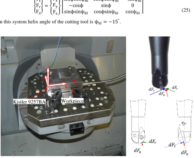
For approval of the proposed iterative method and analysis of non-linear effects, a series of tests were carried out. Milling pre-tests of workpiece (steel C35) with different lead angles (from 0° up to 60°) were carried out on a 5-axis milling machine Deckel Maho DMU 50 eVolution. During these pre-tests spindle speed was 3900 rpm and 4485 rpm; radial depth of cut was 0.5 mm and 1.0 mm. Pre-tests were carried out with Sandvik Coromant 2-flute ball end mill CoroMill 216 R216-10A16-050 with inserts R216-10 02 E-M 1010; mill diameter is Ø10 mm and free length is 49 mm (modal stiffness k = 7519 N/mm). Cutting scheme was slotting, climb and conventional milling. In the process of cutting, force components Fx, Fy and Fz were measured with Kistler 9257BA dynamometer as shown in a Fig. 7. Feeding was
{ Ft Fr Fa} = { Fx Fy Fz } [
sinϕcosψhl cosϕcosψhl −sinψhl
−cosϕ sinϕ 0
sinϕsinψhl cosϕsinψhl cosψhl
] (
(25) In this system helix angle of the cutting tool is ψhl = −15°.
Fig. 7 Cutting force experimental setup
These pre-tests gave an information about effective cutting force influence on tangential cutting force coefficient Kt [N/mm2] and lead angle influence on dimensionless radial cutting force coefficient Kr.
It had been determined that tangential cutting force coefficient decreases as cutting force increases. It corresponds with classical representation of high-speed machining. Thus, Kt decreases linearly from 5470 N/mm² to 3364 N/mm² as effective cutting velocity increases linearly from 53 m/min to 139 m/min. Experimental data are relevant to predicted Kt with an accuracy of ±5%. Radial cutting force coefficient increases as lead angle increases. For 30° Kr(30∘) = 0.16 and for 45° K
r(45∘) = 0.25.
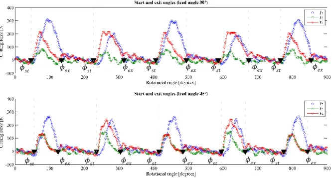
For instance, cutting force components are shown in Fig. 8. The initial conditions of this pretest are the next: lead angles equal 30° and 45° respectively; radial allowance ap,r equals
0.5 mm; radial depth of cut ae equals 4.36 mm (slot-milling condition); spindle speed equals
3900 rpm; feed-per-tooth equals 0.14 mm. Thus, calculated effective cutting velocity equals 100 m/min (lead angle is 30°) and 116 m/min (lead angle is 45°); start and exit angles equal
x
y
z
Kistler 9257BA Workpiece
𝑑𝐹𝑎 𝑑𝐹𝑟 𝑑𝐹 𝑡 𝑑𝐹𝑎 𝑑𝐹𝑎 𝑑𝐹𝑟 𝑑𝐹𝑡 𝜓ℎ𝑙
46° and 134° (lead angle is 30°), and 55° and 125° (lead angle is 45°), respectively. Time of cut equals 0.004 s (lead angle is 30°) and 0.003 s (lead angle is 45°).
Fig. 8 Tangential (blue line), radial (green line) and axial (red line) cutting force components
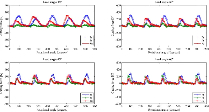
Tangential Ft, radial Fr and axial Fa cutting force components for different lead angles are shown in a Fig. 9. They are represented with blue, green and red lines, respectively. Radial components increase as lead angle increases. For instance, when lead angle equals 15°, radial
component is about 0. At the same time, axial components decrease. For instance, when lead angle is 15°, axial component almost equals tangential component. When lead angle is 60°,
axial component is less than radial component. Hence, it can be expected that cutting stability will go down if lead angle is increased.
𝜙𝑠𝑡 𝜙𝑒𝑥 𝜙𝑠𝑡 𝜙𝑒𝑥 𝜙𝑠𝑡 𝜙𝑒𝑥 𝜙𝑠𝑡 𝜙𝑒𝑥 𝜙𝑠𝑡 𝜙𝑒𝑥
Fig. 9 Cutting force components for various lead angles (15° 30° 45° 60°) in slot-milling
3.2 Cutting tool oscillations
Before machining, hammer impact tests were made. The corresponding frequency response functions (FRF) of the tool was obtained by a hammer impact tests using an instrumented hammer (2302-10, Endevco), a velocimeter laser (VH300+, Ometron) and a data acquisition system (Pulse, Brüel & Kjær). Measured modal stiffness 𝑘 = 2815 𝑁/𝑚𝑚; modal natural frequency of the system 𝑓𝑛 = 864 𝐻𝑧 and modal damping 𝜁 = 0.012 are collected in Table 1.
k fn
1.2 % 2815 N/mm 864 Hz
Table 1 Modal parameters identified
Fig. 10 shows the experimental setup. During machining, the vibration of the main system (1), which includes ball end mill (2) and workpiece (3) was measured by the velocimeter laser (4), the signal was collected by a conditioner (5) and stored in a personal computer (6).
a) b)
Fig. 10 Experimental setup: a) photo of setup; b) principal scheme of setup
4. Analysis of results
4.1 Stability lobes
Plotted stability lobes diagrams (Fig. 11-14) have been verified in a range of effective cutting velocity from 80 m/min to 150 m/min. Tests were carried out for slot-milling and up-milling on two workpieces with lead angles of 30○ and 45○, respectively. Radial depth of cut for slot-milling and up-slot-milling was obtained, respectively, as:
𝑎𝑒 = 2√𝑟2− (𝑟 − 𝑎 𝑝,𝑟) 2 (26) 𝑎𝑒 = √𝑟2− (𝑟 − 𝑎𝑝,𝑟) 2 (27)
1) 0.15 mm; 4800 rpm 2) 0.20 mm; 5200 rpm 3) 0.20 mm; 5400 rpm
Fig. 11 Experimental stability for slot-milling (lead angle 30°), stable tests results are marked with green ○,
limited stable tests results are marked with blue ▽, unstable tests results are marked with red ✕
In a Fig. 11 test results for slot-milling with lead angle of 30° are shown. In the tests №1 (0.15 mm; 4800 rpm) and №2 (0.20 mm; 5200 rpm) tooth pass excitation frequencies are dominated. These are limited stable and stable, respectively. In the test №3 natural frequency has much higher magnitude. This is unstable self-oscillation (chatter). Wavelike tool mark and time–frequency representation indicates the same.
1
1) 0.20 mm; 5200 rpm 2) 0.25 mm; 5200 rpm 3) 0.20 mm; 5400 rpm
Fig. 12 Experimental stability for slot-milling (lead angle 45°), stable tests results are marked with green ○,
limited stable tests results are marked with blue ▽, unstable tests results are marked with red ✕
In a Fig. 12 test results for slot-milling with lead angle 45° are shown. Test №1 (0.20 mm; 5200 rpm) demonstrates stable oscillation with tooth pass frequencies. High magnitude of the natural frequency oscillation, TFR-analysis and wavelike tool mark indicate chatter in the tests №2 (0.25 mm; 5200 rpm) and №3 (0.20 mm; 5400 rpm). In the test №2 higher harmonics also has place.
Test results for up-milling with lead angles 30° and 45° are presented in Fig. 13 and Fig. 14. Quasi-periodic stable oscillations are typical for up-milling. This can be explained by additional impact load, which is inherent in conventional milling, when tooth of the cutting tool leaves workpiece. Thus, magnitude of free flight oscillation grows up instantaneous after impact excitation (tooth leaving of workpiece). As previously noted, during ball-end milling
1 2
there is time stretched impact excitation. This kind of stability is according to supercritical Hopf bifurcation.
Fig. 13 Experimental stability for up-milling (lead angle 30°), stable tests results are marked with green ○; limited
stable tests results are marked with blue ▽; unstable tests results are marked with red ✕
Fig. 14 Experimental stability for up-milling (lead angle 45°), stable tests results are marked with green ○; limited
4.2 Discussion
More than 80 cutting tests have been conducted to emphasize the behaviour of inclined surface. A quite good agreement is observed between simulations and machining tests. The discrepancies between the experiment and the modelling are observed for some spindle speed, in particular for up-milling (lead angle 30°) at 4600 rpm, see Fig. 13. It is presently not clear what causes these discrepancies. A possible cause could be due to the non-linear variation of damping of the system. Its variation in turn may be based on a host of factors: variations of friction force, elastic properties, flank wear growth, temperature increase in cutting zone, and so on and so forth.
5. Conclusions
This paper presents a study of warped surfaces machining on milling machines with ball end mills. A specific model based on the classical stability lobe theory was use and improved with more important aspects. The non-linear effect of radial allowance on the contact angle was integrated by an original averaging method. The cutting coefficients are updated during changing of effective radius and cutting velocity. This modelling allows predicting the stability lobe on inclined surface more accurately but easy to adjust in a real industrial process.
An original experimental procedure was developed in order to compute the cutting coefficient for various inclined surfaces. In real context, the cutting forces are measured by a standard dynamometer with various inclinations. The cutting coefficients are non-constant, and large amplitude of variation is observed as function of the tilt surface.
More complete experimental analysis was conducted in order to study the effect of machining parameters on the stability of climb milling. The lead angle has a direct impact on cutting stability, the greater the angle decreases more the stability increases.
The comparison between experiment and simulation show good correlation for the prediction of the depth of cut without chatter. Therefore, the improvement in the simulation of inclined surface inclined surfaces machining on milling machines with ball end mills needs the development non-linear damping models.
References
[1] Tobias SA, Fishwick W (1958) Theory of regenerative machine tool chatter. Engineer-London 205:199–203;238–239
[2] Altintas Y, Budak E (1995) Analytical prediction of stability lobes in milling. CIRP Ann-Manuf Techn 44:357–362
[3] Budak E (2006) Analytical models for high performance milling – Part I: cutting forces, structural deformations and tolerance integrity. Int J Mach Tool Manu 46:1478–1488
[4] Budak E (2006) Analytical models for high performance milling – Part II: process dynamics and stability. Int J Mach Tool Manu 46:1489–1499
[5] Altintas Y, Shamoto E, Lee P, Budak E (1999) Analytical prediction of stability lobes in ball end milling. J Manuf Sci E-T ASME 121:586–592
[6] Altintas Y (2001) Analytical prediction of three dimensional chatter stability in milling. JSME Int J C-Mech SY 44:717–723
[7] Ozturk E, Tunc LT, Budak E (2009) Investigation of lead and tilt angle effects in 5-axis ball-end milling processes. Int J Mach Tool Manu 49:1053–1062
[8] Mousseigne M, Landon Y, Seguy S, Dessein G, Redonnet JM (2013) Predicting the dynamic behaviour of torus milling tools when climb milling using the stability lobes theory. Int J Mach Tool Manu 65:47–57
[9] Chao S, Altintas Y (2016) Chatter free tool orientations in 5-axis ball-end milling. Int J Mach Tool Manu 106:89–97
[10] Davies MA, Pratt JR, Dutterer B, Burns TJ (2002) Stability prediction for low radial immersion milling. J Manuf Sci E-T ASME 124:217–225
[11] Bayly PV, Halley JE, Mann BP, Davies MA (2003) Stability of interrupted cutting by temporal finite element analysis. J Manuf Sci E-T ASME 125:220–225
[12] Insperger T, Mann BP, Stépán G, Bayly P V (2003) Stability of up-milling and down-milling, part 1: alternative analytical methods. Int J Mach Tool Manu 43:25–34
[13] Insperger T, Stépán G (2004) Updated semi-discretization method for periodic delay-differential equations with discrete delay. Int J Numer Meth Eng 61:117–141
[14] Merdol SD, Altintas Y (2004) Multi frequency solution of chatter stability for low immersion milling. J Manuf Sci E-T ASME 126:459–466
[15] Mann BP, Insperger T, Bayly PV, Stépán G (2003) Stability of up-milling and down-milling, part 2: experimental verification. Int J Mach Tool Manu 43:35–40
[16] Insperger T, Mann BP, Surmann T, Stépán G (2008) On the chatter frequencies of milling processes with runout. Int J Mach Tool Manu 48:1081–1089
[17] Zhang X, ·Zhang J, Pang B, Wu DD, Zheng XW, Zhao WH (2016) An efficient approach for milling dynamics modeling and analysis with varying time delay and cutter runout effect. Int J Adv Manuf Tech doi:10.1007/s00170-016-8671-8
[18] Zatarain M, Muñoa J, Peigné G, Insperger T (2006) Analysis of the influence of mill helix angle on chatter stability. CIRP Ann-Manuf Techn 55:365–368
[19] Seguy S, Arnaud S, Insperger T (2014) Chatter in interrupted turning with geometrical defects: An industial case study. Int J Adv Manuf Tech 75:45–56
[20] Insperger T, Stépán G, Bayly PV, Mann BP (2003) Multiple chatter frequencies in milling processes. J Sound Vib 262:333–345
[21] Stépán G, Szalai R, Insperger T (2005) Nonlinear dynamics of high-speed milling subjected to regenerative effect. In: Radons G and Neugebauer R (eds) Nonlinear Dynamics of Production Systems. Wiley-VCH Verlag, Weinheim doi: 10.1002/3527602585.ch7
[22] Stépán G, Insperger T, Szalai R (2005) Delay, parametric excitation, and the nonlinear dynamics of cutting processes. Int J Bifurcat Chaos 15:2783–2798
[23] Seguy S, Insperger T, Arnaud L, Dessein G, Peigné G (2011) Suppression of period doubling chatter in high-speed milling by spindle speed variation. Mach Sci Technol 15:153–171
[24] Insperger T (2010) Full-discretization and semi-discretization for milling stability prediction: Some comments. Int J Mach Tool Manu 50:658–662
[25] Ozoegwu CG, Omenyi SN, Ofochebe SM (2015) Hyper-third order full-discretization methods in milling stability prediction. Int J Mach Tool Manu 92:1–9
[26] Tang X, Peng F, Yan R, Gong Y, Li Y, Jiang L (2016) Accurate and efficient prediction of milling stability with updated full-discretization method. Int J Adv Manuf Tech doi: 10.1007/s00170-016-8923-7
[27] Wang S, Geng L, Zhang Y, Liu K, Ng T (2015) Chatter-free cutter postures in five-axis machining. P I Mech Eng B-J Eng doi: 10.1177/0954405415615761
[28] Campomanes ML, Altintas Y (2003) An improved time domain simulation for dynamic milling at small radial immersions. J Manuf Sci E-T ASME 125:416–422
[29] Liu X, Cheng K (2005) Modelling the machining of peripheral milling. Int J Mach Tool Manu 45:1301–1320
[30] Surmann T, Enk D (2007) Simulation of milling tool vibration trajectories along changing engagement conditions. Int J Mach Tool Manu 47:1442–1448
[31] Arnaud L, Gonzalo O, Seguy S, Jauregi H, Peigné G (2011) Simulation of low rigidity part machining applied to thin walled structures. Int J Adv Manuf Tech 54:479–488
[32] Ahmadi K, Ismail F (2011) Analytical stability lobes including nonlinear process damping effect on machining chatter. Int J Mach Tool Manu 51:296–308
[34] Shtehin OO (2014) Vyznachennya kutiv vrizannya ta vykhodu pry obrobtsi pokhylykh poverkhon sferychnymy kintsevimi frezamy [Definition of start and exit angles in ball end milling of inclined surfaces]. Visnyk ZHDTU – Reporter of ZSTU 3(70) 62–67 [in Ukrainian]
[35] Cosma M (2007) Horizontal path strategy for 3D-CAD analysis of chip area in 3-axes ball nose end milling. 7th International Multidisciplinary Conference, Baia Mare, Romania
List of Figures Captions
Fig. 1 Start and exit angles in end mill machining, a) down-milling with flat end mill, b) down-milling with ball end mill (lead angle 30°), c) down-milling with ball end mill (lead angle 45°), d) up-milling with flat end mill, e) up-milling with ball end mill (lead angle 30°), f) up-milling with ball end mill (lead angle 45°)
Fig. 2 Single Degree Of Freedom model of cutting with ball end mill, a) static representation, b) dynamic representation
Fig. 3 Difference between radial allowance and axial depth of cut in a case of inclined surface ball end milling Fig. 4 Non-linear effect of radial allowance on the contact angle
Fig. 5 Iterative plotting of stability lobes diagrams for ball end milling
Fig. 6 Comparison of classical approach and proposed method for stability lobes in slot-milling with 30° and 45° Fig. 7 Cutting force experimental setup
Fig. 8 Tangential (blue line), radial (green line) and axial (red line) cutting force components Fig. 9 Cutting force components for various lead angles (15° 30° 45° 60°) in slot-milling Fig. 10 Experimental setup: a) photo of setup; b) principal scheme of setup
Fig. 11 Experimental stability for slot-milling (lead angle 30°), stable tests results are marked with green ○; limited stable tests results are marked with blue ▽; unstable tests results are marked with red ✕
Fig. 12 Experimental stability for slot-milling (lead angle 45°), stable tests results are marked with green ○; limited stable tests results are marked with blue ▽; unstable tests results are marked with red
Fig. 13 Experimental stability for up-milling (lead angle 30°), stable tests results are marked with green ○; limited stable tests results are marked with blue ▽; unstable tests results are marked with red ✕
Fig. 14 Experimental stability for up-milling (lead angle 45°), stable tests results are marked with green ○; limited stable tests results are marked with blue ▽; unstable tests results are marked with red ✕
List of Tables
Table 1 Modal parameters identified
k fn