HAL Id: halshs-01184598
https://halshs.archives-ouvertes.fr/halshs-01184598
Submitted on 18 Oct 2019
HAL is a multi-disciplinary open access archive for the deposit and dissemination of sci-entific research documents, whether they are pub-lished or not. The documents may come from teaching and research institutions in France or abroad, or from public or private research centers.
L’archive ouverte pluridisciplinaire HAL, est destinée au dépôt et à la diffusion de documents scientifiques de niveau recherche, publiés ou non, émanant des établissements d’enseignement et de recherche français ou étrangers, des laboratoires publics ou privés.
The European Climate Policy is Ambitious: Myth or
Reality?
Catherine Benjamin, Isabelle Cadoret David, Marie-Hélène Hubert
To cite this version:
Catherine Benjamin, Isabelle Cadoret David, Marie-Hélène Hubert. The European Climate Policy is Ambitious: Myth or Reality?. Revue d’Economie Politique, Dalloz, 2015, 125 (5), pp.731-753. �10.3917/redp.255.0731�. �halshs-01184598�
The European Climate Policy is Ambitious: Myth or
Reality?
Catherine Benjamin, Isabelle Cadoret and Marie-H´
el`
ene Hubert
∗November 14, 2018
∗Benjamin: CREM UMR CNRS 6211, Universit´e de Rennes 1, 7 Place Hoche, 35065 Rennes, FRANCE
email: [email protected]; Cadoret: CREM UMR CNRS 6211, Universit´e de Rennes 1, 7 Place Hoche, 35065 Rennes, FRANCE email: [email protected]; Corresponding author: Hubert: CREM UMR CNRS 6211, Universit´e de Rennes 1, 7 Place Hoche, 35065 Rennes, FRANCE email: [email protected]. We are very grateful to the editors, Jean-Fran¸cois Bourguignon and Marie-Claire Villeval, together with two anonymous referees for their insightful comments and suggestions that led to a substantial improvement of the paper. We would like also to thank the participants at the 63rd Annual Congress of AFSE and at the 5th World Congress of Environmental and Resource Economists for their useful comments.
Abstract
We investigate carbon emission trends among EU Member States by testing the assump-tion of β-type convergence in per capita CO2 emissions, conditional upon per capita
output, world oil price, energy use per capita and investment in renewable energy. Our study supports the assumption of conditional convergence among all EU Member States. It should take around 10 years for the EU-15 countries to stabilize their per capita emis-sions. This result does not change if we include the new Member States in the sample. We also find that the emission growth/income relation is strictly negative, indicating that EU-15 countries switched to a less carbon intensive economy starting from the early 1990s. This result remains robust when the new Member States are included. We there-fore argue that the decline in EU carbon emissions is a long-term trend and not a result of the economic crisis. We then discuss the effectiveness of climate and energy policies and the EU burden-sharing agreement. Some countries like Germany, Great Britain and France can meet their carbon targets without adopting more aggressive climate and en-ergy policies by 2020. Other EU-15 Member States can reduce their domestic emissions beyond their targets if they adopt energy-efficient technologies. Most of the new Member States emit much less than their domestic targets even when per capita income and oil price increase.
Keywords: Convergence, Dynamic Panel Data Models, Carbon Dioxide, European Union Cli-mate Policy.
JEL Codes: Q42, Q48
Abstract
Nous analysons les ´evolutions dans le long terme des ´emissions de carbone en Europe en s’appuyant sur le concept de convergence des ´emissions de CO2 par tˆete conditionnelle
au revenu par tˆete, au prix mondial du p´etrole, `a la consommation ´energ´etique par tˆete et `a l’investissement en ´energie renouvelable. L’hypth`ese de convergence conditionnelle entre les pays de l’Union Europ`eenne est v´erifi´ee. Les pays de l’UE-15 devraient stabiliser leurs ´emissions d’ici 10 ans. Ce r´esultat est inchang´e si nous incluons les nouveaux pays Membres dans l’´echantilllon. Les ´economies de l’Union Europ´eenne sont peu intensives en carbone, i.e., la relation croissance des ´emissions/revenu est strictement n´egative. Ce r´esultat est robuste si nous incluons les nouveaux Etats membres. Puis, nous discutons de l’efficacit´e des politiques ´energ´etiques et climatiques et de la r´epartition de l’effort d’abattement entre les diff´erents pays Membres. L’Allemagne, la Grande-Bretagne et la France peuvent atteindre leur cible de carbone sans r´ealiser d’efforts suppl´ementaires. Les autres Etats membres de l’UE-15 peuvent atteindre la cible en r´ealisant des investisse-ments dans les ´energies renouvelables et en am´eliorant leur efficacit´e ´energ´etique. Les ´
emissions des nouveaux Etats membres devraient ˆetre inf´erieures `a leur valeur cible malgr´e l’augmentation du revenu par tˆete et du prix de p´etrole.
Mots-cl´es : Convergence, Mod`ele de Panel Dynamique, Dioxyde de Carbone, Politique Clima-tique Europ´eenne.
1
Introduction
The former European Commission president, Jose Manuel Barroso, recently declared that
“No player in the world is as ambitious as the EU when it comes to cutting greenhouse gas
emissions”. The European Union (EU) was the only region of the Annex I countries to achieve
its Kyoto target. In 2008-2012, total greenhouse gas (GHG) emissions were 10.6% below their
1990 levels while the Kyoto Protocol had imposed a reduction of only 8%.1 Some argue that this good performance is the result of the financial and economic crisis. However, it is worth noting
that most of the EU countries were in track to meet their Kyoto targets in 2004-2008 (Eboli
and Davide, 2012). In 2009, despite a slow down in international negotiations, the European
Commission decided to embark in new commitments by defining three objectives for 2020: a
20% GHG emissions reduction below their 1990 levels, an increase in the share of renewable
energy source over total energy production to at least 20%, and a 20% increase in energy
efficiency.2 On 24 October 2014, the Commission sought to reinforce its drive for a low carbon economy by setting new targets for 2030, including a reduction in domestic GHG emissions by
40% below the 1990 levels, an increase in the share of renewable sources in the production of
energy to 27% and a rise in energy efficiency by 27%. In this context, the role being played
by the EU is quite unique and raises some questions: i) is this carbon emission reduction a
long-term trend, i.e., has the EU economy already switched to a low carbon economy? ii) if so,
are the carbon emission targets set by the EU ambitious enough, or possibly too ambitious?
A detailed examination of the long-term carbon emission trends across the EU Member States
is required to address these issues.
To investigate long-term carbon emission trends, we apply the econometric framework
based on the Solow’s model, which is used in the macroeconomic literature on income
conver-1This good result hides substantial differences between Member States. Sweden, Germany, and France
succeeded in meeting their emissions reduction target while Luxembourg and Austria failed to do so. However, the largest decrease in carbon emissions occurred in the new Member States although they only signed a voluntary agreement in 2004 when they joined the EU (except Cyprus and Malta). EU carbon emissions decreased by around 15% below their 1990 levels.
2The generic definition of energy efficiency is “a way of managing and restraining the growth in energy
consumption. Something is more energy efficient if it delivers more services for the same energy input, or the same services for less energy input” (IEA, 2013). According to the Energy Efficiency Directive, EU Member States are supposed to increase their energy efficiency by 20%, e.g., to reduce their primary energy consumption by 20% (page 2, Directive 2012(2012)). In the rest of the paper, we refer to energy efficiency as the decrease in primary energy consumption.
gence (Baumol (1986), Barro and Sala-i Martin (1992) and Quah (1996)).3 Its key prediction is that per capita income among economies should converge if economic characteristics such as
savings rate or technological progress rate are controlled. This framework has been extended
to explain pollution emissions across different countries (Brock and Taylor, 2010). Numerous
studies have tested the hypothesis of convergence in pollution among different regions or
coun-tries. In a seminal paper, Strazicich and List (2003) test the convergence of per capita CO2
emissions among 21 industrialized countries between 1960 and 1997. Using annual data and
employing two econometric methodologies (cross-sectional approach and unit root test), they
show that per capita CO2 emissions have converged. Ord´as Criado et al. (2011) extend the
Ramsey Model to endogenous carbon emission reduction. Their empirical results confirm the
existence of a defensive effect (growth rate of per capita emissions is negatively related to the
initial level of per capita emissions) and a scale effect (growth rate of per capita emissions is
positively related to the growth rate of per capita output) for two pollutants (sulfur oxides
and nitrogen oxides) in 25 European countries over the period 1980-2005. Ord´as Criado and
Grether (2011) examine cross-country convergence process for per capita CO2 emissions with
a panel of 166 world areas spanning the years 1980-2005. Based on non-parametric
methodolo-gies, they identify clusters of converging economies. Europe, Central Asia, Sub-Saharan Africa
and the low-income countries converge toward lower per capita emissions in the long run, while
those for OECD, EU-15 and the G20 are close to their current distribution. Jobert et al.(2010)
investigate the convergence hypothesis in 22 European countries over the 1971-2006 period. By
using Bayesian shrinkage method, their results support the assumption of absolute convergence
in per capita CO2 emissions. Since countries differ in both their speed and volatility of
conver-gence in emissions, different groups of countries having different emissions characteristics can
be identified.4
3SeeDurlauf et al.(2005) for a review of the literature.
4The first group, called “volatile polluters”, is characterized by a high speed of convergence and their emission
levels show a high variation in time. This group is mainly composed of Northern European countries. The second group, qualified as “ecologists”, is composed of Eastern countries and three EU-15 countries (France, Germany, Ireland). Their initial level of per capita emissions is high, but, they show a decreasing trend in per capita CO2 emissions especially after 1990. South European countries (except Portugal) belongs to the third
group named “Club Med Polluters”. They show a low initial emissions level, but an increasing trend for this variable. Finally, Portugal and Turkey form the fourth group. They are characterized by a low convergence process and their carbon emissions increase sharply.
In the first step of our analysis, we test the assumption of convergence in per capita
emissions among the 15 Member Sates of the European Union (i.e., the histprcal Member
States) conditional on their level of per capita income, world oil price and energy use per
capita using a dynamic panel data set over the period 1960-2009. Our results confirm that the
per capita emissions have conditionally converged and that the EU-15 countries should stabilize
their per capita emissions in roughly 10 years, i.e., around 2020/2024. This framework also
allows us to examine whether the historical Member States have switched to a low carbon
economy by testing the existence of a structural break in the relation between emission growth
and per capita income. Before the 1990s, an inverted U-shaped exists. After the 1990s, the
emission growth/GDP per capita relationship is strictly negative. In a second step, we explore
the process of convergence in per capita emissions conditional on their level of per capita
income, world oil price, energy use per capita and investment in renewable sources among all
EU members (EU-15 countries and new Member States) over the period 1990-2009.5 The speed of convergence is robust to the inclusion of the new Member States, i.e., all EU Member States
should stabilize their per capita emissions in about 10 years. In addition, for all Member States
a higher level of GDP per capita leads to a decrease in emission growth although this effect
is limited. The main contribution of this paper is to use our regression results to investigate
the effectiveness of the EU energy and climate policies by employing bootstrap method. This
allows us to identify: i)the extent to which the EU members may achieve their domestic
carbon emission reduction target by 2020 and ii)the main drivers (macroeconomic variables or
climate and energy policies) that could affect the efforts EU members must make to achieve
their 2020-targets. Our results show that Great-Britain, Germany and France will reach their
carbon target without additional investment in renewable energy or improvements in energy
efficiency in around 2020. Other member States should invest more in renewable energy or in
energy efficiency to reach their 2020-commitment. For instance, Luxemburg and Sweden should
increase their production of renewable energy by 20%. However, improved energy efficiency
appears to be a better climate policy lever. With the exception of Ireland and Finland, all of
the EU-15 Member States can hit their domestic targets by investing in more energy efficient
5In the rest of the paper, we name indifferently the EU-15 countries as the historical Member States or
technologies. However, most of the Eastern European countries are already emitting less than
their targets level, and will honor their 2020-commitments even if per capita income or oil price
increase.
The rest of the paper proceeds as follows. Section 2 presents the European energy and
climate policies. Section 3 describes our econometric methodology and data. Results are
discussed in section 4. Finally, section 5 concludes.
2
Policy background
In this section, we discuss the European Union energy and climate policies since the end
of the Second World War.
The achievements of the EU energy and climate policies
The history of the European Union is rooted in energy issues (Keppler, 2007). The
Treaty establishing the European Coal and Steel Community (ECSC) was signed in 1951. It
set up a common customs union for two commodities (coal and steel) which were essential for
warfare and reconstruction alike. Six years later, the European Atomic Energy Community
(EURATOM) was established to extend the power of the ECSC to other sources of energy and
in particular nuclear power. The first oil crisis highlighted the need to ensure energy security.
In 1974, the European Council adopted a program to diversify energy sources. Later, in 1995,
the EU attempted to liberalize the energy market to promote competition and the security of
supply. In the late 1990s, EU energy policy began to focus on climate change in addition to
improving energy security. In 1997, under the Kyoto Protocol, the EU-15 agreed to reduce
its GHG emissions by 8% below their 1990 levels over the period 2008-2012. Specific targets
were defined for each Member States based on their energy mix and economic performance.
Countries where the share of fossil fuel in the energy was high such as Luxembourg, Germany
and Austria had to substantially reduce their carbon emissions. Countries like Finland and
France where the share of nuclear power in the production of electricity already was high, had
and Portugal could increase their carbon emissions. To meet the overall 8% reduction target,
two key Directives on Renewable Energy were established. The 2001 Directive quantified an
overall target for electricity produced from renewable energy.6 The 2003 Directive reinforced these objectives in many ways. A mandate on biofuel use, minimum taxation rates for energy
products, electricity and heating fuels were established. The most important policy tool was
the creation of the carbon exchange trading market in 2005 which is often considered as the
centerpiece of the EU’s climate policy.
The challenges of the EU energy and climate policies
To prepare an EU climate policy after the end of the Kyoto Protocol, the European
Commission defined new and ambitious commitments for carbon emissions reductions in 2007.
Quantifiable targets, the so-called 20/20/20, were set up: a reduction in EU GHG emissions of
at least 20% below 1990 levels; 20% of EU energy production to come from renewable resources
and a 20% reduction in primary energy use, to be achieved by improving energy efficiency. The
overall target on carbon emissions was translated into national targets which took into account
the per capita income and energy mix of each Member State (see figure1). Historical Member
States must make greater efforts to reduce their carbon emissions while the emissions of Eastern
European Member States can increase. The EU is on track to meet its overall renewable energy
target since the share of renewable energy in gross final energy production rises from around
8% in 2004 to 12% in 2010 and to over 14% in 2014 (EUROSTAT, 2013). In contrast, much
work remains to be done in terms of energy efficiency. Primary energy use increased by around
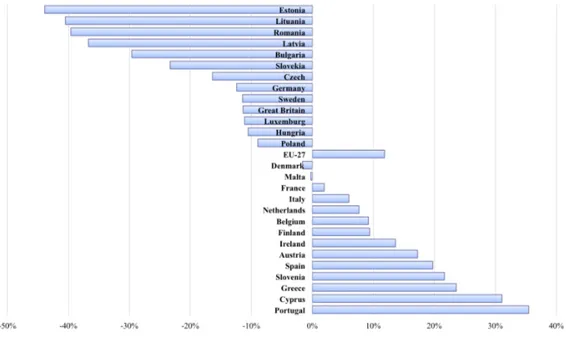
12% from 1990 to 2009 in the EU. This number hides significant disparities. Figure 2 shows
the growth rates of primary energy use from 1990 to 2009 for each EU Member State. The
largest declines in the primary energy use occurred in Eastern European countries while the
largest increases occurred in the historical Member States. After 1990, drastic reductions in
carbon emissions have been observed. Zugravu et al. (2010) identify several factors to explain
this tremendous drop, including a decrease in industry’s share of GDP, investments in clean
6The Directive set an overall target of 22% of electricity produced from renewable by 2010. Specific national
technologies and the political institutions. In October 2014, the European Commission defined
ambitious targets for 2030 like the reduction of domestic carbon emissions, the increase in the
share of renewable sources in the total production of energy and the improvement in energy
efficiency (European Council, 2014).
Figure 1: CO2 emission reduction targets for EU Member States by 2020 (expressed in
percentage change in 2020 compared to 1990 levels)
Source: EEA(2013b), page 102; Notes: The emission reduction targets compared to their emission in 1990 are established by the European Commission based on the economic development and energy mix of each EU Member States.
3
Econometric strategy and data
Before defining our econometric strategy and the data we use, we analyze graphically
the process of absolute convergence in per capita emissions among the EU Member States.
According to this concept, the countries with lower per capita emissions levels are expected to
experience higher growth rates of pollution. Hence, they may catch-up with the most polluting
Figure 2: Percentage change in energy use per capita for EU Member States from 1990 to 2009
Source: EUROSTAT(2013), Notes: According toEUROSTAT(2013), by primary energy consumption is meant the Gross Inland Consumption excluding all non-energy use of energy carriers (e.g. natural gas used not for combustion but for producing chemicals). This quantity is relevant for measuring the true energy consumption and for comparing it to the Europe 2020 targets.
Preliminary data analysis
To examine the potential impact of EU energy and climate policies on the carbon emission
trends from the early 1960s, we analyze the convergence of per capita CO2 emissions among
the EU-15 countries. Figure 3shows the absolute convergence in per capita emissions for each
EU-15 country over three periods: 1960-2009 (figure on the top left), 1960-1989 (figure on
the top right) and the 1990-2009 (figure on the bottom left). We split the sample into two
sub-periods: 1960-1989 and 1990-2009 because many countries adopted environmental policies
in the early 1990s. We can clearly see that from 1960 to 2009, the less polluting countries
in 1960 (Greece and Portugal) experienced the highest growth rates of per capita emissions.
A group of countries located in the bottom-right below the horizontal black line is formed
by Luxembourg, Germany, Sweden and France. They exhibited a negative emission growth.
Before the 1990s, only Sweden and Great-Britain had a negative per capita emission growth
rate. After the 1990s, the growth rates of per capita emissions are negative for most of the
EU-15 countries. Only Portugal, Greece, Ireland and Finland showed an increasing trend.
second period than over the first period. The data analysis over the whole period seems to
reveal that the EU economy switched to a low carbon economy before the implementation of
the EU climate policies in 2001.
Figure 3: CO2 emission growth (1960-2009) versus initial per capita CO2 emissions (EU-15
countries)
Source: Per capita carbon emissions are from World Bank (World Bank,2013). Notes: Growth of CO2emissions per capita is the
average annual growth rate of CO2 emissions per capita over the period. We use the following abbreviations: Aus: Austria; Bel:
Belgium; Den: Denmark; Fin: Finland; Fra: France; Ger: Germany; G-Br: Great-Britain; Gre: Greece; Ire: Ireland; Ita: Italy; Lux: Luxemburg; Net: The Netherlands; Por: Portugal; Spa: Spain; Swe: Sweden.
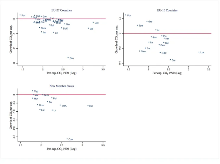
Then, we include the New Member States to our sample since they are committed to
reduce their emissions by 2020. Figure4shows the absolute convergence in per capita emissions
for all Member States (figure on the top left), EU-15 countries (figure on the top right) and new
Member States (figure on the bottom left). Although the new Member States are less wealthy
than the historical Member States, their per capita emissions in 1990 do not differ substantially
exhibit the highest decrease in carbon emissions. The average rate of decrease in per capita
emissions among the historical Members does not exceed 0.5% while it reaches 1.5% among
the new Member States.
Figure 4: CO2 emission growth (1990-2009) versus initial per capita CO2 emissions (EU
countries)
Source: Per capita carbon emissions are from World Bank (World Bank,2013). Notes: Growth of CO2 emissions per capita is
the average annual growth rate of CO2 emissions per capita over the period. We use the following abbreviations: Aus: Austria;
Bel: Belgium; Den: Denmark; Fin: Finland; Fra: France; Ger: Germany; G-Br: Great-Britain; Gre: Greece; Ire: Ireland; Ita: Italy; Lux: Luxemburg; Net: The Netherlands; Por: Portugal; Spa: Spain; Swe: Sweden; Bul: Bulgaria; Cyp: Cyprus; Cze: Czech Republic; Est: Estonia; Hun: Hungary; Lat: Latvia; Lit: Lithuania; Mal: Malta; Pol: Poland; Rom: Romania; SloK: Slovakia; SloN: Slovenia.
Preliminary data analysis suggests that two trends may exist. The first is that the
decrease in carbon emissions observed in the EU may be a long term process. The second is
that the economic growth among the new Member States emissions has not generated high
emission growth. To test the existence of these trends, we borrow our econometric strategy
analyze the process of β-convergence in per capita emissions conditional on country specific
characteristics. As we can see on figure5, the emission growth (gCO2) is a declining function of
the initial level of carbon emissions (logCO02). It should converge to 0, we call the asymptotic value. However, this value can shift with country-specific characteristics and climate and energy
policies. For instance, we can except that climate and energy policies can cause a decrease in
the asymptotic value of per capita emissions and a shift to the new asymptotic value of carbon
emissions logCO2N.
Figure 5: β-convergence in per capita CO2 emissions conditional on country-specific
charac-teristics
Econometric strategy
As inOrd´as Criado et al.(2011), we construct a panel data based on five-year periods (T
= 5) to capture long-term adjustments. A critical step in the analysis of the β-convergence is
the choice of the vector of control variables since the latter are supposed to allow for country
differences in the time path of emissions (see figure 5). Many suggestions can be found in the
literature, for example, GDP per capita, energy prices, climate, industry’s share in GDP.7 In our study, we include four control variables to analyze the impact of macroeconomic shocks
and climate and energy policies on on the convergence process and on the asymptotic value of
7Strazicich and List (2003) chose four control variables (GDP per capita, price of gasoline, population
density and average temperature) to test the conditional convergence in 21 industrialized countries. To test the conditional convergence among 22 European States, Jobert et al.(2010) included three control variables: the GDP per capita, country population and industry’s share of GDP.
carbon emissions. First, the GDP per capita is employed as a measure of the wealth of the
country. As in Strazicich and List (2003), we assume that in the initial phase of the growth
process, i.e., for low levels of per capita GDP, emission growth tends to rise, and that once
the GDP per capita passes some threshold level, economic growth does not cause an increase
in carbon emissions. To capture this possible inverted U-shaped relation, we introduce a
quadratic term. We also introduce oil price which can be interpreted as a measure of fossil
fuel price. Higher energy prices make alternative and carbon free energy like wind, solar more
competitive. In the long run, they thus lead to lower rates of carbon emissions. The two
remaining control variables: energy use per capita and growth in the production of renewable
energy are introduced to capture the effects of the EU energy and climate policies. Growth
in the production of renewable sources is used as a proxy for investment in renewable sources.
The generic equation of conditional convergence is:
gCO2i,t = γi+ β log CO2i,t−T + α log GDPi,t+ δ log GDP
2 i,t
+ µlog(OilP rice)t+ θlogZi,t+ ξi,t (1)
where gCO2it is the annual average growth rate of carbon emissions, it is calculated as the
average log changes (1/T )log(CO2it/CO2i,t−T) over the period t-T to t; CO2i,t−T is the level
of CO2 per capita emissions at the beginning of the period t-T or the initial level of per
capita emissions,8 GDPi,t is the average GDP per capita in country i over the period t-T to
t, OilP ricet is the average world oil price over the period t-T to t, Zi,t is a vector of
time-varying country characteristics like energy use per capita and growth rate of the production of
renewable sources,9 ξi,t is the error term. We introduce country fixed-effects in order to take
into account heterogeneity across countries. The hypothesis of β-convergence is supported if
the coefficient β is significantly negative. The relation between per capita emission growth
and GDP per capita has inverted-U shape if α is significantly positive and δ is significantly
negative. The turning point is obtained by: − α 2δ.
8In the rest of the paper, we will use the term initial level of the variable to refer to the value of this variable
at the beginning of the period t-T.
9For each control variable, we calculate their average value over the period t-T to t. Data on the growth
In the first step of our analysis, we focus on the β-convergence among the EU-15 countries
with a panel set spanning 1960 to 2009.10 To test if a structural break exists in the relation between per capita emission growth and GDP per capita, we introduce a dummy variable PER1
which takes the value 1 over the period 1960-1989 and 0 otherwise. The following equation is
estimated:
gCO2i,t = γi+ β log CO2i,t−T + α1log GDPi,t+ α2log GDPi,t∗ P ER1
+ δ1log GDPi,t2 + δ2log GDPi,t2 ∗ P ER1 + µlog(OilP rice)t+ θ log Zi,t+ ξi,t (2)
If α2 and γ2 are significantly different from zero, a structural break exists. Otherwise, no
structural break exists.
In a second step, we extend our sample to all EU members by using a dynamic panel
set covering the period 1990-2009.11 The data set starts after 1990 since most of the new EU members emerged from the dissolution of the Union of Soviet Socialist Republics in 1991. Our
aim is to detect a structural difference between the historical EU members and the new EU
members. We introduce a dummy variable (NEU15) which takes the value 1 if the country i
is a new EU members and 0 otherwise. The following equation is estimated:
gCO2i,t = γ˜i+ ˜β log CO2i,t−T + ˜α1log GDPi,t+ ˜α2log GDPi,t∗ N EU 15
+ δ˜1log GDPi,t2 + ˜δ2log GDPi,t2 ∗ N EU 15 + ˜µlog(OilP rice)t+ ˜θ log Zi,t+ ˜ξi,t (3)
If ˜α2, and ˜δ2 are statistically different from zero, a structural difference exists between the two
groups of countries. Otherwise, no structural difference exists.
We first estimate the dynamic panel equations: equation (2) and equation (3) with the
Least Square Dummy Variable (LSDV); however, the estimator is biaised (Greene,2012). Two
estimation techniques exist to tackle with this problem. The first, GMM methods for dynamic
panels developed by Arellano and Bond(1991) andArellano and Bover(1995) has been widely
used in growth models. The second econometric method involves instrumental variable, and
10This data set includes 10 periods of five years: 1960-1964; 1965-1969; 1970-1974; 1975-1979; 1980-1984;
1985-1989; 1990-1994; 1995-1999; 2000-2004; 2005-2009.
11This data set includes 4 five-year periods: 1990-1994; 1995-1999; 2000-2004; 2005-2009. In July 2013,
Croatia joined the EU. However, we do not include this country in our data set since its carbon emissions represented less than 1% of EU emissions in 2010 (World Bank,2013).
is what we use in this paper in the form of IV-GMM estimators (Checherita-Westphal and
Rother, 2012). We prefer this second instrumental variable methodology since it allows us to
estimate a fixed effects model which controls for non-observable country characteristics. It is
crucial to estimate a fixed-effect model since our objective is to use the estimated coefficients
of this equation to i) the efforts each Member States should make to reach their targets and
ii) measure the potential role of climate and energy policies and macroeconomic shocks. We
instrument the initial level of per capita emissions for each EU Member State through the
initial energy use per capita.12
Data
To estimate equation (2) and equation (3), we build two data sets named respectively
Panel A and Panel B. The World Bank (World Bank, 2013) provides a full data set on per
capita carbon emissions measured in metric tons per capita from 1960 for each country of
the world. According to the definition given by the World Bank, “carbon emissions are those
stemming from the burning of fuels and the manufacture of cement. They include carbon
dioxide produced during consumption of solid, liquid, and gas fuels and gas flaring”.13 Per capita Gross Domestic Product (GDP) is from the Penn World Table (Heston et al., 2012). It
is deflated by country into 2005 US dollars and calculated in purchasing power parity. Oil price
is from the World Bank (2014). It is calculated as the average spot price of Brent, Dubai and
West Texas Intermediate and expressed in 2005 US dollars. According to EUROSTAT(2013),
primary energy consumption means the Gross Inland Consumption excluding all non-energy
use of energy carriers (e.g. natural gas used not for combustion but for producing chemicals).
It is expressed in tons oil equivalent (or, toe). The growth rate of the production of renewable
sources is calculated from EUROSTAT (2013), it is available only after 1990.
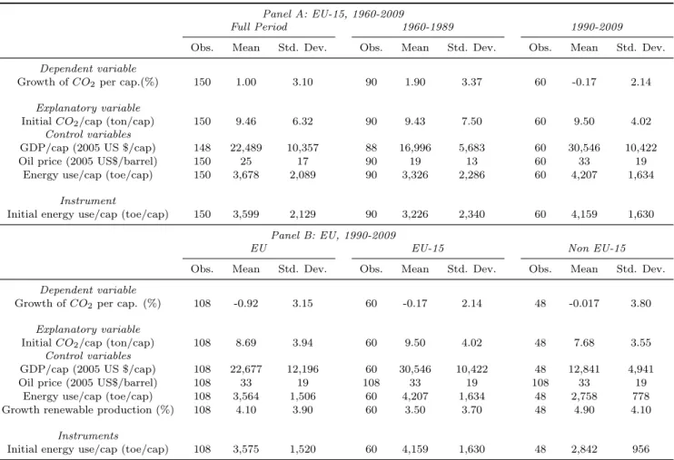
Table 1 below displays the summary statistics for the two panel data sets. Before the
12We tested different instruments for the initial level of per capita emissions like the savings rate and the
population growth rate following economic growth theory (Brock and Taylor,2010). The first stage test reveals that these instruments are weak. The results are available upon request.
13The data base omits carbon emissions caused by deforestation, land-use and land-use changes (LULUCF),
and wood burning for energy; but suitable data on these measures are currently unavailable over the whole pe-riod. Other greenhouse gases like methane, nitrous oxide and fluorinated gases are emitted in smaller quantities than CO2. The most important GHG is by far CO2 which accounts for more than 80% of total EU emissions
1990s, emission growth in EU-15 countries was strictly positive while it became negative after
the 1990s (see panel A, table 1). The examination of the carbon emission growth among all
of the Member States reveals that historical Member States and new Member States both
exhibit a negative emission growth despite their different country characteristics like average
GDP (See panel B, table 1). We must note that the new Member States exhibit lower energy
use per capita and higher growth rates for production of renewable sources than the Historical
Table 1: Summary Statistics
Panel A: EU-15, 1960-2009
Full Period 1960-1989 1990-2009 Obs. Mean Std. Dev. Obs. Mean Std. Dev. Obs. Mean Std. Dev. Dependent variable
Growth of CO2 per cap.(%) 150 1.00 3.10 90 1.90 3.37 60 -0.17 2.14
Explanatory variable
Initial CO2/cap (ton/cap) 150 9.46 6.32 90 9.43 7.50 60 9.50 4.02
Control variables
GDP/cap (2005 US $/cap) 148 22,489 10,357 88 16,996 5,683 60 30,546 10,422 Oil price (2005 US$/barrel) 150 25 17 90 19 13 60 33 19
Energy use/cap (toe/cap) 150 3,678 2,089 90 3,326 2,286 60 4,207 1,634 Instrument
Initial energy use/cap (toe/cap) 150 3,599 2,129 90 3,226 2,340 60 4,159 1,630 Panel B: EU, 1990-2009
EU EU-15 Non EU-15
Obs. Mean Std. Dev. Obs. Mean Std. Dev. Obs. Mean Std. Dev. Dependent variable
Growth of CO2 per cap. (%) 108 -0.92 3.15 60 -0.17 2.14 48 -0.017 3.80
Explanatory variable
Initial CO2/cap (ton/cap) 108 8.69 3.94 60 9.50 4.02 48 7.68 3.55
Control variables
GDP/cap (2005 US $/cap) 108 22,677 12,196 60 30,546 10,422 48 12,841 4,941 Oil price (2005 US$/barrel) 108 33 19 108 33 19 108 33 19
Energy use/cap (toe/cap) 108 3,564 1,506 60 4,207 1,634 48 2,758 778 Growth renewable production (%) 108 4.10 3.90 60 3.50 3.70 48 4.90 4.10
Instruments
Initial energy use/cap (toe/cap) 108 3,575 1,520 60 4,159 1,630 48 2,842 956 Source: Growth of CO2 per cap. and Initial CO2/cap:World Bank(2013); GDP/capHeston et al.(2012); Growth renewable
produc-tion and Energy use/capEUROSTAT(2013). Notes: Cap.emission growth is the average growth rate of per capita emissions over the five-year period; Initial cap. CO2/cap is the level of per capita CO2 emissions at the beginning of each five-year period; GDP/cap is
the average GDP per capita over the five-year period; Energy use/cap is the average energy use per capita over the five-year period; Growth renewable production is the average growth rate of renewable energy supply over the five-year period; Initial Energy use/cap is the level of energy use per capita at the beginning of each five-year period.
4
Results
We first discuss the regression results of equations (2) and (3) to investigate whether CO2
emissions have converged among the EU countries. We then use these results to run bootstrap
simulations to investigate the effect of macroeconomic shocks (or variables) and climate and
energy policy on emission growth.
Conditional convergence in CO2 emissions
Before examining in detail the conditional convergence in emissions, we discuss the results
of the first stage regression of the initial per capita CO2 emissions on the instrument (the initial
per capita energy use for country i ) and the other control variables. The results are reported
in table 2. We immediately notice that the F-First stage statistics is significant across all
specifications.
Table 2: First-stage regressions, equation (2)
(1) (2) Log(initialEner.use/cap) 1.385 1.379 (0.189)∗∗ (0.188)∗∗ Log(GDP/cap) 1.987 -0.160 (2.849) (0.100) Log(GDP/cap) ∗ P ER1 3.265 5.294 (2.987) (1.295)∗∗∗ Log(GDP/cap)2 -0.104 (0.138) Log(GDP/cap)2∗ P ER1 -0.174 -0.273 (0.146) (0.066)∗∗∗ Log(OilP rice) -0.037 -0.038 (0.022)∗ (0.022)∗ Log(Ener.use/cap) -0.493 -0.477 (0.215)∗∗∗ (0.213)∗∗∗ R2 0.986 0.986 F-First Stage 53.95 53.80 Obs 148 148
Notes: First-stage regressions of equation (2) are displayed. Log initial Ener.Use/cap is the log of the energy use per capita at the beginning of period; Log(GDP/cap) is the log of the per capita GDP of country i; Log(GDP/cap)2 is the log of the square of per capita GDP; Log(OilP rice) is the log of the oil price; Log(Ener.use/cap) is the log of the energy use per capita of country i. Tstat are reported in brackets. *,**,*** denote respectively significance at 10%, 5% and 1% level.
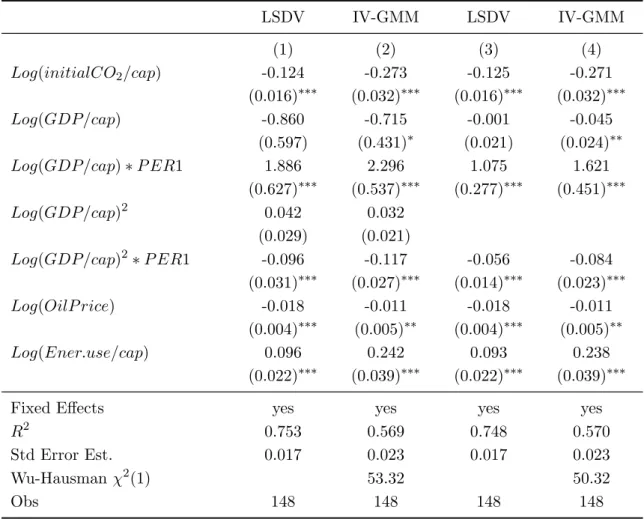
Table 3 presents the regression results using the two methods, LSDV and IV-GMM, for
the EU-15 countries from 1960 to 2009. The coefficient of convergence is significant and robust
across the model specifications implying that the speed of convergence in the EU-15 countries is
0.31.14 This means that EU-15 countries should be at 5% of the asymptotic value of emission in roughly 10 years, i.e., they should stabilize their per capita emissions in roughly 10 years, ceteris
paribus. A structural break in the relation between emission growth and GDP per capita exists.
Before 1990, this relation could be represented by an inverted U-shaped function. The
semi-elasticity of emission growth with respect to GDP per capita is -0.05, meaning that an increase
in one percent in GDP per capita causes a decrease of 0.05 percentage point in emission growth.
Since the mid-1990s, the relation between emission growth and per capita GDP is significantly
negative, the semi-elasticity being equal to −0.04. As expected, any increase by one percent
in oil price causes a decrease of 0.01 point of percentage in emission growth. The energy use
per capita positively impacts emission growth, the semi- elasticity being equal to 0.24. Thus,
any climate policy aiming to promote energy efficiency (or a decrease in energy use per capita)
can contribute to a decrease in emission growth.
Before turning to the analysis of conditional convergence in CO2 among all of the EU
countries from 1990 to 2009, we check the validity of the instruments by analyzing the results of
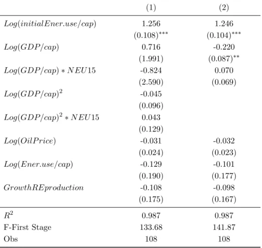
the first-stage regression (see Table 4). The F-First stage is significant across all specifications.
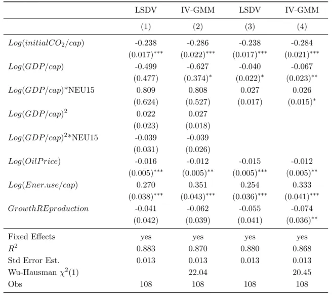
Table5presents the regression results of equation (3) for the EU countries over the period
1990-2009. Despite the inclusion of the new Member States in our sample, the null hypothesis of
conditional convergence cannot be rejected. The convergence speed is robust to the enlargement
of the EU and equal to 0.33 indicating that all EU Member States should be at 5% of the
asymptotic value of emissions in roughly 10 years, i.e., around 2020. This result is in line with
other studies (Jobert et al., 2010). Our analysis reveals that the relation between emission
growth and per capita GDP is statistically different between historical and new Member States.
However, the elasticity of the EU-15 countries (−0.067) is slightly larger than the
semi-elasticity of the new Member States (−0.039). The coefficient associated with oil price is
statistically significant and equal to −0.012. So, we can argue that energy price spikes cannot
14The speed of convergence is calculated as follows: −log(1 + β
1) where β1 is the coefficient of the level of
Table 3: Regressions results. Conditional convergence in CO2 among EU-15 from 1960 to 2009. LSDV IV-GMM LSDV IV-GMM (1) (2) (3) (4) Log(initialCO2/cap) -0.124 -0.273 -0.125 -0.271 (0.016)∗∗∗ (0.032)∗∗∗ (0.016)∗∗∗ (0.032)∗∗∗ Log(GDP/cap) -0.860 -0.715 -0.001 -0.045 (0.597) (0.431)∗ (0.021) (0.024)∗∗ Log(GDP/cap) ∗ P ER1 1.886 2.296 1.075 1.621 (0.627)∗∗∗ (0.537)∗∗∗ (0.277)∗∗∗ (0.451)∗∗∗ Log(GDP/cap)2 0.042 0.032 (0.029) (0.021) Log(GDP/cap)2∗ P ER1 -0.096 -0.117 -0.056 -0.084 (0.031)∗∗∗ (0.027)∗∗∗ (0.014)∗∗∗ (0.023)∗∗∗ Log(OilP rice) -0.018 -0.011 -0.018 -0.011 (0.004)∗∗∗ (0.005)∗∗ (0.004)∗∗∗ (0.005)∗∗ Log(Ener.use/cap) 0.096 0.242 0.093 0.238 (0.022)∗∗∗ (0.039)∗∗∗ (0.022)∗∗∗ (0.039)∗∗∗
Fixed Effects yes yes yes yes
R2 0.753 0.569 0.748 0.570
Std Error Est. 0.017 0.023 0.017 0.023
Wu-Hausman χ2(1) 53.32 50.32
Obs 148 148 148 148
Notes: Regression results of equation (2) are displayed. Tstat are reported in brackets. *,**, and *** denote re-spectively significance t 10%, 5% and 1% level. The initial CO2/cap for country i (expressed in log) is instrumented
Table 4: First-stage regressions, equation (3) (1) (2) Log(initialEner.use/cap) 1.256 1.246 (0.108)∗∗∗ (0.104)∗∗∗ Log(GDP/cap) 0.716 -0.220 (1.991) (0.087)∗∗ Log(GDP/cap) ∗ N EU 15 -0.824 0.070 (2.590) (0.069) Log(GDP/cap)2 -0.045 (0.096) Log(GDP/cap)2∗ N EU 15 0.043 (0.129) Log(OilP rice) -0.031 -0.032 (0.024) (0.023) Log(Ener.use/cap) -0.129 -0.101 (0.190) (0.177) GrowthREproduction -0.108 -0.098 (0.175) (0.167) R2 0.987 0.987 F-First Stage 133.68 141.87 Obs 108 108
Notes: First-stage regressions of equation (3) are displayed. LoginitialEner.U se/cap is the log of the energy use per capita at the beginning of period; Log(GDP/cap) is the log of the per capita GDP of country i; Log(GDP/cap)2 is the log of the square of per capita GDP; Log(OilP rice) is the log of oil price; Log(Ener.use/cap) is the log of the energy use per capita of country i; GrowthREproduction is the average growth rate of the production of renewable sources over each five years period. Tstat are reported in brackets. *,**,*** denote respectively significance at 10%, 5% and 1% level.
result in a substantial decrease in emission growth. However, climate policy especially policy
aiming to promote energy efficiency, can have a higher impact on emission growth. The
semi-elasticity of per capita energy use is quite large and reaches 0.33 while an increase of one point
of percentage in the growth rate of renewable sources production causes a decrease of 0.07
point of percentage in emission growth.
Effectiveness of climate and energy policy
In light of our results, we can discuss the effectiveness of climate and energy policy. From
the analysis of the conditional convergence,we know that the EU countries should succeed in
stabilizing their carbon emissions in roughly ten years. We employ bootstrap method by using
Table 5: Regressions results. Conditional convergence in CO2 among all EU Member States from 1990 to 2009 LSDV IV-GMM LSDV IV-GMM (1) (2) (3) (4) Log(initialCO2/cap) -0.238 -0.286 -0.238 -0.284 (0.017)∗∗∗ (0.022)∗∗∗ (0.017)∗∗∗ (0.021)∗∗∗ Log(GDP/cap) -0.499 -0.627 -0.040 -0.067 (0.477) (0.374)∗ (0.022)∗ (0.023)∗∗ Log(GDP/cap)*NEU15 0.809 0.808 0.027 0.026 (0.624) (0.527) (0.017) (0.015)∗ Log(GDP/cap)2 0.022 0.027 (0.023) (0.018) Log(GDP/cap)2*NEU15 -0.039 -0.039 (0.031) (0.026) Log(OilP rice) -0.016 -0.012 -0.015 -0.012 (0.005)∗∗∗ (0.005)∗∗ (0.005)∗∗∗ (0.005)∗∗ Log(Ener.use/cap) 0.270 0.351 0.254 0.333 (0.038)∗∗∗ (0.043)∗∗∗ (0.036)∗∗∗ (0.041)∗∗∗ GrowthREproduction -0.041 -0.062 -0.055 -0.074 (0.042) (0.039) (0.041) (0.036)∗∗
Fixed Effects yes yes yes yes
R2 0.883 0.870 0.880 0.868
Std Error Est. 0.013 0.013 0.013 0.013
Wu-Hausman χ2(1) 22.04 20.45
Obs 108 108 108 108
Notes: Regression results of equation (3) are displayed. Tstat are reported in brackets. *,**, and *** denote re-spectively significance t 10%, 5% and 1% level. The initial CO2/cap for country i (expressed in log) is instrumented
with the initial energy use per capita of country i (expressed in log).
emissions if nothing else changes (control variables are at their 2005-2009 value).15 The results are named Benchmark Scenario. To examine the efforts that the EU Member States should
make to achieve their targets, we plot figure6which presents the asymptotic value of per capita
emissions as calculated by the bootstrap (presented by the bars in figure 6) and the target for
carbon emissions as defined by the European Commission (the triangles in figure 6).16 The EU Members are classified in descending order of the difference between the carbon emission
target and the asymptotic value of the carbon emissions. We immediately notice that some
new Member States (Estonia, Lithuania, Slovakia, Latvia, Bulgaria, Romania, Czech Republic,
15We run 5,000 iterations. The results are robust if we increase the number of iterations to 10,000. 16
The European Commission has defined the CO2 emission reduction targets as the percentage reduction of
Poland and Hungary) could do even better than initially targeted if they stabilize their carbon
emissions. More surprisingly, Germany, Great-Britain and France belong to this group. Most
of the historical Member States should adopt more aggressive climate policies.
We now analyze how economic factors can affect the efforts that should be made by each
country and how climate and energy policies can help them to meet their country targets (see
figure 5). We define four scenarios: 1)under the Scenario GDP, we employ GDP per capita
forecasts for the period 2020-2024 made by the EIA;17 2) the average oil price rises from US $75 per barrel in 2005-2009 to US$105 in 2020-2024 as projected by EIA (EIA,2014) –Scenario
Oil Price–; 3) the EU countries decrease their energy use per capita by 20% below their 1990
levels–Scenario Energy Use–; 4) the growth rate of renewable production increases by 20% in
all Member States– Scenario Renewable Sources.
Figure 6: Emission target and asymptotic value of carbon emissions under the Benchmark Scenario
Notes: The bar represents the asymptotic value of carbon emissions under the Benchmark Scenario. The triangle represents the country’s specific target.
In table6, we present the difference between each country’s specific target and the
asymp-totic value of carbon emissions as calculated by the bootstrap simulations under the Benchmark
17According toEIA(2014), the annual average growth rate should be equal to 1.06% for EU-OECD Members
Scenario and under each alternative scenario. A positive difference means that the asymptotic
value of carbon emissions is below the target, meaning the country can meet its target by
stabilizing carbon emissions. A negative difference means that the asymptotic value of carbon
emissions is above the target, meaning the country should adopt a more aggressive policy to
reach its target. The higher the difference, the greater the effort the country needs to make.
To investigate which economic factor or which climate policy may help the EU Member States
to meet their target, we compare the results of the Benchmark Scenario with the results of the
four alternative scenarios. We can immediately notice that economic growth does not impact
the efforts that should be made by the EU members. The rise in oil price (or more generally
in fossil fuel price) does not cause substantial decreases in growth emissions, and thus, also
does not impact the asymptotic value of carbon emissions with the exception of Luxemburg,
France and Slovenia. Improvement in energy efficiency and investment in renewable sources
can help EU Members to reach their targets. If Sweden and Luxemburg increase their share of
renewable sources in total energy production, they are on track to meet their targets, ceteris
Table 6: Difference between each country’s specific target and asymptotic value of carbon emissions under the Benchmark Scenario and alternative scenarios (Tons CO2 per capita)
Scenarios
EU Member States Benchmark GDP Oil Price Energy Use Renewable Sources
Estonia 14.18 14.50 14.34 16.82 14.63 Lithuania 7.27 7.53 7.33 8.17 7.42 Slovakia 6.69 6.88 6.78 8.23 6.91 Latvia 5.29 5.50 5.34 6.01 5.44 Bulgaria 4.70 5.08 4.78 6.02 4.99 Romania 4.23 4.23 4.29 5.13 4.42 Czech republic 4.03 4.35 4.19 6.61 4.44 Poland 3.28 3.50 3.39 5.05 3.56 Germany 1.72 2.14 1.85 3.86 2.01 Hungary 1.32 1.48 1.40 2.55 1.48 Great Britain 0.55 0.90 0.66 2.34 0.80 Malta 0.35 0.75 0.43 1.75 0.54 Slovenia 0.08 0.30 0.19 1.89 0.38 France 0.07 0.34 0.15 1.41 0.31 Sweden -0.09 -0.14 -0.02 1.07 0.14 Luxemburg -0.39 0.58 -0.09 4.52 0.57 Belgium -0.64 -0.19 -0.50 1.63 -0.46 Italy -0.94 -0.60 -0.83 0.78 -0.66 Denmark -1.01 -0.61 -0.89 1.00 -0.62 Netherlands -1.07 -0.60 -0.92 1.29 - 0.76 Cyprus -1.37 -0.91 -1.27 0.27 -1.18 Portugal -1.47 -1.20 -1.39 -0.14 -1.27 Austria -1.54 -1.10 -1.42 0.35 -1.19 Greece -1.58 -1.19 -1.46 0.36 -1.20 Spain -1.93 -1.19 -1.84 -0.32 -1.71 Ireland -2.04 -1.61 -1.91 0.07 - 1.83 Finland -2.16 -1.67 - 2.01 0.34 -1.60
Notes: We calculate the difference between each country’s specific target and the asymptotic value of carbon emissions as calculated by the bootstrap simulations. A positive sign means that the country emits less than its carbon target, meaning that the country can meet its target by stabilizing carbon emissions. A negative sign means that the country’s emissions are higher than its carbon target, indicating that the country should adopt a more aggressive policy. Under the Benchmark Scenario, we assume that carbon emissions are stabilized and that the control variables are at their
5
Conclusion
We investigate per capita CO2 emission trends across Member States to examine the
effectiveness of climate and energy policies. We test the assumption of a beta-type convergence
for per capita CO2emissions, conditional upon per capita output, world oil price, energy use per
capita and investment in renewable sources. As predicted by the literature on β-convergence,
we find a decreasing relation between emission growth and the initial level of CO2 per capita.
The EU-15 countries should stabilize their per capita carbon emissions in roughly 10 years,
i.e., 2020. This result holds if we include the new Member States. We also examine how
the country characteristics may affect the convergence process. A decreasing relation between
emission growth and GDP per capita among historical Member States after the 1990s exists.
This result holds if new Member States are included. A shock on fossil fuel price should have
a limited impact on emission growth, ceteris paribus while investment in renewable energy
and in energy efficiency should affect negatively emission growth (see figure 5). By using
bootstrap method, we show that the burden of emission reduction is not shared equally among
the EU countries. Historical Member States like Germany, Great-Britain and France can hit
their carbon target without increasing their investments in green technologies or improving
their energy efficiency. Other historical Member States should invest in more energy efficient
technologies to reach their domestic targets (e.g. their carbon emissions will be below the
targeted levels). The new Member States are expected to be well below their domestic targets
even if there is an increase in per capita income or in oil price.
Our findings have important implications for EU climate policy. Since most of the EU
countries must make substantial efforts to reach the 2020 target, the 2030 target of 40%
re-duction seems to be out of reach without quite substantial investment in renewable technology
and energy efficiency. But, investment in green technologies seems to have slowed down. The
sovereign debt crisis in Europe has crimped funding for green projects and investment in energy
efficiency. The rise of technologies tapping cheap unconventional resources like shale gas and
shale oil has caused the recent decline of crude oil price and has dented prospects for renewable
technologies. After the Fukushima nuclear disaster, some countries like Germany have stepped
References
Arellano, M. and Bond, S. (1991). Some tests of specification for panel data: Monte carlo
evidence and an application to employment equations. The Review of Economic Studies,
58(2):277–297.
Arellano, M. and Bover, O. (1995). Another look at the instrumental variable estimation of
error-components models. Journal of Econometrics, 68(1):29–51.
Barro, R. J. and Sala-i Martin, X. (1992). Convergence. Journal of Political Economy,
100(2):223–251.
Baumol, W. J. (1986). Productivity Growth, Convergence, and Welfare: What the Long-Run
Data Show. The American Economic Review, 76(5):1072–1085.
Brock, W. A. and Taylor, M. S. (2010). The Green Solow Model. Journal of Economic Growth,
15(2):127–153.
Checherita-Westphal, C. and Rother, P. (2012). The impact of high government debt on
economic growth and its channels: An empirical investigation for the euro area. European
Economic Review, 56(7):1392–1405.
Directive 2012, E. (2012). Directive 2012/27/CE of the European Parliament and of the Council
of 25 October 2012 on energy efficiency, amending Directives 2009/125/EC and 2010/30/EC
and repealing Directives 2004/8/EC and 2006/32/EC. Official Journal of the European
Communities L, 315.
Durlauf, S. N., Johnson, P. A., and Temple, J. R. (2005). Growth econometrics. Handbook of
Economic Growth, 1:555–677.
Eboli, F. and Davide, M. (2012). The EU and Kyoto Protocol: Achievements and Future
Challenges. Review of Environment, Energy and Economics (Re3), FEEM Working Paper.
EEA (2013a). Annual European Union greenhouse gas inventory 1990-2011 and inventory
EEA (2013b). Trends and projections in Europe 2013: Tracking progress towards Europe’s
energy and climate targets until 2020. European Environment Agency.
EIA (2014). Analysis and Projections: International Projections to 2040. Energy Information
Administration.
European Council (2014). Conclusions on Climate and Energy Policy Framework. Note,
Brussels, 23 October 2014.
EUROSTAT (2013). Data Base. European Commission.
Greene, W. H. (2012). Econometric Analysis, Seventh Edition. Prentice Hall.
Heston, A., Summers, R., and Aten, B. (2012). Penn World Table Version 7.1. Center for
International Comparisons of Production, Income and Prices at the University of
Pennsyl-vania.
IEA (2013). Energy Efficiency Market Report 2013: Market Trends and Medium-Term
Prospects. International Energy Agency.
Jobert, T., Karanfil, F., and Tykhonenko, A. (2010). Convergence of per capita carbon dioxide
emissions in the EU: Legend or reality? Energy Economics, 32(6):1364–1373.
Keppler, J. H. (2007). L’Union Europ´eenne et sa politique ´energ´etique. Politique ´etrang`ere,
3:529–543.
Ord´as Criado, C. and Grether, J.-M. (2011). Convergence in per capita CO2 emissions: A
robust distributional approach. Resource and Energy Economics, 33(3):637–665.
Ord´as Criado, C., Valente, S., and Stengos, T. (2011). Growth and pollution convergence:
Theory and evidence. Journal of Environmental Economics and Management, 62(2):199–
214.
Quah, D. T. (1996). Empirics for economic growth and convergence. European Economic
Strazicich, M. C. and List, J. A. (2003). Are CO2 emission levels converging among industrial
countries? Environmental and Resource Economics, 24(3):263–271.
World Bank (2013). Data Base. World Bank.
World Bank (2014). World Bank Commodity Price Data Pink Sheet. World Bank.
Zugravu, N., Millock, K., and Duchene, G. (2010). Les facteurs de la d´epollution dans les pays