City size distribution in China: are large cities dominant?

Texte intégral

(1)2014s-04. City size distribution in China: are large cities dominant? Zelai Xu, Nong Zhu. Série Scientifique Scientific Series. Montréal Janvier/January 2014. © 2014 Zelai Xu, Nong Zhu. Tous droits réservés. All rights reserved. Reproduction partielle permise avec citation du document source, incluant la notice ©. Short sections may be quoted without explicit permission, if full credit, including © notice, is given to the source..

(2) CIRANO Le CIRANO est un organisme sans but lucratif constitué en vertu de la Loi des compagnies du Québec. Le financement de son infrastructure et de ses activités de recherche provient des cotisations de ses organisations-membres, d’une subvention d’infrastructure du Ministère de l'Enseignement supérieur, de la Recherche, de la Science et de la Technologie, de même que des subventions et mandats obtenus par ses équipes de recherche. CIRANO is a private non-profit organization incorporated under the Québec Companies Act. Its infrastructure and research activities are funded through fees paid by member organizations, an infrastructure grant from the Ministère de l'Enseignement supérieur, de la Recherche, de la Science et de la Technologie, and grants and research mandates obtained by its research teams. Les partenaires du CIRANO Partenaire majeur Ministère de l'Enseignement supérieur, de la Recherche, de la Science et de la Technologie Partenaires corporatifs Autorité des marchés financiers Banque de développement du Canada Banque du Canada Banque Laurentienne du Canada Banque Nationale du Canada Banque Scotia Bell Canada BMO Groupe financier Caisse de dépôt et placement du Québec Fédération des caisses Desjardins du Québec Financière Sun Life, Québec Gaz Métro Hydro-Québec Industrie Canada Investissements PSP Ministère des Finances et de l’Économie Power Corporation du Canada Rio Tinto Alcan State Street Global Advisors Transat A.T. Ville de Montréal Partenaires universitaires École Polytechnique de Montréal École de technologie supérieure (ÉTS) HEC Montréal Institut national de la recherche scientifique (INRS) McGill University Université Concordia Université de Montréal Université de Sherbrooke Université du Québec Université du Québec à Montréal Université Laval Le CIRANO collabore avec de nombreux centres et chaires de recherche universitaires dont on peut consulter la liste sur son site web. Les cahiers de la série scientifique (CS) visent à rendre accessibles des résultats de recherche effectuée au CIRANO afin de susciter échanges et commentaires. Ces cahiers sont écrits dans le style des publications scientifiques. Les idées et les opinions émises sont sous l’unique responsabilité des auteurs et ne représentent pas nécessairement les positions du CIRANO ou de ses partenaires. This paper presents research carried out at CIRANO and aims at encouraging discussion and comment. The observations and viewpoints expressed are the sole responsibility of the authors. They do not necessarily represent positions of CIRANO or its partners.. ISSN 2292-0838 (en ligne). Partenaire financier.

(3) City size distribution in China: are large cities dominant?. *. Zelai Xu †, Nong Zhu ‡. Résumé/abstract This paper examines the evolution in size distribution of Chinese cities. Since the relaxation of restrictions on rural/urban migration in the 1980s, China has experienced rapid urban growth. However, cities of different sizes have experienced varying patterns of growth. We first describe the evolution of city size distribution in China by documenting the growth both of city size and of the number of existing cities. Then, focusing on the period from 1990-2000, we characterize the urban evolution trend with the Pareto law estimation, and examine the mobility of cities between different size groups with the Markov transition matrix. We also test the convergence hypothesis in the city population growth process. Our results suggest that, contrary to the expected dominance of large cities’ growth, Chinese city size distribution evened out over the 1990s, with small cities growing more rapidly than large cities. Mots clés/keywords : City size distribution, Zipf’s law, Convergence, China.. *. This article was published in Urban Studies, vol.46, no.10, p. 2159-2185. CERDI-IDREC, Université d’Auvergne, France ‡ INRS-UCS, University of Quebec. Corresponding author: INRS-UCS, 385 rue Sherbrooke Est, Montreal, QC, H2X 1E3, Canada. Tel: 1-514-499-8281. Fax.: 1-514-499-4065. Nong.Zhu@UCS.INRS.Ca †.

(4) 1. Introduction Since the late 1970s, China’s urban population has grown rapidly, in contrast with a decline in the country’s overall population growth due to its demographic control policy. As a result, the urban population increased from 17.92% of the total population in 1978 to 42.99% in 2005 (NSB, 2006). With an average annual growth rate higher than 4% for over nearly three decades, Chinese urban growth ranks among the most rapid in the world. More than half of the Chinese population is expected to live in cities and towns by the year 2020 (United Nations, 2004). This trend of recent rapid urban growth contrasts sharply with the slow or even stagnant urbanisation process observed during the 1960s and 1970s. At that time, the government control on population mobility, in particular on migration from rural areas to cities, deprived farmers of the freedom to seek employment in urban areas. In the 1980s, with the progress of economic reforms, restrictions on migration were loosened. As a result, during that decade, the urban population grew by more than 100 million, most of which was attributed to rural-urban migration flow (Chang, 1994). Urban growth usually takes two forms: the expansion of existing urban settlements, and the formation of new ones. The rapid urbanization process which took place in China resulted in a considerable increase in the number of Chinese cities. In 1978, China had only 193 cities. The number increased to 434 in 1988 and 657 in 2005 (NSB, 2006). Most existing cities also expanded considerably, in terms of both surface area and inhabitant numbers. A feature of urban growth that is worthy of notice is that large and small cities do not grow in the same way, which leads to the evolution of city size distribution. This issue has attracted considerable attention in urban economics literature; it is argued that agglomeration economies exist, associated with city size. This means that large cities have productivity advantage over small cities1. However, based on development strategies and political ideologies, city size growth in China was strictly controlled at least since the 1960s; in particular, the growth of large cities was greatly restricted. Hence, in the pre-reform era, the city size distribution pattern was the direct outcome of central government policies, and urban population grew mainly through the creation of new urban unities and the development of small and medium sized cities. During the post-reform period, with the gradual relaxation of restrictions on migration, the rural population spread to urban areas. In the meantime, as the market mechanism was introduced into the urban economy, cities rid themselves of many administrative constraints and regained autonomy over their growth. It is believed that the urban growth process in China is increasingly subject to interactions between market actors rather than state planning. Undoubtedly, this transition in the Chinese urban system has led to accelerating urban growth. However, little is known about the recent urban growth pattern. Do cities of different sizes grow at the same rate? Or are there specific types of cities that grow more rapidly than others? This paper aims to examine city size distribution changes in the recent Chinese urban transition. Since large cities are believed to have productivity advantages, we hypothesized that, in contrast to the pre-reform pattern, the growth of large cities has recently accelerated to become the main source of urban growth. Thus, the specific objective of this study was to investigate whether there have been any changes in city size distribution favouring large cities during the decade of the 1990s. Most empirical works on city size distribution are devoted to developed economies; to our knowledge, only two recent studies are devoted to China (Song and Zhang, 2002; Anderson and Ge, 2005). This paper examines the evolutionary trend of Chinese cities during the 1990s in terms of size distribution, by using different approaches of analysis. In Section 2, we provide an overview of the Chinese urban system. Section 3 then gives a general review of city size distribution since 1949. In Section 4, we examine the evolution of city size distribution during the 1990s using various approaches. Finally, Section 5 provides some concluding remarks.. 1. There exists a voluminous body of literature providing theoretical foundation and empirical tests for the existence of agglomeration economies. See Eberts and McMillen (1999), and Rosenthal and Strange (2004) for a comprehensive review. Recently, Au and Henderson (2006) argued that the majority of Chinese cities are undersized, which results in large losses in GDP..

(5) 2. Overview of the Chinese urban system 2.1. Chinese cities By the end of the year 2004, there were 661 cities in China, with a total population of 341.47 million people, or 62.9% of the total urban population (NSB, 2005). Each city had an average of 517 000 inhabitants. The rest of the urban population was distributed within 19 883 towns, which had an average population size of 10100 inhabitants. Among the 661 cities, there were 497 cities with less than 500 000 inhabitants. These cities represented 75.2% of the total number of cities, but only 29.6% of the total city population. At the other end of the urban hierarchy, 28 large cities with more than 2 million inhabitants accounted for 34.3% of the total city population, and among others, the 7 largest cities with more than 5 million inhabitants accommodated 16.2% of the total city population (calculated from CMC, 2006). In the Chinese urban system, there are three levels of cities: cities under direct administration of the central government (zhi xia shi); cities at the prefecture level administered by provinces (di ji shi); and cities at the county level administered by prefectures or provinces (xian ji shi)2. In 2003, there were 4 province-level cities, 282 prefecture-level cities and 374 county-level cities. 2.2. City population measure Studies on Chinese urban issues often encounter difficulties in finding an appropriate and coherent measure of the urban population. These difficulties stem from the frequent changes in urban area definition and the various statistics of the urban population in China. Our data is compiled from Fifty Years of Chinese City Development and Chinese City Statistical Yearbook (NSB, several issues). City population is measured based on the “non-agricultural population” statistic in the following analyses if not explicitly noted. Our choice is to a great extent constrained by data availability, since Fifty Years of Chinese City Development only provides non-agricultural population distribution by four size groups of all cities from 1949 to 1998, and the 1991-2001 editions of Chinese City Statistical Yearbook only report a non-agricultural population indicator for all cities. This choice has some advantages over other measures of urban population; nevertheless, we recognize that it is not a completely accurate measure of the urban population in China. According to international practice, an urban population includes two components: a majority of inhabitants in the central urban area, and an additional constituent in nearby suburbs. Therefore, an appropriate urban population measure should follow the residential place principle, and be based upon an accurate definition of urban areas. Unfortunately, China did not have such a measure of its urban population until at least the year 1990. There are mainly two statistics officially published as measures of the urban population before 1990, namely the total city and town population (TCTP), and the nonagricultural population (NAP). Neither accurately reflects the actual urban population. The former counted all people under the administrative area of cities and towns, the latter only considered people having non agricultural Hukou status. Hukou was a special household register system administered by the Ministry of public security, which came into force in the 1950s. Theoretically, the definition of the urban population should have been straightforward with a population register system; however, the Hukou system was not merely a simple system of population register, but was attributed special functions under the planned economy regime. The Hukou system divided people into agricultural and non-agricultural categories rather than rural and urban categories. Non-agricultural Hukou status yielded access to a set of privileges, including food rations, low rent housing, education, job allocations, a social security system, etc. During the pre-reform period, the non-agricultural population was not very different from the urban population, since initially, most of the urban inhabitants had been attributed non-agricultural Hukou status. However, with the progress of economic reforms, more 2. Informally, there is an intermediate level between province-level cities and prefecture-level, called quasiprovince level. Most of the vice-province level cities are capitals of provinces. Since the distinction of this level is to a great extent related to the administrative hierarchy, we consider these cities as prefecture-level cities in our analysis.. 2.

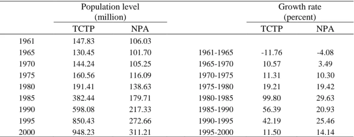
(6) and more of the rural population entered urban areas, either due to the expansion of urban areas or through migration, yet only some of them acquired non-agricultural Hukou status. Therefore, the nonagricultural population measure increasingly under-estimated the actual urban population. The reason why the NAP indicator is preferred over TCTP by some authors (Wu, 1994; Song and Zhang, 2002) and even by official statistical authorities is that it remained unaffected or only slightly affected by urban area definition changes. While the TCTP measure changed significantly and included an excessive share of the agricultural population during periods of loose urban area definition 3 , the NPA measure remained quite coherent. The evolution of the two indicators is illustrated in Table 1, where we observe that the TCTP number tripled dramatically from 1980 to 1990, a decade in which the definition of urban area was expanded to include vast suburb areas, while variations of the NPA indicator are quite stable. 2.3. Urban growth from 1949-2000 The introduction of economic reforms in China in 1978 can be viewed as a turning point, on which a comparative analysis of urbanization and the urban growth process in China can be based (see Figure 1). In the pre-reform period, the non-agricultural population of cities rose from 27.40 million in 1949 to 79.87 million in 1978 with an average annual growth rate of 4.20%, and the number of cities increased from 132 to 193, with an average of 2.1 cities created each year. The average city size doubled from 208 000 to 414 000 inhabitants. In the post-reform period, the non-agricultural population of cities increased to 231.27 million in 2000, with an annual growth rate of 4.69%. The number of cities rose to 664, with an average annual creation of 20.4 new cities. The average city size shrank to 361 000 inhabitants. Cities are usually classified into four size groups in China (see Table 2). In terms of the population distribution among these size groups, in 1978, 153 cities with fewer than 500 000 inhabitants (the two smallest size groups) and 13 cities with more than 1 million inhabitants both represented 37.5% of the total population. In 2000, there were 570 cities with fewer than 500 000 inhabitants, which accommodated 46.7% of the total city non-agricultural population, and the 42 largest cities with more than 1 million inhabitants represented 37.5% of the city population. A comparison of these two phases reveals distinct urban evolution trends before and after 1978, although the city population grew at about the same rate during both of these time periods. Many more cities were created in the post-reform period. The growth of the urban population before 1978 stemmed mainly from the expansion of pre-existing cities, while after 1978, it depended largely on the creation of new cities. A large number of small cities was created in the post-reform period, which led to an increase in the number of people dwelling in smaller cities, and the shrinking of the overall average city size. This finding is contrary to our expectations, as we anticipated finding evidence of rapid growth of large cities during the reform period. However, given that urban growth trends do not remain stable over long periods of time, we must further examine fluctuations within each of the two periods. The pre-reform period can be further divided into two stages: 1) The rapid growth stage from 1949 to 1958. This period witnessed the most rapid growth of the urban population. 52 new cities were created in nine years and the average annual growth rate of the non-agricultural population was over 10%. During this period, 91.1% of the urban non-agricultural population growth took place in cities with more than 200 000 inhabitants, which experienced rapid growth, both in terms of the expansion of city size and the increase in the number of cities. The average city size grew from 207 619 to 329 714, namely an increase of 58.8%. 2) The stagnation period of 1959-1978, when city population and numbers increased only slightly, and the number of small cities decreased. It can be seen that the urban population growth prior to economic reforms took place mainly during the 1950s, during the free migration and rapid urbanisation period at the beginning of the new republic. Urban policies changed over the next two decades by implementing restrictions on migration and city size control. As a result, urban growth slowed down, or even stagnated, in terms of both population and city number. 3. This is particularly the case of the 1980s, for example, using the TCTP measure, the official statistical yearbook of 1990 estimated that the urban population in 1989 was 573.83 million and that the urbanization level was 51.5%, which was corrected in statistical publications after 1992 to 295.4 million and 30.7%, respectively.. 3.

(7) The post-reform period can be divided into three stages: The first is from 1979-1989, during which rapid urban growth resumed. On average, 26.7 new settlements entered into the city system and city population grew by 5.7% each year. Of the total increment of city population, 48.9% was contributed by the largest size group of more than 1 000 000 inhabitants, and 31.9% by the smallest size group of fewer than 200 000 inhabitants. Among the four groups, the smallest size group of cities grew most rapidly with the number of cities increasing from 93 to 276 and an annual population growth of approximately 10%. In the single year of 1988, this group gained 43 new cities and a population increase of 20.3%. New cities created during this period were typically small cities, since the average size of this group was only 111 410 inhabitants in 1989. At the top of the urban hierarchy, the largest sized city group also grew considerably , with the number of cities doubling from 15 to 30. The rapid growth at both ends of the urban system was attributed to the significant changes in city definition and reclassification during the 1980s. The loosening of city qualification criteria and the upgrading of districts to district level cites led to an increase in the number of small cities but a decrease in average city size. However, the incorporation of some suburban districts into prefecture level cities resulted in the considerable growth of large cities. The second phase of the post-reform urban growth period was from 1990 to 1995, where city population continued to grow at the high rate of 5.4%. The number of cities increased at a slightly slower rate with 15 new cities created each year. The growth of the largest city size group slowed down, with the addition of only one city, and the population growth rate lower than average. The two smallest city size groups continued to grow rapidly, thanks to the continuous increase in the number of cities. 99 new cities entered the smallest size group, and 76 new cities entered the group of 20 00 000 to 500 000 over these five years, which led to 31.2% and 58.4% of population growth respectively within the two groups. As a result, 63.4% of the growth of the total city population during this stage came from the increment of people living in cities with fewer than 500 000 inhabitants. The overall average city size continued to shrink, reaching 31 285 in 1995. The last stage, from 1996 to 2001, witnessed a decline in city population growth, with an annual growth rate of 3.22%. Population growth in the largest size group represented 58.6% of the growth in the total city population. The growth primarily took the form of city size expansion rather than an increase in the number of cities. In fact, the total city number remained quite stable. The number of cities in each size group increased slightly, except in the smallest one. This implies that cities in all groups expanded in population size and consequently many cities moved up to larger size groups. The average city population rose from 312 000 in 1995 to 360 870 in 2001. The two largest size groups experienced the most rapid growth, both in the number of cities and in population, suggesting that a large number of small and medium-sized cities expanded during this period to become medium-sized and large cities, respectively. In summary, city population grew continuously, without significant fluctuation, during the postreform period. During the first fifteen years, urban growth depended mainly on an increase in the number of cities while the average city size decreased. This was followed by a period during which the expansion of city size became the main source of the urban growth. It is also of interest to look at the evolution of the population share within each city size group. During the pre-reform period, 1) the largest size group maintained a high growth rate during the decade following 1949, both in terms of the number of cities and of population, until it peaked to represent 45% of the total city population in 1964. After that, the percentage began to drop and rejoined the 1949 level, namely 37% of the total city population, on the eve of economic reforms. 2) The two middle groups experienced moderate growth, with the share of cities having 500 000 to 1 000 000 inhabitants rising from 19% in 1949 to 25% in 1978, and that of the second smallest-size group growing from 20% to 23%. 3) The smallest size group was the only group that declined in terms of population share. In sum, the first fifteen years of this period (1949 to 1964) witnessed the rapid growth of the largest size group and the decline of the smallest size group in terms of population share; after 1964, the largest size group began to decline and the two middle groups expanded, which reflects the changes in urban policies after 1964 controlling the expansion of large cities. From the 1980s, 1) with the rapid increase of city numbers in the largest size group, the share of this group in the total population at first followed the ascending tendency to reach the peak of 42% in 1989, then dropped to 35% in 1997, and rose again to 39% in 2001. 2) In contrast, the second largest size group’s share continued to decline. This may be explained by the fact that many cities in the second. 4.

(8) size group expanded in population size and crossed the threshold of 1 000 000 to move into the largest size group. 3) The proportion of population in the two smallest size groups continued to increase at high rates. The share of the smallest size group augmented from 13% in 1980 to 22% in 1994, and in the same year, the total share of these two groups increased to represent approximately half of the total city population. After 1995, city number and population of these two groups stopped growing, which led to a decrease of their shares and the increase of that of the two largest size groups. By placing the facts described above within the historical and political context of the Chinese urbanization process, several features of city population growth can be observed: 1) The rapid growth of city population corresponded to the short free migration period in the 1950s. In particular, the dramatic increase of the population share of the largest-size group in total city population shows the great growth potential and capacity of absorption of large cities under free migration conditions. 2) The slow or even stagnant urban growth in the 1960s and 1970s could be attributed to both the general difficulties encountered by the national economy, and the urban policies controlling the growth of city number and population. 3) The 1980s witnessed a return of rapid urban growth, resulting partly from the loosening of the restrictions on rural/urban migration. However, unlike the growth of the 1950s, urban population and city number growth in this period was largely an outcome of the readjustment and relaxation of the city criterion. A large number of districts were qualified as cities; meanwhile, prefecture level cities expanded their size by enclosing suburban districts. The urban growth of the 1980s can be characterized as government-driven growth. 4) On the contrary, the 1990s corresponded to a period of urbanisation increasingly driven by economic forces. The city definitions were adjusted to be more reasonable and conformed to international practice. The fairly steady city population growth stemmed from the size expansion of pre-existing cities rather than an increase in city number. This was the period in which the market mechanism began to play a dominant role in the economy, and the national economy grew at a relative steady rate, urban population growth resulted primarily from rational decisions of economic agents, namely location choice of individuals and firms. Therefore, in the next section, we focus our study of city size distribution on the period 1990-2000.. 3. The evolution of city size distribution 1990-2000 This section studies Chinese urban system evolution, namely the change of city size distribution and the mobility of cities inside the distribution, during the 1990s. This period is not long enough for the examination of long term trends, however, since the 1980s, China has experienced unprecedented rapid economic growth. A profound transition has involved all domains of China, and the urban sector has undergone great changes during this period as well. 3.1. An overview Over the period from 1990-2000, the total population of China rose from 1143.33 to 1267.43 million, or an increase of 10.85%, while the urban population rose by 50.03% from 301.95 million to 459.06 million. As a result, the urban population rose from 26.41% to 36.22%. As shown in Table 3,196 cities were created during the period 1990-2000; in terms of city size growth, while the overall minimum and maximum city sizes increased by 377.4% and 25.2%, respectively, the average size only increased slightly by 7.8%, which implies that most cities created during 1990-2000 are small. Spatially, most cities were distributed in eastern regions, while western regions had fewer cities. Meanwhile, the average city size diminished from east to west. Standard deviations of city size show that middle and western cities were more evenly distributed than cities in the east. In fact, 114 of the 196 cities created during this decade are located in the east of China, which led to a decrease in average size of eastern cities. In contrast, the average size of middle and western cities increased, as a result, the disparity in terms of average city size among these regions were reduced. The evolution of the city size distribution over time can be examined with non-parametric kernel density estimates. Figure 2 illustrates the shape of the relative city size distributions for 1990 and 2000, based on Epanechnikov Kernel estimates with sizes normalized by the average city size of the year. The relative distributions of the two years appear to be quite similar. Both are uni-modal, with relative sizes concentrated at approximately the same values. However, the degree of concentration is different: 5.

(9) the distribution for 2000 loses density in the left and right tails and gains density in the middle relative to 1990. This suggests that the relative city sizes are more concentrated at average values in 2 000 than in 1990, in other words, they are more evenly distributed. 3.2. Pareto law analysis It was first suggested by a German geographer Auerbach in 1913 (in Gabaix, 1999) that the size distribution of cities in a given territory follows a Pareto distribution as: (1) y  AS  where S is a particular city population size, y is the number of cities with populations no less than S, A and α are positive constants, α is called the power exponent, or Pareto exponent. Sine then, the Pareto law of city size distribution has attracted considerable interest within the field of spatial economics. It is considered one of the most striking regularities in economics4 (Krugman, 1996; Fujita et al, 1999). The original proposition of Auerbach was further developed by Zipf (1949), who stated that the size distribution of cities not only follows the Pareto distribution, but also takes a Pareto exponent equal to 1. The term of “Zipf’s law” frequently employed refers therefore to a special form of the Pareto law where α=1, and the constant A equals the population size of the largest city in the distribution. Empirically, cities of a country are ranked by size in decreasing order, with the largest city numbered 1, and the smallest rank equal to the total number of cities. According to Zipf’s law, the size of a city i noted Ni, is proportional to the reciprocal of it’s rank, or Ni  A / Ri . In other words, the product of a city’s rank and population size is a constant equal to the population of the largest city in the country. This interpretation of the Zipf’s law describes the relationship between size and rank of the cities; it is therefore referred to as the rank-size law. Numerous studies apply the Pareto law in city size distribution analyses. The most often used estimation method is based upon the following regression: ln Rit  ln At  t ln Nit  uit (2) where Rit and Nit indicate respectively the rank and population size of city i at the period t, uit the error term. The Pareto law holds for city data if the log linear regression has a good fitness and the Zipf’s law is obtained for α =1 (or the Pareto exponent is not statistically different from one). If city size distribution follows Pareto law, the Pareto exponent α measures the degree of population concentration in cities of an urban system. Since α is the slope of the log linear regression, a larger α indicates a steeper rank-size line, which implies that the cities of the same rank get smaller in size, given the intercept unchanged; in other words, there is a lower degree of urban concentration, or a more even city size distribution. Thus, an estimate of the Pareto exponent provides a simple way to evaluate the evenness of city size distribution, which can be used to make cross-country or temporal comparisons. A larger value of the Pareto exponent indicates in general a more even population distribution in cities of an urban system. Most empirical works find that the Pareto law regression fits city size distribution quite accurately. For example, Rosen and Resnick (1980) found that 36 out of 44 sample countries had a Parento law regression R2 value higher than 0:95. Using data on French cities from 1831 to 1982, Guérin-Pace (1995) discovered that R2 values were always higher than 0.99 with a threshold of 2000 inhabitants. Contrasted to the regularity of high R2 values in such studies, the estimate of the Pareto exponent shows more variation. Rosen and Resnick (1980) found estimates of α ranging from 0.81 to 1.96 (Australia), with a sample mean of 1.14. Nitsch (2005) made a synthesis of 515 estimates from 29 studies and found that the value of α ranged from 0.49 to 1.96, with a mean of 1.09. Based on Monte Carlo simulations, Gabaix and Ioannides (2004) stated that a value in a range [0.8, 1.2] of the 4. This empirical regularity in city size distribution has however no systematic theoretical foundation. Both traditional models of urban economics (Henderson, 1988) and theories in geography economics (Fujita et al, 1999) are able to explain the existence of cities of different sizes, but neither can predict the city size distribution following Pareto law. Recent work is making efforts to construct theoretic models giving out Pareto law (see Gabaix and Ioannides, 2003). However, a recent work of Gan et al (2006) proves the Zipf’s law’s good fit to be a statistical phenomenon, and it does not require any basis in economic theory.. 6.

(10) exponent may indicate the success of Zipf law. It is widely believed that the estimated value of the Pareto exponent is sensitive to the sample selection criteria. In cross-country studies, Rosen and Resnick (1980) found that the Pareto exponent is larger for more populous countries. Among single country studies, Guérin-Pace (1995) showed that the evolution of the Pareto exponent of France over time followed an inverse U shaped curve. Even for city distribution of a country over the same period, estimates of the Pareto exponent may differ as city population definitions and sample threshold change. Based on US data, Soo (2005) found that Pareto exponent estimates tend to be smaller for urban agglomerations (metropolitan areas) than for city proper data. Moreover, Pareto exponent estimates tend to be larger when studies consider only the upper tail distribution of city size (Black and Henderson, 2003). Most single country studies focus on developed economies, especially the US5, mainly due to the availability of city data. Only a few recent studies investigate Chinese city size distribution. Song and Zhang (2002) used Chinese city data from two years: 1991 and 1998, to estimate Zipf’s law regression. Anderson and Ge (2005) extended the sample to seven years selected from 1949 to 1999. We applied the Pareto law estimation to Chinese city size distribution during the 1990s, in order to examine its evolution during this rapid urban growth period. We used city data from five years selected from 1990 to 2000, namely 1990, 1993, 1995, 1998 and 2000. Results are presented in Table 4. The top panel of Table 4a presents the full sample estimation results: all cities with available population data are included in regressions. The R2 value increases from 0.886 for 1990 to 0.927 for 2000, suggesting that the Pareto law regression increasingly fits Chinese city size distribution throughout this period. However, we note that recently, Gan et al (2006) prove that a good fit of the Pareto law is only a statistical phenomenon, and does not have much economic significance. The estimates of the Pareto parameter show a monotone ascending trend from 1990 to 2000, with values not significantly different from 1 for the first two years, and higher than 1 for the following three years. These results suggest that at the beginning of the 1990s, city size distribution followed Zipf’s law, but has become more equal than predicted by the Zipf’s law in the second half of the decade. As showed in Figure 3, the rank-size line (apart from shifting upwards) rotated clockwise from 1990 to 2000, which suggests decreasing urban concentration, since cities at the top of the hierarchy have smaller relative size than before. The number of cities augmented from 467 in 1990 to 663 in 2000, due to the large number of new cities that entered into the sample during this decade, although a few cities also dropped out. These sample changes may have influenced the overall pattern of city size distribution. In order to account for this influence, we re-estimated the equation for a balanced panel data sample: only cities existing in all five years were included in the sample. Results are presented in middle panel of Table 4a. The Pareto parameter still shows an increasing trend, but the values are slightly smaller than in the complete sample: they are significantly below 1 for the first three years, and not significantly different from 1 for the last two years. This finding implies that existing cities become more evenly distributed over time, and the entry of new cities further augmented the evenness of the full sample city size distribution. According to the Chinese official urban criteria adopted in 1983, agglomerations should have at least 80 000 non-agricultural inhabitants to be qualified as cities. However, not all cities in our sample fit this criterion, since many agglomerations with fewer than 80 000 inhabitants are defined as cities due to their political or administrative importance. We excluded these small cities by employing the threshold of 80 000 inhabitants, which reduced our sample size to between 61(in 2000) and 87 (in 1995) cites. Results are presented in the lowest panel of Table 4a. The Pareto parameter is significantly above 1 for all five years, and the general trend increases consistently. It appears that the exclusion of small cities resulted in a more even city size distribution, better fitted to the Pareto law. This finding also suggests that the estimate of the Pareto exponent is sensitive to the sample threshold. To test this sensitivity further, we ran regressions on the 100, 200, 300 and 400 top cities, respectively. The results presented in Table 4b show that, as suggested by the literature, the more we 5. A series of works estimate the Zipf law regression using the same urban data base of the US over 1900-1990, see Dobkins and Ioannides (2000), Ioannides and Overman (2001), Black and Henderson (2003) Gabaix and Ioannides (2003), Soo (2005).. 7.

(11) move up towards the top of the urban hierarchy, the higher the value of the Pareto exponent is, which implies that larger cities are more evenly distributed than smaller ones. The increasing trend of the Pareto parameter does not change. Recently, Gabaix and Ibragimov (2006) argued that the conventional OLS estimate of the Pareto exponent based on model (2) is biased. They proposed a simple remedy for this bias, which was to use a shift of 1/2 for the rank, and run the regression as follows: (3) ln(Rit  1/ 2)  ln At   t ln Nit  uit We replicated our regressions following this corrected version of OLS Pareto law model, and found that all estimates of the Pareto exponent were larger than with the standard method (see column 2 of Table 4a, results for other regressions are not reported), with a difference of between 0.01 and 0.02. However, the increasing trend of the Pareto exponent from 1990 to 2000 remained unaltered. The fact that the Pareto parameter gets higher as we limit the sample to larger cities suggests that the relationship between rank and size may not be exactly log-linear. We can also observe in Figure 3 that the plot of rank against size in logs are of inverse-U rather than linear shape. We hence add the quadratic term of population size in log to equation (2) as ln Rit  ln At  t ln Nit  t (ln Nit ) 2  uit (4) Estimation results based on equation (4) are presented in the right-hand part of Table 4a for different samples. These confirm the non-linearity in the regression for all samples. The positive coefficient of the log city size term and the negative coefficient of its quadratic term implicate a concave regression line, just as the data plots show. The concavity of the regression line is consistent with the previous finding that the Pareto exponent estimated tends to be larger when we limit the sample to the largest cities. As mentioned above, the rise in Pareto exponent as the sample is limited to top cities is a common finding in the literature. The inverse-U shaped relationship between rank and size in logs is also found in Black and Henderson (2003) for US cities and in Song and Zhang (2002) for Chinese cities. We then ran regressions by distinguishing cities of eastern, central and western regions. Results presented in Table 4c show that throughout the period, cities in the central region were more evenly distributed than cities in the western and eastern regions. This result confirms the preliminary observation from standard errors of city size in Section 2. Given that most of the largest cities are in the east, and most of the smallest cities are in the west, these results are not surprising. Furthermore, the increasing trend of the Pareto exponent during the period is observed in all three regions. Since descriptive analyses suggest different patterns of urban evolution before and after 1995, we further examined the evolution of the Pareto exponent. As shown in Figure 3; we can see that the α value increased more rapidly in the first half of the decade than in the second half, for all regressions except the balanced panel sample and the middle and western cities regressions. For regressions on cities of more than 80 000 inhabitants and eastern cities, α increased before 1995 but decreased after. As discussed in Section 2, the urban growth before 1995 relied mainly on the creation of small cities, which increased the evenness of the city size distribution. After 1995, the number of cities became stable, and as a result, city size distribution became less even. The main finding from applying Pareto law regressions to Chinese city data is that the Pareto exponent has, in general, a monotone increasing trend over the period from 1990-2000, and that this trend then flattens during the second half of the decade. This can be observed from most of the regressions, regardless of sample size and city criteria. The increasing Pareto exponent suggests that city size distribution in China became more equal in the 1990s, especially during the first half of the decade. Song and Zhang (2002) and Anderson and Ge (2005) observed similar tendencies in recent Chinese city size distribution based on the Pareto law estimation. Secondly, our results confirm the conventional finding in the literature that the estimate of the Pareto exponent is sensitive to sample size and threshold, and in particular it tends to be larger for the upper end of the sample. Finally, although the Pareto law fits Chinese city size distribution quite accurately, there exists a significant non-linear relationship between city rank and size. 3.3. Transition matrix analysis. 8.

(12) The Pareto exponent offers a general description of city size distribution by indicating the degree of urban concentration, but it does not provide information on city mobility within the size distribution. Quah (1993) proposed a non-parametric method to examine intra-distribution movements in another field. He assumed that the evolution of the income distribution across countries follows the Markov chain process, which describes a system of several states passing from one state to another with a given probability. If Ft indicates the distribution of incomes across countries at time t, its evolution is described by the law of motion Ft+1 = MFt (5) where M characterizes the transition of one distribution to another. In other words, the transition matrix M gives information on the movements of points from Ft to Ft+16. For example, two economies with a wide income level gap at time t may converge and become very close in the distribution at time t+1; the direction and the probability of such movement is indicated by the transition matrix. This law of motion is similar to a first-order autoregression process, except that Ft and Ft+1 are distribution vectors rather than scalars or vectors of numbers. Elements in these distribution vectors are distribution probabilities of respective states. In a Markov transition matrix, each element Pij indicates the probability that an entry originally staying in state i ends up in state j in the next period. From distributions of different periods, we can calculate the transition matrix and identify probabilities that an element passes from one state to another. This method has been applied to city size distribution of various countries by Eaton and Eckstein (1997), Black and Henderson (2003), Anderson and Ge (2006), and others. Each element Pij in the transition matrix M then represents the probability that a city initially in cell i joins the cell j in the subsequent period. We followed this method to calculate the transition matrix of city size distribution. Cities of each year were divided into five categories according to their relative population sizes, that is, the population size divided by the average population for the respective year, denoted by Nit nt / int Nit . As listed in Table 6, category cut-off points were 0.25, 0.402, 0.589, 1.104, corresponding to quintiles of the 1990 relative city size. These cut-off points were used to divide relative city size of each year from 1990 to 2000 into five cells. Only cities existing throughout the period from 1990-2000 were used, so the number of cities was 441 for each year. Distribution vectors of each period F were defined as 5 × 1 vectors indicating the frequency of cities in each cell, the 5 × 5 transition matrix M, was then obtained from equation (5), tracing the movement city size distribution from period t to t+1. We first calculated the average annual transition matrix, that is, the mean of annual transition matrixes of 1990-1991, 1991-1992, etc. Results are presented in Table 5. From the one-year transition matrix of 1990-2000, the first noticeable feature was the stability of city size distribution. All diagonal terms were superior to 90%, indicating that over a one-year period, cities of different sizes had a high probability of staying in their original size group. Moreover, all entries that were not on and not an immediate neighbour to the diagonal had a value of zero, which implies that any cities that changed size group moved from one state to a group directly adjacent to theirs; in other words, the mobility within the city system was limited to neighbouring levels of the hierarchy. These results show that over a one-year transition period, cities remained fairly stable in their relative size distribution. Values of diagonal terms of a transition matrix provide information about the concentration trend of city size distribution. We find that Group 4 and 5, the two largest size groups, had the highest diagonal values, indicating that large cities had the highest probability of remaining in their initial size group. Group 2 and Group 3 had the smallest values, and judging from their off-diagonal terms, cities in these two groups had a stronger tendency to move up to larger size groups. Thus, the annual transition matrix suggests a trend of concentration in the upper end of the urban system hierarchy. However, this trend is not pronounced, as all diagonal terms are higher than 0.9 and do not differ significantly from each other. Since the preliminary analysis in Section 2 found that the urban growth trend reached a turning point in 1994, we calculated the average annual transition matrix for 1990-1994 and 1994-2000 6. It should be noted that the equation Ft+1=MFt constitutes only preliminary analysis on the distribution evolution, since the relationship between distributions of different periods is not necessarily of first order, nor would it be time-invariant.. 9.

(13) respectively. We did not find significant changes in transition patterns of these two sub-periods (results are not reported here). We then calculated the transition matrix for the ten years between 1990 and 2000 (see Table 5). Diagonal terms were much smaller than for the annual transition matrix, since city size distribution experiences more variation over a ten-year span than in a single year. The ten-year transition matrix showed a clearer trend: among the five groups, cities of Group 4 and 5, or the largest cities, had the highest probability of remaining in their original size groups, and the middle group, or Group 3, had the smallest probability (59.1%) of persistence. Furthermore, we noticed that cities in Group 2 and 3 were more likely to move up than down in the size hierarchy; in other words, cities of Group 1, 2, and 3 were more likely to expand in size and join larger size groups. The final frequency distribution in 2000 shows that Group 4 and 5 became the two groups containing the most cities. It appears that small and medium-sized cities grew rapidly to join the two largest size groups; cities tended to concentrate in these two largest size groups. Although the concentration trend of cities in Group 4 and 5 is clear, cities in these groups are not necessarily large cities: the lower thresholds of Group 4 and 5 are only 194 000 and 364 000 inhabitants, given the small sizes of most cities in the full sample. These can hardly be qualified as “large cities” according to international criteria. Therefore, in the interest of gaining more information about transition patterns of large cities, we limited the sample to the prefecture and province level cities, which include most of the large and important cities in Chinese urban system. There were 166 cities of this type existing from 1990-2000, with average sizes much larger than for the full sample7. We followed the same steps as for the full sample; results are reported in the lower part of Table 5. The annual and the ten-year transition patterns from 1990-2000 for this category of city were very similar to that of the full sample: the two largest size groups had higher values of diagonal terms than the three smaller-size groups, and Group 2 and 3 had a higher probability of moving up in the hierarchy. The difference was that diagonal terms were, in general, larger than for the full sample, which implies a higher persistence of relative size distribution for this category of city. Furthermore, the highest value of the diagonal term appeared in the Group 4 instead of in Group 5. We can conclude that cities tended to concentrate in the two largest size groups, particularly concentrated in the second largest size group, which contains the cities closest to the average size (from 0.769 to 1.338 of the average size). As shown in Table 6, Group 4 gained the greatest number of cities in the final distribution of 2000, confirming that relative city size tends to concentrate at the mean value. The ergodic distributions which predict the long run state suggest similar trends as the transition matrices. In particular, prefecture level cities are concentrated in group 4 and 3, and group 4 contains more than half of the cities. 3.4 Convergence or divergence Our aim was to study the growth trend of cities of different sizes. The Pareto law estimation analysis suggests that city size has become more equally distributed, in other words, there is a decreasing concentration tendency in the city size distribution, and cities of different sizes tend to converge in terms of relative population size. In economic growth literature, the convergence term refers to the idea that economies of different growth levels converge in the long run to their steady growth states. Empirically, the test of convergence serves to estimate the dependence of the economic growth rate on the initial growth level. Convergence tendency is obtained when the coefficient is negative, which indicates that poor economies grow faster than rich economies. Analogously, we can test the existence of convergence tendency in city size growth by running regressions on the city size growth rate at its initial size level, in order to know whether small cities grow faster than large ones. Economic growth convergence literature states that the long run steady states towards which countries tend to converge are not single because they are conditional on certain structural characteristics of countries. Similarly, we can presume that in city size growth, the long run size towards which cities tend to converge is not single and is conditional on some city characteristics. These presumptions are confirmed by models in urban economy (Henderson, 1988), which predict that cities in an urban system may have different equilibrium sizes. In these models, city sizes are 7. The average city size is 329 thousand people in 1990 for the 441 cities’ sample, and 904 thousand people for the 166 cities’ sample.. 10.

(14) determined by the interactions between external economies and diseconomies associated with urban concentration; the diseconomies depend on the overall size of a city, but the external economies vary with the industrial structure of cities, so at equilibrium, cities specialized in different industries arrive at different optimal sizes. The test of convergence can be based on the following equations ln( ln(. N i ,t 1 Ni,t Ni ,t 1 Ni,t. )     ln(N i ,t )   i , t. (6). )     ln( Ni ,t )  X i ,t   i ,t. (7). where N denotes the city population and X is a vector of city characteristics. We used equation (6) to examine the “absolute convergence” tendency in city size growth, and the “conditional convergence” tendency was examined using equation (7). Since data on city characteristics was only available for prefecture and province level cities, equation (7) could only be used within this category of cities. The estimation of equation 4 constitutes a test of Gibrat’s law, a possible explanation of the emergence of Zipf’s law. Gibrat’s law assumes that cities’ growth rates have the same mean and same variance disregarding their initial sizes. If cities follow theses homogenous growth processes, they will converge to the steady state where their size distribution follows Zipf’s law (Gabaix, 1999). Gibrat’s law implies therefore that β = 0, and against this hypothesis, we test whether there is a mean reversion or a convergence tendency in the population size growth, so that β < 0. Results are presented in column 1 of Table 7a. The estimate of β is significant with a negative coefficient, rejecting the hypothesis implied by Gibrat’s law, and confirming the mean reversion in the growth process. This result is consistent with the finding of non-linear rank-size relationship in the last section. As Gabaix (1999) and Black and Henderson (2003) suggest, the non-linear relationship can be explained by the different variances of cities, that is, large and small cities are subject to different relative shocks, with the variance of shocks decreasing in city size. We also include regional dummies and city level dummies in the regression (column 2), The effect of initial population level on subsequent growth rate remains significantly negative. County level cities have lower growth rates than prefecture and province level cities. As for regional differences, eastern cities grow faster than cities in the rest of the country, and western cities have the lowest growth rates. Additionally, we tested the convergence with two other forms that stand for city size in 1990. The first were the size ranks of cities, which equal one for the largest city and n for the smallest one, n being the sample size. Results are reported in columns 3-6. Although this measure of city size explains less the variation in city growth, the positive and significant coefficient of the size rank in log confirms the negative correlation between the growth and the initial size. Secondly, we replaced the population size by the dummies of quintile size ranking in 1990. These are four dummies with the “dummy quintile 1” equal to 1 for the top quintile (the largest), and the dummy omitted for the bottom quintile (the smallest). Column 4 and 5 present regression results, with or without city level and regional dummies. We observed that coefficients for quintile ranking dummies increase monotonically as we move down from the largest quintile, although it loses statistical significance for the fourth quintile (the second lowest). This suggests that the growth rates increase from largest cities to smallest, and conforms to the convergence tendency found in the previous regressions. Next, we limited our estimation to province and prefecture level cities. To give a comparison, we followed the same estimation steps as with the complete sample. Relative city non-agricultural population growth was regressed on the three forms of initial population measures respectively, with and without city level and regional dummies. Results reported in Table 7b suggest, in general, the same conclusion. First of all, the same mean reversion of city population growth can be found in all of these regressions. Moreover, population growth of these cities is better explained by initial city size than for the full sample, given that R2 are far higher. In fact, 36% of the variation in size growth of these cities can be explained by differences in their initial size. As for regional differences, cities in coastal regions have the highest growth and cities in western regions the lowest. Capital cities and provincial level cities are found to grow faster than other cities. Control variables were then introduced into the regression to test the conditional convergence hypothesis (Table 7c). Besides city level and regional dummies, we introduced GDP per capita to control for the economic development level, the ratio of FDI to GDP for open degree, surface of paved. 11.

(15) road per capita for infrastructure level, and the ratio of labour between secondary and tertiary sectors for the industrial structure. After controlling for all these variables, the initial population level still had a negative impact on the city size growth. Basic regression results were similar when the sample was divided into eastern (column 1a) and inland cities (column 1b). We can conclude that there is a conditional convergence in the city population growth. These regressions were then replicated with another definition of the population: the total city population. The coefficient of the initial population size remains significant and negative, although the explaining power of the overall regression and some control variables are different. It seems that besides initial population level, the non agricultural population growth is more likely to be determined by infrastructure level, while the total urban population growth is influenced by the economic development level. The negative impact of the initial size of cities on their growth is found to be significant in all of our regressions. This result is quite robust, regardless of urban population definition, sample division or estimation model. We can conclude that the convergence tendency is quite persistent in Chinese city size growth process from 1990-2000.. 4. Concluding remarks Based on population data of Chinese cities, particularly over the period from 1990-2000, we examined the evolution of city size distribution, using different approaches of analysis. The Pareto law estimation revealed the increasing trend of the Pareto exponent, suggesting that the distribution of city size became increasingly even during this period. Analyses on the transition of cities through the size distribution showed a tendency of concentration around the mean size, with small cities tending to move up in the size distribution. Finally, parametric regressions revealed the negative correlation between city population growth and its initial size, indicating the significant convergence tendency of population growth rates, which may be conditional on other city characteristics. These findings based on different analyses show that small cities were more dynamic than large cities in terms of growth during the period 1990-2000, which leads to the increasing evenness of the overall city size distribution. Contrary to our expectations, there is no evidence that city size distribution changes during this rapid urban growth period favoured larger cities. The fact that large cities experienced slower population growth may be attributed to negative externalities associated with population concentration. Increased costs associated with congestion in large cities may slow down the increment of their inhabitants, while small and medium cities are able to maintain high population growth rates without getting excessively congested. Some other factors suggested by the literature, for example, technology and industrial structure, may also have influence on city size growth. According to Glaeser et al (1995), real convergence in income growth may occur because technology progresses more slowly in more advanced economies. Similarly, less developed cities (usually the smaller ones) can benefit from rapid technological progress and grow faster than more advanced cities. Urban theory also highlights the link between urban specification and long-run city size (Henderson, 1974; Fujita et al, 1999). As Black and Henderson (2003) argue, changes in industrial structure affect the relative growth rates of cities. Since many cities, especially large cities that had been manufacturing bases, underwent important industrial restructuring in China during the 1990s, their relative growth rates may have been delayed. Besides the impact of such market forces, we believe that city size growth in China is also influenced by non-market behaviours, in that urban patterns are still partly shaped by government policies. The relatively lower growth rates of large cities are probably related to the remaining control policies on city size. In fact, although restrictions on rural-urban migration have been greatly relaxed, the policy of containing the expansion of large cities since the pre-reform period has been, to a great extent, inherited in the post-reform period. Rural-urban migration was first legitimised in small and medium sized cities, while large cities remain the most reluctant to open the door to rural migrants. In 1990, the “Urban Planning Law” legitimised the guideline of city development as “containing strictly the size of large cities and develop rationally medium-size cities and small cities.” The control on city size is maintained through migration restrictions to large cities, as well as discrimination against rural migrants in labour markets. Chinese restrictive urban policies stem from excessive concern about negative effects associated with city size expansion, such as congestion, pollution and social problems. Accordingly, productivity 12.

(16) advantages related to city size are somewhat neglected in urban policy decisions. As the first study to estimate agglomeration economies in Chinese cities, Au and Henderson (2006) found that the majority of Chinese cities are undersized, which results in large losses in GDP. Still a predominantly rural society, China will experience considerable rural-urban migration in the following years in order to realise its transition to a modern industrialized economy. Continuing rural migrant influx will exert great pressure on cities both in terms of job opportunities and living facilities. Because of their productive advantages and greater capacity for labour absorption, large cities should represent the majority of urban growth. Large cities are also more efficient in terms of environmental sustainability. Firstly, large cities usually have higher population density than small cities, which encourages the economising of land - a relatively scarce resource in China. Secondly, industrial agglomerations in large cities are likely to generate less pollution (on average) than if they were dispersed throughout small cities. Moreover, large cities allow the more efficient utilization of infrastructures than small cities because of urbanization economies. The main argument against city size growth is the congestion effects that it generates. Although congestion effects increase with city size, they also depend to a great extent on the quality of urban planning and management. In so far as positive externalities related to city size growth overweigh negative externalities, urban policies should not focus on restricting city size, but on improving urban planning and the management of local public goods.. References ANDERSON, G. and GE, Y. (2005) The Size Distribution of Chinese Cities, Regional Science and Urban Economics, 35, pp. 256-276. AU, C.C. and HENDERSON, V. (2006) How migration restrictions limit agglomeration and productivity in China, Journal of Development Economics 80, pp.350-388. BARRO, R. J. and SALA-I-MARTIN, X. (1992) Convergence, Journal of Political Economy, Vol. 100, No. 2 (April), pp. 223-51. BEESON, P.E. and DEJONG, D.N. (2000) Divergence, Working Paper, University of Pittshburgh. BEESON, P.E., DEJONG, D.N. and TROESKAN, W. (2001) Population Growth in US Counties, 1840-1990, Regional Science and Urban Economics, 31, pp. 669-700. BLACK, D. and HENDERSON, V. (1999) Spatial evolution of population and industry, American Economic Review (AEA Papers and Proceedings), 89(2), pp. 321-327. BLACK, D. and HENDERSON, V. (2003) Urban evolution in the USA, Journal of Economic Geography,(3), pp. 343-372. BRAKMAN, S., GARRETSEN, M. and SCHRAMM. (2002) The Strategic Bombing of German Cities During WWII and its Impact on Cities Growth, CESifo working parper No. 808, CESifo, Munich, November. CHANG K.S. (1994) Chinese Urbanization and Development Before and After Economic Reform: A Comparative Reappraisal, World Development 22(4): pp.601-613. CHINA MINISTRY OF CONSTRUCTION (CMC). (2006) Quanguo Chengshi Renkou, Available from the web site of China Ministry of Construction. DOBKINS, L. and IOANNIDES, Y. (2000) Dynamic evolution of the US city size distribution. In J. M. Huriot and J. F. Thisse (Ed.) The Economics of Cities. Cambridge : Cambridge University Press, pp. 217-260. DURANTON, G. (1997) La nouvelle économie géographique: agglomération et dispersion, Economies et Prévision, 131, pp.1-21. EBERTS, R.W., MCMILLEN, D.P. (1999) Agglomeration economies and urban public infrastructure, in E.S. Mills and P. Cheshire (eds). Handbook of Regional and Urban Economics, Vol III, Amsterdam: Elsevier-North Holland. EATON J. and ECKSTEIN Z. (1997) Cities and growth: Theory and Evidence from France and Japan, Regional Science and Urban Economics, 27, pp. 443-474. FUJITA M., KRUGMAN P. and VENABLES A.J. (1999) The Spatial Economy: Cities, Regions, and International Trade, Cambridge/Massachusetts/London: The MIT Press, 367p. GABAIX, X. (1999) Zipf’s Law For Cities: An Explanation, Quarterly Journal of Economics, 114, pp. 739–767. GABAIX, X. and IBRAGIMOV, R. (2006) Log(Rank-1/2): A Simple Way to Improve the OLS Estimation of Tail Exponent, Discussion Paper No. 2106; Harvard Institute of Economic Research. GABAIX, X. and IOANNIDES, Y. (2004). The Evolution of City Size Distribution, in J. V. Henderson and J.-F. Thisse (eds.) Handbook of Urban and Regional Economics, Vol. IV (Amsterdam: North-Holland) ch. 49, pp.2119–2171.. 13.

(17) GAN, L., LI, D. and SONG, S. (2006) Is he Zipf law spurious in explaining city-size distribution, Economic Letters 92, pp.256-262. GLAESER, E.L., SCHEINKMAN, J.A. and SHLEIFER, A. (1995) Economic Growth in a Cross-section of cities, Journal of Monetary Economics 36, pp.117-143. GUÉRIN-PACE, F. (1995) Rank–size distribution and the process of urban growth, Urban Studies, 32, pp.551– 562. HENDERSON, J.V. (1974) The Sizes and Types of Cities, American Economic Review, 64, pp.640-656. HENDERSON, J.V. (1988) Urban Development: Theory, Fact and Illusion, Oxford: Oxford University Press. IOANNIDES, Y. and OVERMAN, H.G. (2003) Zipf’s law for cities: an empirical investigation. Regional Science and Urban Economics 33, pp. 127-137. KOJIMA, R. (1995) Urbanization in China, The Developing Economies, XXXIII-2, pp.121-154. KOJIMA, R. (1996a) Introduction: population migration and urbanization in developing countries, The Developing Economies XXXI-4, pp.349-369. KOJIMA, R. (1996b) Breakdown of China’s policy of restricting population movement, The Developing Economies XXXIV-4, pp.370-401. KRUGMAN, P. (1993) Geography and Trade, Cambridge, MA: MIT Press. KRUGMAN, P. (1996) The Self-Organizing Economy, Blackwell Sci., Oxford. NATIONAL STATISTICAL BUREAU (NSB). (1999). Xin zhong guo cheng shi wu shi nian. China Statistics Press. NATIONAL STATISTICAL BUREAU (NSB). (2000, 2001). Zhong guo cheng shi nian jian. China Statistics Press. NATIONAL STATISTICAL BUREAU (NSB). (2004). Zhong guo tong ji nian jian. China Statistics Press. NITSCH, V. (2005) Zipf zipped, Journal of Regional economics, 57, pp. 86-100. QUAH, D. (1993). Empirical Cross-section Dynamics in Economic Growth, LSE working papers. ROSEN, K.T. and M. RESNICK (1980) The size distribution of cities: An examination of the pareto law and primacy, Journal of Urban Economics, 8, pp.165-186. ROSENTHAL, S. and W.STRANGE (2004) Evidence on the Nature and Sources of Agglomeration Economies, in J. V. Henderson and J.-F. Thisse (eds.) Handbook of Urban and Regional Economics, Vol. IV (Amsterdam: NorthHolland) ch. 49, pp.2119–2171. RAPPAPORT, J. and SACKS, D. (2003) The US as a Coastal Nation, Journal of Economic Growth, 8, pp.5-46. SONG, S. and ZHANG, K. H. (2002) Urbanisation and City Size Distribution in China, Urban Studies, Vol. 39, No. 12, pp. 2317-2327. SOO, K. T. (2005) Zipf’s Law for Cities: a Cross-country Investigation, Regional Science and Urban Economics, 35, pp.239-263. SOVANI, N.V. (1964) The analysis of over-urbanization, Economic Development and Cultural Change, 12(2), pp. 1-66. UNITED NATIONS. (2004) World Urbanization Prospects: the 2003 revision, United nations publication. WILLIAMSON, J.G. (1988) Migration and Urbanization, in: H. Cenery and T.N.Srinivasan (Ed), Handbook of Development Economics Vol. I, Amsterdam: Elsevier Science Publisher B. V., 848p. WORLD RESOURCES INSTITUT. (1996) World resources: The Urban Environment, 1996-1997. New York: Oxford University Press. WU, H.X. (1994) Rural to Urban Migration in the People’s Republic of China, The China Quarterly (September), pp.669-672. ZHU, Y. (1999) New Paths to Urbanization in China: Seeking More Balanced Patterns. Nova Science Publishers. ZIPF, G.K. (1949) Human Behavior and the Principle of Least Effort. Addison–Wesley Press,Cambridge,MA.. 14.

(18) 240. 700 City population City number. 210. 600. 180. 150 400 120 300 90 200 60. 100. 30. 0. 0 49 19. 52 958 19 1. 61 19. 65 19. 70 975 19 1. 78 19. 80 985 19 1. 88 19. 90 19. 91 992 19 1. 93 19. 94 19. 95 996 19 1. 97 19. 98 999 19 1. Year. Figure. 1. Growth of city population and number 1949-2000. Figure. 2. Kernel density estimate of city size distribution, 1990 and 2000.. 15. 00 20. City number. City population (million). 500.

(19) Figure. 3. Data plots and linear prediction of rank-size relationship of Chinese cities in 1990 and 2000. 16.

(20) Table1. Total city and town population (TCTP) and non agricultural population (NPA) 1961-2000 Population level (million) TCTP NPA. Growth rate (percent) TCTP NPA. 1961 147.83 106.03 1965 130.45 101.70 1970 144.24 105.25 1975 160.56 116.09 1980 191.41 138.63 1985 382.44 179.71 1990 598.08 217.33 1995 850.43 272.66 2000 948.23 311.21 Source: NBS, 2002 and author’s calculation.. 1961-1965 1965-1970 1970-1975 1975-1980 1980-1985 1985-1990 1990-1995 1995-2000. -11.76 10.57 11.31 19.21 99.80 56.39 42.19 11.50. -4.08 3.49 10.30 19.42 29.63 20.93 25.46 14.14. Table 2. Population and city number distribution and growth by size class: 1949-2000 City population Total Level. >1m 0.5 -1m. City number. 0.2-0.5m. <0.2m. Total. >1m 0.5 -1m. 0.2-0.5m <0.2m. 5.43 14.02 15.25 18.71 35.76 57.74 65.65. 6.98 9.93 10.46 11.27 30.62 42.86 42.38. 132 184 177 193 450 640 664. 5 10 13 13 30 32 39. 7 18 21 27 28 43 55. 18 48 48 60 116 192 218. 102 108 97 93 276 373 352. 19.81 23.11 22.94 23.43 24.45 28.84 28.39. 25.45 16.37 15.74 14.11 20.93 21.41 18.33. 100 100 100 100 100 100 100. 3.79 5.43 7.34 6.74 6.67 5.00 5.87. 5.30 9.78 11.86 13.99 6.22 6.72 8.28. 13.64 26.09 27.12 31.09 25.78 30.00 32.83. 77.27 58.70 54.80 48.19 61.33 58.28 53.01. (million) 1949 1958 1970 1978 1989 1995 2000. 27.41 60.67 66.45 79.87 146.26 200.22 231.27. 9.86 23.62 25.65 29.94 60.71 69.93 86.72. 5.15 13.09 15.10 19.95 19.17 29.70 36.52. Distribution in percentage 1949 1958 1970 1978 1989 1995 2000. 100 100 100 100 100 100 100. 35.96 38.93 38.60 37.48 41.51 34.92 37.50. 18.78 21.58 22.72 24.97 13.11 14.83 15.79. Annual growth rate (percent) 19494.20 3.81 7.10 5.95 1.35 0.97 2.78 6.65 6.21 -1.45 1978 19784.69 4.47 3.40 5.86 5.31 5.17 4.45 3.90 6.12 6.18 2000 Notes: The four groups definitions are: >1m: Cities having more than 1 million inhabitants; 0.5 -1m: Cities having between 500 000 and 1 million inhabitants; 0.2-0.5m: Cities having between 200 000 and 500 000 inhabitants; <0.2m: Cities having fewer than 200 000 inhabitants. Source: NBS, 1999, 2000, 2001and author’s calculation.. 17.

(21) Table3 . Descriptive statistics of cities 1990-2000 Number. 1990 East Middle West 2000 East Middle West. 467 182 192 93 663 296 246 121. Average size (10000) 32.20 41.40 27.09 24.76 34.71 40.38 30.90 28.58. Standard deviation (10000) 61.65 86.20 37.06 38.77 65.52 84.44 41.68 49.61. Median size (10000) 16.19 17.93 16.56 13.44 18.50 20.17 18.19 14.58. Minimum size (10000) 0.31 1.59 0.73 0.31 1.48 2.41 1.48 2.90. Maximum size (10000) 749.65 749.65 328.42 226.68 938.21 938.21 441.14 381.66. Table4a. Rank size estimation of cities. Year. Obs. Full sample 1990 467. (1) Rank size equation R2 α 0.918. 0.886. (0.015). 1993. 568. 0.987. 640. 1.023. 0.898. 666. 1.046. 0.902. 663. 1.071. 0.913. 0.928. 0.927. 441. 0.946. 0.901. 441. 0.952. 0.898. 441. 0.985. 0.892. 441. 0.989. 0.903 0.903. (0.007). 1.212. 556. 1.235. 0.986. 588. 1.233. 0.985. 602. 1.224 (0.007). 0.963. 0.891. 0.969. 0.885. 1.003. 0.896. 1.007. 0.897. 1.182. 0.979. 1.234. 0.982. 1.255. 0.981. (0.0075). 0.985. (0.006). 2000. 0.893. (0.008). (0.007). 1998. 0.945. (0.009). (0.007). 1995. 0.922. (0.016). Sample with a threshold of 80 000 1990 384 1.157 0.985 481. 1.087. (0.016). (0.015). 1993. 0.909. (0.017). (0.015). 2000. 1.061. (0.016). (0.016). 1998. 0.897. (0.016). (0.015). 1995. 1.037. (0.012). (0.015). 1993. 0.893. (0.013). (0.012). Balanced panel 1990 441. 1.003. (0.014). (0.013). 2000. 0.879. (0.014). (0.013). 1998. 0.934 (0.016). (0.140). 1995. (2) Corrected Rank size equation R2 α. 1.253. 0.981. (0.0072). 0.983. 1.243 (0.007). 18. 0.979. (3) Quadratic rank size equation Log(Size) Log2(Size) R2 3.28. -0.171. (0.054). (0.002). 3.491. -0.182. (0.066). (0.003). 3.598. -0.187. (0.066). (0.003). 3.539. -0.184. (0.068). (0.003). 3.442. -0.179. (0.080). (0.003). 3.326. -0.172. (0.059). (0.002). 3.603. -0.183. (0.059). (0.002). 3.837. -0.192. (0.061). (0.002). 3.923. -0.194. (0.070). (0.003). 3.911. -0.193. (0.078). (0.003). 1.618. -0.108. (0.066). (0.002). 1.427. -0.103. (0.065). (0.003). 1.587. -0.110. (0.066). (0.003). 1.588. -0.110. (0.061). (0.002). 1.664. -0.112. (0.070). (0.003). 0.992 0.989 0.989 0.989 0.988. 0.992 0.993 0.993 0.992 0.990. 0.997 0.997 0.997 0.997 0.996.

(22) Table4b. Rank size estimation of top 100 to 400 cities Year 1990 1993 1995 1998 2000. (1) Top 100 cities R2 α 1.342 (0.014) 1.386 (0.011) 1.415 (0.012) 1.426 (0.012) 1.415 (0.012). (2) Top 200 cities R2 α. 0.989. 1.267 (0.008) 1.347 (0.006) 1.394 (0.006) 1.406 (0.006) 1.401 (0.006). 0.993 0.993 0.993 0.993. (3) Top 300 cities R2 α. 0.991. 1.229 (0.006) 1.324 (0.005) 1.373 (0.004) 1.380 (0.004) 1.383 (0.004). 0.996 0.996 0.996 0.996. (4) Top 400 cities R2 α. 0.993. 1.140 (0.008) 1.275 (0.005) 1.342 (0.004) 1.344 (0.004) 1.350 (0.004). 0.997 0.997 0.997 0.997. 0.983 0.993 0.996 0.996 0.996. Table4c. Rank size estimation of cities by region. Eastern cities Year 1990. α. 2. R. 0.872 0.932 (0.018) 1993 0.953 0.939 (0.015) 1995 1.022 0.946 (0.014) 1998 1.030 0.945 (0.014) 2000 1.022 0.941 (0.015) Note: standard errors in parenthesis.. Middle cities. Western cities. Obs. α. R. Obs. α. R2. Obs. 182. 0.951 (0.029) 1.011 (0.006) 1.019 (0.027) 1.089 (0.025) 1.103 (0.024). 0.846. 192. 0.860. 93. 0.850. 212. 0.883. 108. 0.857. 233. 0.885. 116. 0.888. 243. 0.897. 122. 0.893. 246. 0.850 (0.036) 0.922 (0.032) 0.938 (0.032) 0.941 (0.029) 1.039 (0.022). 0.949. 121. 248 291 301 296. 2. 19.

(23) 1.4. 1.2. 1.3. 1.1. 1.0. 1.2. 0.9 1990. 1995. Full sample. 2000. Balanced panel. Sample over 80000. 1.1 1990. 1995. 2000. Top 100. Top 200. Top 300. Top400. 1.14. 1.04. 0.94. 0.84. 1990. Est. 1995. 2000. Middle. (a). West. (b) Figure 4. Pareto exponents of Chinese cities in 1990, 1995, 2000.. 20. (c).