Apport des données spatiales pour la modélisation numérique de la couche de mélange du Golfe du Bengale

THÈSE

THÈSE

En vue de l’obtention du

DOCTORAT DE L’UNIVERSITÉ DE TOULOUSE

Présentée et soutenue le 02/04/2015 par :

Titre: Apport des données spatiales pour la modélisation numérique de la couche de mélange du Golfe du Bengale

Title: Remote sensing and numerical modeling of the oceanic mixed layer salinity in the Bay of Bengal

JURY

HALL Nick Professeur d’Université Président du Jury

BLANKE Bruno LPO, Brest Rapporteur

ECHEVIN Vincent LOCEAN, Paris Rapporteur

VIALARD Jérôme LOCEAN, Paris Examinateur

DURAND Fabien LEGOS, Toulouse Directeur de thése

LENGAIGNE Matthieu LOCEAN, Paris Co-Directeur de thése

deBoyer Montégut Clément LOS-IFREMER, Brest Invité

École doctorale et spécialité :

SDU2E : Astrophysique, Sciences de l’Espace, Planétologie

Unité de Recherche :

LEGOS, Toulouse

Directeur(s) de Thèse :

DURAND Fabien et LENGAIGNE Matthieu

Rapporteurs :

Acknowledgments

First of all I express my sincerest thanks to my advisors ‘Dr. Fabien Durand’, ‘Dr. Matthieu Lengaigne’ and ‘Dr. Jerome Vialard’ for their careful guidance and for being with me throughout my PhD. Many thanks to ‘Dr. de Boyer Montegut’ and ‘ Dr. P M Muraleedharan’ for paving the way to the French collaboration and also for the constant support. I use this opportunity to express my heartfelt thanks to ‘Rachid Benshilla’, ‘Julien Jouanno’ and “Guillaume Samson’ for being with me with valuable comments and advices, while I was struggling with my model.

I am indebted to CNES for the financial support for my PhD and Yaelle Silvera, CNES for helping me to complete all the formalities with CNES. I thank the Director of LEGOS ‘Yves Morel’ and Directors of NIO ‘S R Shetye (former)’, ‘SWA Naqvi (present)’ for allowing me to do the research and use the facilities at LEGOS and NIO. I also extend my sincere thanks to ‘Martine Mena, LEGOS’, ’ Brigitte Cournou, LEGOS’, ‘Nadine Lacroux, LEGOS’, ‘Mary Claude Cathala, Doctoral School’ and ‘ T P Simon, NIO’ for all the help and facilities they offered. I thank ‘OLVAC’ my group at LEGOS for their constant support. I express my special thanks to ‘Thierry Delcroix’, ’Fabrice Papa’, ‘Gael Alory’, ‘Lionel Gourdeau’, ‘Nick Hall’, ‘Rosemary Morrow’, ‘Gildas Cambon’, ‘Sylvan’ and ‘Elenna’ for making my first days in France smooth with their friendly approach.

I express my sincere thanks to ‘University Paul Sabatier (UPS)’ for accepting me as a PhD student and ‘ CROUS’ for providing me accomodation throughout my stay. I am truly grateful to the members of the jury for accepting the invitation to review my thesis.

Finally, I express my thanks and love to my friends, ’Hindumathi palanisamy’, ’Awnesh Singh’, ‘Chandreshkar Deshmukh’, ‘Raphael Onguene’, ’ Dwi Yoga’, ‘Swen Julien’, ‘Cori Pegliasco’, ’Eve’ and ’Casimir’ for helping me to survive in France without knowing French. Special thanks to ‘Baby Aaradhya’, the little one at home who made my life joyful.

Résumé

!

Le Golfe du Bengale (GdB), dans l'océan indien Nord, est sous l'influence d’intenses vents de mousson, qui se renversent saisonnièrement. Les fortes pluies et les apports fluviaux associés à la mousson de Sud-Ouest font du GdB l’une des régions les moins salées des océans tropicaux. La forte stratification haline proche de la surface qui en découle contribue à limiter le mélange vertical, ce qui maintient des températures de surface élevées et favorise la convection atmosphérique et les pluies. Cette stratification en sel a ainsi des implications profondes sur les échanges air-mer et sur le climat des pays riverains. L'objectif de ma thèse est d'améliorer la description de la variabilité de la salinité de surface (SSS) du GdB, et de comprendre ses mécanismes aux échelles de temps saisonnières à interannuelles.

Les climatologies existantes ont permis de mettre en évidence un cycle saisonnier marqué de la SSS, avec un dessalement intense de la partie Nord du bassin pendant l'automne, suivi par une expansion de ces eaux dessalées le long du bord Ouest du bassin. Cette langue dessalée s'érode finalement pendant l'hiver, pour revenir à son extension minimale au printemps. Cependant, la rareté des observations in-situ de SSS ne permet d'observer les fluctuations interannuelles autour de ce cycle saisonnier que de manière parcellaire dans le GdB. Le développement récent de la télédétection spatiale de la SSS (missions SMOS et AQUARIUS) a ouvert de nouvelles opportunités à cet égard. Cette technologie reste toutefois délicate dans le cas d'un bassin de petite taille tel que le GdB, du fait des contaminations éventuelles du signal de SSS par les interférences radio et par les sources d'origine continentale. Une validation systématique des produits satellites par comparaison à un jeu de données in-situ exhaustif montre qu'Aquarius capture de façon réaliste les évolutions saisonnières et interannuelles de la SSS partout dans le GdB. A l'inverse, SMOS ne parvient pas à restituer une salinité meilleure que les climatologies existantes. L'analyse des données Aquarius et de notre produit in-situ révèlent également que les plus fortes fluctuations saisonnières et interannuelles de SSS apparaissent dans le Nord du GdB, près de l'embouchure du Gange-Brahmapoutre et le long du bord Ouest, peu après la mousson d'été.

La durée limitée des données Aquarius et la rareté des observations in-situ empêchent une évaluation adéquate des mécanismes pilotant cette variabilité saisonnière et interannuelle à partir des observations. En conséquence, nous avons utilisé une simulation régionale d'un modèle de circulation océanique, forcé sur les vingt dernières années. Mes résultats montrent que les apports fluviaux du Gange-Brahmapoutre pilotent le fort dessalement saisonnier qui se produit peu après la mousson d'été dans le Nord du Golfe du Bengale. Les fluctuations interannuelles de ce dessalement sont pilotées par les variations interannuelles du débit du Gange-Brahmapoutre à l'issue de la mousson d'été, ainsi que par les fluctuations de la tension de vent en hiver et au printemps. L'advection horizontale induite par le courant de bord Ouest s'écoulant vers le Sud est responsable de l'extension de la langue d'eau dessalée depuis le Nord du GdB le long du bord Ouest. La variabilité interannuelle de la SSS dans cette région est forcée à distance par la variabilité du Dipôle de l'Océan Indien, qui déclenche des ondes de Kelvin côtières se propageant jusqu'à la côte est de l’Inde. Ces ondes y modulent l'intensité du courant de bord ouest et l’advection vers le Sud des eaux douces du Nord du GdB. Contrairement à ce qui était connu jusqu'alors, nous avons finalement montré que l'apport d'eau salée dans les couches superficielles du GdB (nécessaire pour l'équilibre à long terme de la SSS du bassin) se produit essentiellement via les échanges verticaux turbulents avec les eaux de subsurface salées, et non pas via les échanges horizontaux avec le reste de l'Océan Indien.

!

Abstract

Located in the Northern Indian Ocean, the Bay of Bengal (BoB) is forced by intense seasonally reversing monsoon winds. Heavy rainfall and strong river runoffs associated with the southwest monsoon makes the bay one of the freshest regions in the tropical ocean. This surface fresh water flux induces strong near surface salinity stratification, which reduces vertical mixing and maintains high sea surface temperatures and deep atmospheric convection and rainfall. This intense near surface haline stratification has therefore profound implications on the air-sea exchanges, and on the climate of the neighboring countries. The goal of my thesis is to improve the description of the Sea surface salinity (SSS) variability in the BoB and to understand the oceanic and atmospheric processes driving this variability at seasonal and interannual timescales.

Existing climatologies reveal a marked seasonal cycle of SSS with an intense freshening of the northern part of the basin during fall that subsequently spreads along the western boundary. This fresh pool finally erodes during winter, to reach its minimal extent in spring. The paucity of in-situ SSS observations however prevented to monitor the interannual fluctuations around this seasonal picture with a good spatial coverage. The recent development of SSS remote-sensing capabilities (with SMOS and AQUARIUS satellites) may help with that regard. However this is particularly challenging for a small semi-enclosed basin such as the Bay of Bengal, because of the potential contamination of the SSS signal by radio frequency interferences and land effects in the near coastal environment. A thorough validation of these satellite products to an exhaustive gridded in-situ dataset shows that Aquarius reasonably captures the large-scale observed seasonal and interannual SSS evolution everywhere in the BoB while SMOS does not perform better than existing climatologies, advocating for improvements of its SSS retrieval algorithm there. Aquarius and in-situ data also reveal that the largest SSS fluctuations (at both seasonal and interannual timescales) occur near the Ganga-Brahmaputra river mouth and along the eastern coast of India shortly after the summer monsoon.

The short time span of the Aquarius and paucity of the in-situ data however prevented a proper assessment of the mechanisms driving these seasonal and

interannual SSS variability from observations. To reach that goal, I therefore used an ocean general circulation model regional simulation, forced with interannual altimeter-derived estimates of river runoffs and precipitations over the past twenty years. This model accurately simulates the seasonal and interannual SSS fluctuations of the in-situ data. My results show that the strong seasonal freshening that occurs shortly after the monsoon in the northern part of the Bay primarly results from the Ganges-Brahmaputra river discharge. Interannual fluctuations of this freshening are driven by interannual variations of the Ganga-Bramaputra river runoffs right after the monsoon and by wind stress fluctuations from winter to spring. Horizontal advection by the southward flowing coastal current is responsible for the seasonal southward expansion of fresh pool from the northern BoB to the east coast of India. The interannual SSS variability in this region is remotely controlled by the Indian Ocean Dipole variability, that drives coastal Kelvin waves propagating to the eastern coast of India. These waves modulate the intensity of the coastal current and the related advection of fresh water from the northern part of the Bay. Contrary to what was thought before, we showed that the salt influx into the upper BoB (necessary to maintain its long-term haline equilibrium) occurs primarily through turbulent vertical exchanges with the underlying saltier waters, rather than by horizontal exchanges with the rest of the Indian ocean.

Table of Contents

C

1

-

I

1.1.1. Particularities of the Indian Ocean climate 11 1.1.2. A brief historical overview of Indian Ocean circulation knowledge 12 1.1.3. The Bay of Bengal haline structure and its climatic consequences 14

1.2.THE BAY OF BENGAL CLIMATE VARIABILITY 17

1.2.1. Geography of the Bay of Bengal 17

1.2.2. Seasonal timescales 18

1.2.2.1. Atmospheric variability 18

1.2.2.2. Oceanic Response 23

1.2.3. Interannual timescales 26

1.2.3.1. Relevant interannual climate modes 26 1.2.3.2. Interannual variability of freshwater fluxes 30

1.3.THE BAY OF BENGAL SALINITY 31

1.3.1. Salinity observations 31

1.3.1.1. In-situ SSS observations and related climatologies 31

1.3.1.2. Remote sensing initiatives 33

1.3.2. Seasonal SSS variations and related mechanism 35 1.3.3. Interannual SSS variations and related mechanisms 37

1.4.SCIENTIFIC QUESTIONS 39

1.5.ORGANIZATION OF THESIS 42

C

2

-

D

M

2.1.GENERAL INTRODUCTION 43 2.2.OBSERVATION DATA 43 2.2.1. In-situ SSS dataset 43 2.2.2. SSS Climatology 49 2.2.3. Satellite SSS 49 2.3.MODEL CONFIGURATION 54 2.3.1. Model setup 54 2.3.2.Forcing datasets 58

2.3.3. Reference and sensitivity experiments 64

C

3

A

SMOS

A

RETRIEVAL IN THE

B

B

Foreword 66

Abstract ! 68

3.1.INTRODUCTION 69

3.2.DATASETS AND METHODS 72

3.2.1. SMOS level-3 data 72

3.2.2. Aquarius level 3 data 73

3.2.3. Validation datasets 74

3.2.4. Colocation method 75

3.3.GENERAL EVALUATION OF THE REMOTELY SENSED SSS PRODUCTS 77

3.4.SEASONAL EVALUATION OF REMOTELY SENSED PRODUCTS 80

3.5.INTERANNUAL EVALUATION OF REMOTELY-SENSED PRODUCTS 84

3.6.SUMMARY AND DISCUSSION 88

3.6.1. Summary 88

3.6.2. Discussion 90

3.6.3. Perspectives 91

C

4

–

A

SURFACE SALINITY SEASONAL

C

B

B

Foreword 94

Abstract 96

4.1.INTRODUCTION 97

4.2.DATA AND METHODS 103

4.2.1. Model description and setup 103

4.2.2. The salt budget in the model 105

4.2.3. Validation datasets 106

4.3.VALIDATION 107

4.4.PROCESSES OF THE SSS SEASONAL CYCLE ALONG THE INDIAN COASTLINE 110

4.4.1. Overall picture 110

4.4.2. Northern Bay of Bengal 114

4.4.3. The Western BoB and the Southern Tip of India 119

4.5.SUMMARY AND DISCUSSION 122

4.5.1. Summary 122

4.5.2. Discussion 123

C

5 -

I

B

B

SURFACE SALINITY

:

Foreword 130

5.1.INTRODUCTION 132

5.2.DATA AND METHODS 137

5.2.1. Model configuration and forcing 137

5.2.2. Reference and sensitivity experiments 138

5.2.3. SSS validation datasets 142

5.3.VALIDATION OF MODELLED INTERANNUAL SSS VARIATIONS 142

5.4.PROCESSES DRIVING SSS INTERANNUAL VARIABILITY 148

5.4.1. Main patterns of SSS variability 148

5.4.2. Relative importance of each forcing 154

5.5.SUMMARY AND DISCUSSION 160

5.5.1. Summary 160

5.5.2. Discussion 162

C

6

-

S

P

6.1.SUMMARY 166

6.2.PERSPECTIVES 170

!

ACRONYMS

Array for Real-time Geostrophic Oceanography Arabian Sea

Air-Sea Interaction Research Initiative Barrier Layer Thickness

Bay of Bengal

Bay of Bengal Process Study Bay of Bengal Monsoon Experiment Combined Active-Passive

Cauvery

Centre Aval de Traitement des Données SMOS Climate Variability and Predictability

CPC Merged Analysis of Precipitation Centre National d'Etudes Spatiales

Comisión Nacional de Actividades Espaciales Coupled Ocean-Atmosphere Response Experiment Climate Prediction Center

Continental Tropical Convergence Zone Conductivity-Temperature

Conductivity-Temperature-Depth Drakkar Forcing Set

Dipole Mode index

Effects of Bay of Bengal Freshwater Flux

European Center for Medium range Weather Forecast East Indian Coastal Current

El-Niño Southern Oscillation Environmental Satellite

Empirical Orthogonal Function ERA Interim Reanalysis

European Remote Sensing (satellites) European Space Agency

GD GDAC GEKCO GEOSAT GPCP IIOE IR INCOIS INDEX IndOOS IO IOD NIOP INMARSAT ISCCP ITCZ JGOFS KR MH MIRAS MLD MONTBLEX NASA NEMO NIOA ODIS OGCM OMM OMNI OPA PC PO.DAAC Godavari

Global Data Acquistion centers

Geostrophic and Ekman Current Observatory GEOdetic SATellite

Global Precipitation Climatology Project International Indian Ocean Expedition Irawaddy

Indian National Centre for Ocean Information Systems Indian Ocean expedition

Indian Ocean Observing System Indian Ocean

Indian Ocean Dipole

Netherlands Indian Ocean Program International Maritime Satellite Organization

International Satellite Cloud Climatology Project Inter Tropical Convergence Zone

Joint Global Ocean Flux Study krishna

Mahanadi

Microwave Imaging Radiometer using Aperture Synthesis Mixed Layer Depth

Monsoon Trough Boundary Layer Experiment National Aeronautics and Space Administration Nucleus for European Modelling of the Ocean North Indian Ocean Atlas climatology

Ocean Data Information Systems Ocean general circulation model Ocean Mixing and Monsoon

Ocean Moored buoy Network for Northern Indian Ocean Océan Parallélisé

Principal Component

NASA’s Physical Oceanography Distributed Active Archive Center

RAMA RFI RMSD SLA SMAP SMOS SSH SSMI/S SSS SST STD TAO TCs TOGA TOPEX TRITON TRMM TSG TVD WOA WOCE WOD XBT XCTD

Research Moored Array for African-Asian-Australian Monsoon Analysis and Prediction

Radio frequency interference Root Mean Square Difference Sea level Anomaly

Soil Moisture Active and Passive Soil Moisture and Ocean Salinity Sea Surface Height

Special Sensor Microwave/Imager Sea Surface Salinity

Sea Surface Temperature Standard deviation

Tropical Atmosphere Ocean Tropical Cyclones

Tropical Ocean Global Atmosphere Ocean TopographyExperiment TRIange Trans-Ocean buoy Network Tropical Rainfall Measuring Mission Thermosalinograph

Total Variance Diminishing World Ocean Atlas 2009

World Ocean Circulation Experiment World Ocean Database 2009

eXpendable BathyThermograph eXpendable Conductivity-Temperature-Depth

Chapter 1

Introduction

!

1.1 . General Introduction

1.1.1. Particularities of the Indian Ocean climate

The Indian Ocean (IO) has a unique geographical setting, being the only tropical basin to be bounded by a continental landmass to the north. The Eurasian land mass offers a striking contrast to the IO further south, much of it being extremely arid and exhibiting a very steep orography. The differential heating between the Eurasian land mass and the ocean to the south results in a strong monsoonal wind forcing that reverses seasonally in the northern IO, i.e. the southwest monsoon that blows from the southwest towards the northeast in boreal summer and the northeast monsoon that blows in the opposite direction in boreal winter (Figure 1.1). The anchoring of the rising branch of the Walker circulation over the maritime continent also prevents the formation of steady equatorial easterlies. As opposed to the Atlantic or Pacific oceans, there is therefore no permanent upwelling in the eastern part of the basin. In contrast, upwelling occurs in the northwestern part of the basin, along the coasts of Oman and Somalia in response to the wind monsoonal forcing (Figure 1.1). This absence of climatological upwelling in the eastern IO explains why a large part of this basin displays Sea Surface Temperatures (SST) exceeding 28°C (Figure 1.1), the threshold for deep atmospheric convection [Graham and Barnett, 1987]. This tropical basin therefore accounts for a non-negligible part of the Indo-Pacific warm pool extension and is prone to very active air-sea interactions across a variety of time scales.

!

Figure 1.1. Maps of Quickscat windstress and TMI SST during (top) January and (bottom) July.

[Taken from Vialard, Habilitation à Diriger les Recherches, 2009]

The IO is also the only ocean with a low-latitude opening at its eastern boundary i.e. low-latitude exchange of water between the Indian and Pacific oceans through the Indonesian archipelago. It gains additional heat from the tropical Pacific via the Indonesian throughflow, but has to evacuate the heat gained from both the atmosphere and Indonesian throughflow towards the south. The IO is also biogeochemically unique, having one of the three major open ocean oxygen minimum zones in the eastern Arabian Sea (AS) and Bay of Bengal (BoB) [Morrison et al., 1999]. Upwelling of this oxygen-depleted water leads to the formation of the world’s largest natural low-oxygen zone over the continental shelf off the Indian west coast. This oxygen deficiency has intensified in recent years and strongly impacted biology and living resources, including a sharp decline in demersal fish catch, more frequent episodes of fish mortality and a shorter fishing season.

1.1.2. A brief historical overview of IO circulation knowledge !

!

The IO was the least known among the world ocean prior to 1960’s because of the lack of in-situ observations. The International Indian Ocean Expedition (IIOE; 1960-1965) led to an unprecedented amount of data collection in this region. This basin wide survey resulted in a comprehensive atlas [Wyrtki, 1971, reprinted in 1988], which forms a major reference for the IO research, and revealed several important features like the SST cooling in the western AS and the appearance of a strong current boundary current offshore the Somalia coast in response to the summer monsoon forcing [Swallow and Bruce, 1966]. The next intensive expedition took place a decade

later (INDEX, 1976-1979) and allowed to assess the physical response of the Somali current to the summer monsoon [e.g. Swallow et al., 1983] and provided a first description of the associated biogeochemical response [Smith and Codispoti, 1980]. In the following decade, many regional studies were conducted on boundary currents, focusing on the Somali current [e.g. Swallow et al., 1988; Swallow et al., 1991; Schott et al., 1988] or the west Australian boundary circulations [e.g. Smith et al., 1991]. At the same time, considerable additional data were collected, including XBT from volunteer observing ships, GEOSAT satellite altimetry [e.g. Perigaud and Delecluse, 1992], and surface drifter studies [Molinari et al., 1990]. The next cycle of investigations began with the Netherlands Indian Ocean Program (NIOP, 1992-1993), as part of the international Joint Global Ocean Flux Study (JGOFS), which focused on the western AS and Oman upwelling [e.g. Weller et al., 1998; Lee et al., 2000; Flagg and Kim, 1998; Shi et al., 2000]. The World Ocean Circulation Experiment (WOCE), implemented at about the same time, had a much wider geographical coverage in the IO and allowed to considerably increase the number of high quality IO observations.

These early programs largely focused on the AS, paying less attention to the BoB hydrography. The first notable coordinated efforts to monitor the BoB is the Bay of Bengal Monsoon Experiment (BOBMEX-99), followed by the Bay of Bengal Process Study (BOBPS, 2000-2006), which may be viewed as a follow-up to the JGOFS AS efforts. These programs focused on the BoB provided valuable insights on the coupled ocean–atmospheric processes associated with the intraseasonal modes and on the influence of the riverine inputs on the upper-ocean characteristics in the Bay. The discovery of an intrinsic mode of variability in the IO in the late 90’s, the Indian Ocean Dipole, also fosters the design of a plan for the IO Observing System (IndOOS), which eventually led to the Research Moored Array for African-Asian-Australian Monsoon Analysis and Prediction (RAMA) [McPhaden et al., 2009], a system of moored observation buoys in the IO that collects meteorological and oceanographic data, similar to the basin-wide observing systems developped two decades earlier in the Pacific and Atlantic Oceans. Along with this array, the success of the Argo program [Roemmich et al., 1999], the network of Moored Buoy Network in Northern Indian Ocean (OMNI), frequently repeated ship based observations, satellites data and regional programs in the IO considerably increased the number of process studies in this basin in the last decade. The oceanographic research in the BoB

is now truly exploding, with programs such as the Continental Tropical Convergence Zone (CTCZ), the Air-Sea Interactions in Northern Indian Ocean/Ocean Mixing and Monsoon (ASIRI-OMM) and Effects of Bay of Bengal Freshwater Flux on Indian Ocean Monsoons (ASIRI-EBOB) programs that aimed at understanding the atmospheric convection and its interactions with the upper ocean characteristics in the BoB.

1.1.3. The BoB haline structure and its climatic consequences

Figure 1.2. Summer (June–September) climatology of (a) GPCP [Huffman et al., 1997] rainfall (b)

North Indian Ocean Atlas climatology [Chatterjee, et al., 2012] Sea Surface Salinity (SSS, shaded), SSS minus salinity at 50 m depth (contours). The dots indicate the locations of major river mouths; the radius of each is proportional to the magnitude of mean fresh water outflow (m3/s). The annual mean outflow is indicated, for each river.

The Indian peninsula divides the northern IO into two adjacent seas, the AS and BoB (Figure 1.2a). Compared to other low-latitude seas, the AS and BoB are very peculiar basins because they are surrounded by landmasses and hence under a marked continental influence. Despite their similar geographical setting and latitude range (i.e. similar incoming solar radiation at the top of the troposphere), those two basins exhibit contrasted ocean physical characteristics. The AS is a concentration basin (i.e. evaporation exceeds precipitation) and receives high saline water from the Red Sea and from the Persian Gulf, making the salinity of the upper layer rather high (Figure 1.2b). In contrast, heavy precipitation (Figure 1.2a) and large river runoffs lead to a fresher upper layer over the BoB (Figure 1.2b). The low salinity surface waters lay above much saltier water (33–34.5 units, depending on the location) below 50 m, resulting in sharp near-surface haline stratification there (Figure 1.2b).

Figure 1.3. A schematic of the feedback cycles that lead to the BoB being warmer and sustaining

organized convection in the atmosphere, leading to the large number of low-pressure systems that form in the northern bay. [Taken from Shenoi et al., 2002]

This very strong near-surface halocline in the BoB potentially plays a strong role in the Northern IO climate [Shenoi et al., 2002]. It strengthens the density stratification and usually results in a shallow mixed layer [Mignot et al., 2007; Thadathil et al., 2007; Girishkumar et al., 2013]. Combined with a homogeneous thermal stratification, this often results in the formation of a barrier layer, the layer between the base of the mixed layer and the top of the thermocline [Lukas and Lindstrom, 1991]. This BL prevents the vertical exchanges of momentum and heat between the upper mixed layer and the thermocline, thus inhibiting entrainment cooling of the mixed layer. This results in high SST throughout the basin [Shenoi et al., 2002; de Boyer Montégut et al., 2007], which almost permanently remains above the 28˚C threshold for deep atmospheric convection [Gadgil et al., 1984]. The schematic provided on Figure 1.3 illustrates the positive feedback cycle that leads to warm SST and sustaining organized atmospheric convection in the BoB: the haline structure favours high SST, and hence deep atmospheric convection and rain that reinforce the haline stratification.

The salinity stratification may also impact the intensity of tropical cyclones (TCs) that develop over the BoB [Sengupta et al., 2008; Neetu et al., 2012]. The BoB is indeed home to 5% of the total annual number of cyclones worldwide [Alam et al., 2003]. Because of the high population density along coastal areas and the poor disaster management, most of the TCs have catastrophic impacts. TCs cool the ocean surface under their tracks, which reduces the enthalpy flux to the atmosphere and hence tends to inhibit further TCs intensification [Cione and Uhlhorn, 2003]. Neetu et al. [2012] further demonstrated that surface cooling induced by cyclones is about three times larger during pre-monsoon season than during post-monsoon season in the BoB because the post-monsoon season exhibits a deeper thermal stratification combined with a considerable upper-ocean freshening that strongly inhibits surface cooling induced by vertical mixing underneath cyclones. They further showed that the haline stratification explains a large part of the cooling inhibition offshore of northern rim of the Bay, where salinity seasonal changes are the strongest. Freshwater from monsoon rain and river runoff may influence the intensity of the strongest cyclones in the BoB through their influence on the amplitude of cyclone-induced cooling. Finally, this salinity stratification may also influence the amplitude of intraseasonal variability of the SST [Vinayachandran et al., 2012] and biological productivity regimes [Prasanna Kumar et al., 2002].

These potentially strong impacts of haline stratification in the BoB on the mean climate of the region or on air-sea interactions below TCs call for a precise description and understanding of the sea surface salinity (SSS) spatial structure and temporal variability within the Bay. This thesis aims at studying the variability of near-surface salinity in the BoB and its driving processes, making use of several data sources, i.e. in-situ observations, remote sensing data and an ocean model. In the following, we will hence focus on the BoB, describe how it is forced by the atmosphere and what is known about its oceanic variability.

1.2 . The BoB climate variability

1.2.1. Geography of the BoB

Figure 1.4. Map of BoB and surrounding oceanic and land areas. [Taken from Varkey et al., 1996]

The BoB is the northeastern arm of the IO, located between 6°N and 23°N and 80°E and 100°E. It occupies about 2.2×1012 m2 with an average depth of 2600 m. It is bounded to the west by the east coasts of Sri Lanka and India, on the north by the deltaic region of the Ganges-Brahmaputra river system, and on the east by the Myanmar peninsula. The southern boundary opens towards the IO (Figure 1.4) and lays at 6°N based on the geostrophic current structure [Varkey, 1986]. The topography is conical in shape with its wider (~2000 km) and deeper (~4000 m) end towards south and narrower and shallower end towards north. A thick uniform abyssal plain occupies almost the entire BoB gently sloping southward, which are dissected at many places by the underwater valleys. A chain of Islands, the Andaman and Nicobar Islands with complex bottom topography enriches the southeastern side of the Bay. This separates the rest of the BoB from a semi-enclosed sub-basin, the Andaman Sea. The BoB is also fed by a the freshwater influx from a number of large rivers – the Ganges and its distributaries such as Padma and Hooghly, the Brahmaputra and its distributaries such

as Yamuna and Meghna, other rivers such as the Irrawaddy, Godavari, Mahanadi, Krishna and Cauveri. The continental shelves along the east coast of India are very narrow (< 45 km), but along the mouths of the Ganges and Irrawaddy are very wide (> 200 km).

1.2.2. Seasonal timescales

The northern IO climate is well known for its large seasonal cycle, associated with reversing monsoonal circulations [e.g. Schott et al., 2002]. The northern IO climate is usually divided into four seasons: the summer monsoon, the winter monsoon, and two inter-monsoon seasons in fall and spring. The seasonal variability of air-sea fluxes and of the upper ocean responses are respectively discussed in Sections 1.2.2.1 and 1.2.2.2.

1.2.2.1. Atmospheric variability

(a) Wind

The BoB is forced locally by seasonally reversing monsoon winds and remotely by the winds in the equatorial IO [McCreary et al., 1993]: we will hence not only focus on the BoB when describing wind forcing but discuss it for the entire northern IO. The northeast (i.e. Winter) monsoon drives the climate of the northern IO during the northern hemisphere winter (December - March). It is characterized by high pressure over the Asian land mass. Consequently, the monsoon winds are directed away from the Asian continent, causing northeasterly wind stresses over the AS and BoB (Figure 1.5a). The northeast monsoon winds are strong, with a speed exceeding 4 m/s in the western AS and in the central BoB. The winds are more northerly in head of the AS and BoB, and more easterly in the Andaman Sea (Figure 1.5a). The northeast monsoon advects dry continental air over the ocean, and is the dry season for most of southern Asia.

Figure 1.5. Monsoon wind stress fields from the Tropflux [Praveen Kumar et al., 2012] climatology for

(a) January, (b) April, (c) July, (d) November.

The surface wind field reverses (Figure 1.5c) and strengthens with wind speed exceeding 6 m/s during the height of summer monsoon (June/July/August). This wind reversal is due to large-scale northward migration of the inter-tropical convergence zone (ITCZ) in response to differential heating between land and sea. The southwest or summer monsoon drives the climate of the northern IO during the northern hemisphere summer (June - September). During the summer season, there is a continuation of the southern hemisphere trade winds into the AS in the form of a narrow atmospheric jet, the Findlater Jet [Findlater, 1971]. During the summer monsoon the wind over the western AS is twice as strong as over the BoB. The summer monsoon winds are much stronger than the winter monsoon winds and hence the annual mean winds over the northern IO are southwesterly [Shenoi et al., 2002].

The periods between the two monsoons are the transition phases, characterised by weak winds (Figure 1.5b, d). During the transition phases, winds are mainly anticlockwise in the BoB.

(b) Heat flux

The net heat flux through the ocean surface (Qsf) can be written as

Qsf = Rs + Rl+ Ql + Qs

latent heat flux, and Qs the sensible heat flux through the surface. The climatological

evolution of surface fluxes over the BoB is shown on Figure 1.6. Rs and Ql display a

bimodal distribution. Rs is minimum during the summer monsoon (owing to clouds)

and during winter (when maximum shortwave flux at the top of the atmosphere has moved to the southern hemisphere). Ql is maximum during the onset of the summer

monsoon in June, when the winds strengthen and humidity increases rapidly in the lower troposphere, and during winter, when the winds are weaker but near-surface humidity is low. Due to the low-latitude position of the BoB, the net surface heat gain Qsf is generally positive, except during December–January, when it is negligible. The

heat flux distribution displays a semi-annual cycle largely set by Qsf and Ql seasonal

evolution, with monthly averages ranging from 0 to 120 W/m2 [Rao and Sivakumar, 2000; Shenoi et al., 2002; de Boyer Montégut et al., 2007]. The minimum ocean heat gain therefore occurs during the peaks of winter (under the influence of dry and cold northeasterly winds) and summer monsoon (due to strong wind and high nebulosity) seasons. As a result of light wind and clear sky, the maximum ocean heat gain occurs during the monsoon transition periods. Rl displays weaker seasonal variation, with a

minimum during the summer monsoon due to the greenhouse effect induced by increased humidity and cloudiness.

Figure 1.6. The heat budget of the upper ocean in the BoB. [Taken from Shenoi et al., 2002]

(c) Fresh water Flux (precipitation, runoff)

The BoB is a dilution basin, due to large seasonal fresh water fluxes from rivers [Subramanian, 1993] as well as excess precipitation over evaporation [Prasad,

1997]. The cross-equatorial low-level winds over the western IO/east African highland and a westerly flow extending from the AS to the south China Sea result in a strong moisture flux toward the Asian landmass, initiating precipitation there (Figure 1.7a). The orographic structure of the Asian landmass provides anchor points where the maximum monsoon rainfall is concentrated, especially along the Western Ghats and the Burmese coast (Figure 1.7a).

Figure 1.7. (a) Average climatological rainfall from July to September (mm day-1) from Tropical Rainfall Measuring Mission (TRMM) 3B42 data. The major rivers in the northern BoB are drawn on the map and their average river discharge during July to September (104 m3 s-1) is indicated. (b) Average freshwater flux into the BoB (104 m3 s-1) north of 14°N from rainfall over the ocean (blue curve) and the major rivers (red curve) indicated in (a). [Taken from Chaitanya et al., 2014a]

As a consequence of the continental precipitation during the southwest monsoon, a large fraction of the runoff to the ocean occurs during or shortly after the summer season, and contributes to the freshwater flux into the northern BoB in roughly equal proportion with rainfall over the ocean (Figure 1.7b). All the major rivers flowing into the Bay exhibits their maximum discharge from July to September (Figure 1.8). The largest rivers that flow into the BoB are the Ganges-Brahmaputra and the Irrawaddy (Figure 1.7a), which mean discharge at the river mouths amounts respectively to ~8.7×104

m3 s-1 and ~3.4×104m3 s-1 during July-September (Figure 1.8a) [Papa et al., 2012; Dai and Trenberth, 2002]. Three other smaller rivers on the

East Indian coast (Mahanadi, Godavari and Krishna) together contribute to ~104m3 s-1 (Figure 1.8b). As a result, these five river systems bring on average a total of ~1100 km3 of continental freshwater into the BoB between July and September.

Figure 1.8. Seasonal cycle of the (a) Ganga-Brahmaputra (GB) and Irrawady (IR) (b) Godavari (GD),

Mahanadi (MH), Krishna (KR) and Cauvery (CV). [Papa et al., 2012; http://www.india-wris.nrsc.gov.in/]

The yearly freshwater flux received by the BoB largely exceeds the freshwater flux evaporated back to the atmosphere [Shenoi et al., 2002; Sengupta et al., 2006]. Just like Precipitation (P) and river runoff (R), evaporation (E) exhibits a very well defined seasonal variability [Rao and Sivakumar, 2003], displaying a semi-annnual cycle with maxima during summer monsoon (strong winds) and winter monsoon (strong winds and dry air) seasons (cf Section 1.2.2.1b). On the other hand, both P and R display single seasonal peaks during July and August respectively. The residual of P+R-E is positive (Figure 1.9) almost throughout the year, maximum during the peak of the summer monsoon.

1.2.2.2. Oceanic Response

Annually reversing wind and remote forcing from the equator modifies the basin scale sea level signals in the BoB [e.g. McCreary et al., 1993]. In the equatorial IO, two upwelling and downwelling Kelvin waves propagate eastward each year. These pairs of Kelvin waves reflect at the eastern boundary and propagate along the coastal waveguide of BoB as coastal Kelvin waves [McCreary et al., 1993]. These Kelvin waves also trigger westward propagating Rossby waves into the interior BoB [McCreary et al., 1996]. The downwelling observed at the southern tip of India in winter (Figure 1.10) is the result of remote forcing from the BoB, that has propagated counter clockwise along the coasts as a coastal Kelvin wave [McCreary et al., 1993; Samson'et'al.,'2014]. The pronounced downwelling is opposed to the local alongshore wind. As stated above, the shallow thermocline along the eastern and northern rim of BoB (Figure 1.10) is the signature of a coastal Kelvin wave that emanates from an equatorial Kelvin waves forced by equatorial winds a couple of months before [Samson'et'al.,'2014]. This pronounced coastal upwelling starts three months before the local along shore winds start becoming upwelling favourable [McCreary et al., 1996; Shankar et al., 1996]. Sea level patterns in summer are usually opposite to those found during the winter season (not shown).

Figure 1.10. Winter (DJFM) climatology of sea level anomalies (color, in cm) and 10 m wind (vector).

[Taken from Samson et al., 2014]

The seasonal reversal of the wind also drives a reversal of most upper ocean currents north of 10OS, a unique feature among the three tropical oceans (Figure 1.11).!

The monsoon currents include a large anticyclonic gyre in the BoB surface waters during the northern hemisphere winter. This gyre decays into intense eddies in spring [Chelton et al., 2011] and then transitions into a weaker, cyclonic gyre by late summer. The western recirculation region of this flow is an intensified western boundary current, the East Indian Coastal Current (EICC). This is a major oceanic current in the BoB, as it is responsible for most of the surface and thermocline water transport in this basin [Schott and McCreary, 2001; Shankar et al., 2002] and plays a key role in connecting the BoB with equatorial IO and AS [Shankar et al., 2002; Durand et al., 2009; Shenoi, 2010]. The EICC reverses seasonally, flowing northward before and during summer monsoon (Figures 1.11a and 1.11b and southward after summer monsoon (Figures 1.11 c and 1.11 d). Only during November–December and March–April the EICC forms a continuous flow between the northern BoB and the southeastern coast of Sri Lanka. Due to the remote forcing from the Equatorial IO and BoB interior, the EICC reverses several months before the wind reversal [Yu et al., 1991; McCreary et al., 1993, 1996; Shankar et al., 1996]. The remote forcing together with local wind forcing and intrinsic oceanic instabilities modulate the spatio-temporal variability of the EICC [Durand et al., 2009; Chen et al., 2012; Cheng et al., 2013].

!

Figure 1.11. Climatological surface current vectors from GEKCO current [Sudre et al., 2013] over the

Figure 1.12. (Top) Mixed layer depth (MLD), mixed layer temperature (Tml, a proxy for SST),

temperature integrated over 0–50 m (T50), and barrier layer thickness (BLT) computed from ocean model simumation and MLD and BLT from observations [de Boyer Montégut et al., 2004]; (middle) SST seasonal tendencies in the mixed layer; and (bottom) surface heat fluxes (positive into the ocean), effective net heat flux in the mixed layer (Qeff = Qnet - Qpen), net shortwave radiation flux in the mixed layer [Qsw(ml)], net shortwave radiation flux at the surface (Qsw), latent heat flux (Qlat), net longwave radiation flux (Qlw), sensible heat flux (Qsens), and penetrative solar heat flux [Qpen = Qsw - Qsw(ml)], in the BoB. [Taken from de Boyer Montégut et al., 2007]

Regarding the SST, the BoB displays a semi-annual cycle, with SST warming during intermonsoon and cooling during monsoon [Shenoi et al., 2002]. In the BoB, the SST seasonal cycle is essentially driven by atmospheric heat fluxes, with oceanic processes playing a secondary role (Figure 1.12). The net heat flux seasonal cycle is largely controlled by latent heat flux variations since the seasonally varying solar flux effect is damped by the effects of light penetration (incoming solar heat flux is weaker during the monsoon because of clouds, but the deeper mixed layer absorbs a larger fraction of the incoming flux). The transmitted solar heat flux indeed represents an average of 28 W.m-2 heat los beneath the mixed layer over the year. In winter the cold, dry air advected southward from the continent drives strong latent heat losses,

resulting in a SST cooling in the northern BoB during this season. This buoyancy forcing results in convective mixing and the mixed layer deepens and entrain the warm subsurface water from the barrier layer (with a mixed-layer warming contribution of 2.1°C in the BoB when integrated over winter) [de Boyer Montégut et al., 2007]. Hence the SST in winter remains relatively high (above 27°C; Figure 1.12). During the spring intermonsoon, SST rises gradually as the sun moves poleward over the Northern Hemisphere and light winds result in weak evaporative cooling. As a result, the BoB becomes the warmest area among the world oceans [Joseph, 1990], with SST exceeding 30°C by May. The mixed layer shallows and penetrative solar radiation increases and reaches its maximum and heats subsurface water. With the onset of summer monsoon in June, SST decreases in the BoB as the result of strong winds (i.e. strong evaporative cooling, latent heat loss). Decrease of solar heat flux due to high cloud cover also decreases the SST. Freshening due to precipitation and runoff leads to surface salinity stratification and barrier layer development [Thadathil et al., 2007]. After the summer monsoon, i.e. in fall, the mixed layer shoals and BoB warms again due to weaker evaporative cooling. The barrier layer continues to strengthen [de Boyer Montégut et al., 2007]

1.2.3. Interannual timescales

1.2.3.1. Relevant interannual climate modes affecting the BoB The IO has long been viewed as largely passive, with interannual variations arising from remote forcing of El Niño - Southern Oscillation (ENSO). This vision has changed at the turn of the XXIst century with the discovery of a specific mode of climate variability in the IO referred to as the Indian Ocean Dipole (IOD) mode [e.g. Saji et al., 1999; Webster et al., 1999]. The interannual variability in the northern IO is therefore mainly driven by these two modes: ENSO through its remote signature over the IO and the direct impact of the IOD.

ENSO is the strongest mode of interannual climatic variability on Earth [e.g. Wang and Picaut, 2004; McPhaden, 2004]. It originates in the tropical Pacific and consists of two opposite phases, the warming phase called ‘El Niño’ and the cooling phase called ‘La Niña’, recurring approximately every 2-7 years. Its positive phase (El Niño) is characterized by warm SST anomalies in the central and eastern tropical

Pacific associated with enhanced deep atmospheric convection in the western and central Pacific. These SSTA usually appear in spring and amplify under the effect of the Bjerknes feedback [Bjerknes, 1969], a positive air–sea feedback loop in the tropical Pacific. ENSO usually lasts about one year (from late spring to late winter) and peaks toward the end of the year. ENSO is often described by the Niño3 or Nino3.4 indices, calculated as the averaged SST anomalies over the Niño3 (150°W-90°W, 5°N-5°S) or Nino3.4 region (170°W-120°W, 5°N-5°S).

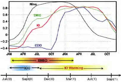
Figure 1.13. (Top) Correlation of November- January Niño3 index with SST averaged over the eastern

equatorial Pacific (160–120°W, 5°S–5°N; black), the tropical IO (40–100°E, 20°S–20°N; red), the southwest IO (50–70°E, 15–5°S; green), and the eastern equatorial IO (90–110°E, 10°S–equator; blue). (Bottom) Seasonality of the major interannual IO climate modes, IOD and ENSO. [Taken from Schott et al., 2009]

These ENSO-induced changes in deep atmospheric convection in the central Pacific have worldwide climatic impacts through atmospheric teleconnections [e.g. Trenberth et al., 1998]. Within the tropics, most of the ENSO remote impacts occur through shifts of the Walker circulation. For example, the eastward shift of the Walker circulation during an El Niño induces anomalous subsidence, increased surface solar heat flux and reduced surface wind over the IO. As a result, the entire IO basin warms during an El Niño [Figure 1.13; Klein et al., 1999; Ohba and Ueda, 2005; Xie et al., 2009]. This warming peaks in winter and spring, and can last until early summer, two seasons after the peak of ENSO, possibly maintained by local air–sea interactions over the IO [Xie et al., 2009; Du et al., 2009]. The effect of ENSO on the Indian summer monsoon has also been noted [e.g. Walker, 1924; Gershunov et al., 2001; Fasullo, 2004; Xavier et al., 2007].

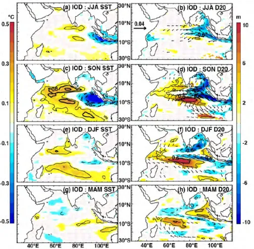
Figure 1.14. Partial regression coefficients of de-seasoned anomalies of SST (left panels), D20 (colour; right panels) and wind stress (arrows; right panels) as regressed onto the IOD index, with the

influence of ENSO removed. Regression coefficients are computed for the 1961- 2001 period and are shown when beyond a 90% significance level. Thin, normal and thick contours indicate correlation coefficients of 0.4, 0.6 and 0.8 respectively. [Taken from Currie et al., 2013]

The IOD is an independent mode of interannual variability that often co-occurs with ENSO. A positive IOD event is associated with cold SST anomalies off the coasts of Java and warm SST anomalies in the western IO, accompanied by anomalous easterlies in the central IO [Figure 1.14; e.g. Saji et al., 1999; Webster et al., 1999; Murtugudde et al., 2000]. These wind and SST anomalies grow together in a positive feedback loop [Reverdin et al., 1986; Webster et al., 1999] similar to the Bjerknes feedback involved in ENSO development [Bjerknes, 1969]. Like ENSO, the IOD is phase-locked to the seasonal cycle. It develops during boreal summer, culminates in fall, and decays by the end of the year (Figure 1.14). The IOD is usually described by the Dipole Mode Index (DMI), i.e. the difference in SST anomalies between western tropical IO (50-70°E, 10°S-10°N) and southeastern tropical IO (90-100°E, 10°S-0°N). The wind signals associated with the IOD modulate the thermocline depth in most of

the tropical IO: the anomalous easterly winds raise the thermocline in the eastern part of the basin (Figure 1.14) and, together with off-equatorial Rossby wave responses, deepen the thermocline and warm the SST in the western IO, resulting in characteristic zonal anomaly patterns in sea level height, as well as surface and subsurface temperature structures (Figure 1.14) [e.g. Feng and Meyers, 2003; Murtugudde et al., 2004; Rao et al., 2002]. Thermocline anomalies typically initiate earlier and persist longer than the surface temperature signals [Horii et al., 2008]. Negative IOD events feature opposite anomalies over similar regions [Meyers et al., 2007; Vinayachandran et al., 2002a].

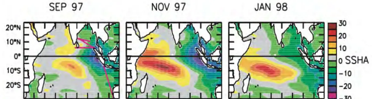
Figure 1.15. Evolution of Topex/Poseidon sea surface height anomalies (cm) during September 1997

(first column), November 1997 (middle column) and January 1998 (right column) [Taken from Rao et al., 2002]

These two interannual modes of variability (ENSO and IOD) not only influence the Equatorial IO but also strongly affect the hydrography of the BoB. Shankar [1998] first reported large negative sea level anomalies (SLAs) off the Indian east coast during 1961, one of the strongest positive IOD events on record. Rao et al. [2002] further demonstrated that the positive IOD in fall 1997 induced a negative SLA along the eastern rim of the Bay associated with an anomalous anticyclonic circulation in the BoB (Figure 1.15). Negative (resp. positive) SLAs have also been reported off the east coast during El Niño (resp. La Niña) events [Han and Webster, 2002; Srinivas et al., 2005; Singh, 2002]. However, due to the co-occurrence of ENSO with IOD events, these studies did not clearly distinguish the respective impact of these two modes on SLA in the BoB. The study of Aparna et al. [2012] addressed this issue and showed that these two modes have distinct SLA signatures, with IODs associated with a single SLA peak in fall along the rim of the Bay while ENSO exhibits weaker but multiple SLA peaks (April–December and November–July), with a relaxation between the two peaks. The northern IO response to IOD largely dominates the one to ENSO in terms of SLA [Currie et al., 2013] and mixed layer depth [Keerthi et al., 2013].

1.2.3.2. Interannual variability of freshwater fluxes

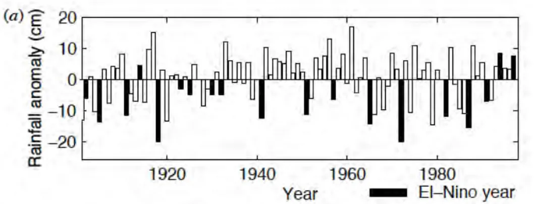
The patterns of precipitation over the BoB and adjoining continents [e.g. Gadgil, 2003] as well as the riverine freshwater supply to the BoB [Papa et al., 2012] vary significantly from year to year. The standard deviation of interannual variability of the summer monsoon rainfall amounts to approximately 10% of the long-term mean summer rainfall [Gadgil, 2003]. Precipitation in two regions, the “Western Ghats” and “Ganges-Mahanadi Basin”, accounts between 80-90% of the interannual variability of Indian continental summer rainfall [Vecchi and Harrison, 2004]. The year-to-year variability of the summer monsoon rainfall (Figure 1.16) is sufficient to trigger drought and flood conditions, with major agricultural, economic and social impacts [e.g. Gadgil and Kumar, 2006]. Many factors influence the variations of the summer monsoon precipitation on interannual timescales, including ENSO [e.g. Pant and Parthasarathy, 1981; Rasmusson and Carpenter, 1982; Meehl, 1987; Webster and Yang, 1992], the IOD [e.g. Cherchi and Navarra, 2012] and the snow cover on the Tibetan plateau and in Eurasia [e.g. Blanford, 1884; Hahn and Shukla, 1976; Meehl, 1994; Shuen et al., 1998; Wu and Kirtman, 2003]. Of these factors, the strongest association has been found with ENSO, although the relationship appears to have weakened in recent decades [Kumar et al., 1999].

Figure 1.16. Interannual variation of the all-India summer monsoon rainfall during 1901–1998; the El

Nino years are shaded. [Taken from Gadgil, 2003]

As we said already, the continental river discharges accounts for about half of the total freshwater received by the BoB [Sengupta et al., 2006]. Even though the spatiotemporal distribution of precipitation over the BoB is well documented [Xie and Arkin, 1997; Adler et al., 2003; Hoyos and Webster, 2007; Rahman et al., 2009], much less was known about the contribution of continental runoff. Recently, combining the

in-situ discharge datasets and the high-resolution satellite altimetry over rivers, Papa et al. [2010, 2012] produced interannual time series of total discharge of major rivers in the BoB over the 1993-2012 period. This river discharge dataset displays strong interannual variations of the Ganga-Brahmaputra river runoff (Figure 1.17), with a standard deviation of 12500m3/s [Papa et al., 2010].

Figure 1.17. Deseasonalized anomalies (obtained by subtracting the 16 year mean monthly value from

individual months) of the Ganga_{‐ Brahmaputra monthly river discharge at the river mouth for 1993–} 2008. [Taken from Papa et al., 2010]

1.3. The BoB salinity

1.3.1. Salinity observations

Over the recent years, the salinity observing network in the BoB has tremendously improved due to the advent of the Array for Real-Time Geostrophic Oceanography (Argo) [Roemmich et al., 2009] program and the launch of satellite missions dedicated to the monitoring of SSS salinity. As this thesis makes an extensive use of these data, the salient features of the salinity observing network in the BoB is summarized below but will be described in more details in the next chapter.

1.3.1.1. In-situ SSS observations and related climatologies

Figure 1.18. Evolution of yearly number of individual Argo profiles (ftp.ifremer.fr/ifremer/argo) from

Historically, the BoB is a poorly sampled basin (except maybe during the first Indian Ocean International Expedition). From 2002 onwards, with the advent of Argo, the number of individual profiling floats has tremendously increased (Figure 1.18), improving the observational spatial coverage compared to the historical period. The in-situ observation dataset used in this thesis (Figure 1.19a) comprises all the available in-situ SSS measurements available over the BoB during the 2006-2014 periods and will be more extensively described in chapter 2. Its coverage remains however sparse along the coast and in the Andaman Sea (Figure 1.19). This is mainly because Argo profilers with a parking depth of 1000 m, cannot access the continent shelf, which is typically shallower than 200 m. Most of the data very close to the Indian coast consist of oceanographic cruises data.

!

Figure 1.19. (a) Map of available SSS observations in the WOD09 [Boyer et al., 2009] from Argo

profilers (pink), RAMA moorings (red squares), and other datasets (green). The blue and red contours indicate ocean depths of 200 and 1000 m, respectively. The black contour delineates the area for which statistics are computed from (b) the number of observations in the western BoB as a function of the distance to the coast (in 10-km bins). Argo data are shown in pink and other datasets are shown in green. [Taken from Chaitanya et al., 2014a]

The most accurate SSS climatology in the BoB is certainly the recent North Indian Ocean Atlas climatology (NIOA) [Chatterjee et al., 2012], which is an improved version of World Ocean Atlas 2009 (WOA09) Climatology [Locarnini et al., 2010; Antonov et al., 2010]. This recent climatology includes all the data from the World Ocean Database 2009 (WOD09), complemented with Conductivity-Temperature-Depth (CTD) stations from Indian oceanographic cruises. An objective analysis gridding procedure (similar to that of WOA09), allows to fill the spatial data gaps and to smooth out the space scales shorter than 4°. The inclusion of the Indian oceanographic cruises database in NIOA considerably improves the data coverage in the periphery of the BoB compared with WOA09, especially along its western boundary [Chatterjee et al., 2012].

1.3.1.2. Remote sensing initiatives

These in-situ measurements of salinity have recently been complemented by the development of remote-sensing capabilities of ocean surface salinity (Figure 1.20). The Soil Moisture and Ocean Salinity (SMOS) European mission [Mecklenburg et al., 2008] launched in November 2009 and the Argentina/US Aquarius mission [Lagerloef et al., 2008] operating since June 2011 both provide global SSS estimates. These satellites measure microwave radiations emitted from the earth surface, at wavelengths where surface emissivity is most sensitive to ocean surface salinity. If corrected accurately from the other effects that modulate this emissivity (sea surface temperature, atmospheric composition, sea state, etc.), this allows estimating the surface ocean salinity. These new spaceborne SSS measurements are routinely validated, with global root-mean-square errors around 0.3-0.4 pss for monthly Aquarius SSS fields on a ∼150 km global grid [Lagerloef et al., 2013] and for 10-days SMOS averages on a ∼100 km grid in the tropical regions [Boutin et al., 2012]. Recent research has demonstrated the value of these satellite missions in capturing open-ocean signals related to large-scale climate modes such as La Niña signature in the tropical Pacific [Hasson et al., 2014], the IOD signature in the eastern part of this basin [Durand et al., 2013] or planetary waves signature in the southern IO [Menezes et al., 2014]. SMOS and Aquarius surface salinity products are still very new, and have not yet been thoroughly evaluated in many regions of the world. It therefore remains

unclear as to whether these satellite data can accurately capture SSS variations in relatively small basins surrounded by continental masses. The BoB, a semi-enclosed basin with a typical width of ~1000-2000 km, is indeed very challenging for satellite retrieval algorithms as the potential contamination of the SSS signal near land, such as radio frequency interference (RFI) linked to artificial sources (e.g. radars that emit in the frequency band of the instruments) and “land-induced” contamination on antenna side lobes [Reul et al., 2012; Subrahmanyam et al., 2013], could obscure climatically relevant signals there. The satellite remote sensing provides a unique opportunity to improve the monitoring of SSS variations. Hence, the arrival of these missions was a top ranking motivation for my PhD. One key advantage is their ability to sample regions that are devoid of observations.

1.3.2. Seasonal SSS variations and related mechanism

Previous studies have investigated the seasonal variations of SSS in the BoB using both observations and models [Rao and Sivakumar, 2003; Shetye et al., 1991a, 1991b, 1993, 1996; Han et al., 2001; Vinayachandran et al., 2002b; Sengupta et al., 2006; Vinayachandran and Kurian, 2007; Benshila et al., 2014; Chaitanya et al., 2014a, 2014b]. Many of the above mentioned observational studies were based on hydrographic measurements along specific shipping lanes and dedicated cruises, or historical climatologies from before the Argo era, limiting the spatial and temporal coverage of salinity profiles available in BoB.

Figure 1.21. Climatological SSS from NIOA [Chatterjee et al., 2012] for (a) summer (MJJ), (b) autumn (ASO), (c) winter (NDJ), (d) spring (FMA).

The seasonal cycle of BoB salinity estimated by the NIOA climatology is displayed on Figure 1.21. The observed SSS field displays a contrasted pattern, with fresh waters in the northeastern BoB, and saltier waters in the central and southern basin. This large-scale gradient exists all year, but is seasonally modulated. During the pre-summer monsoon season (May–June–July), surface waters with salinity below 31 are restricted to the far northeastern BoB (Figure 1.21 a). During summer monsoon, the huge river runoff and excess precipitation lead to low-salinity water in the vicinity

of river mouths in the northern BoB [Rao and Sivakumar, 2003]. As discussed in Section 1.2.2.1(c), the freshwater supply varies strongly at seasonal timescale, with about 70% of the annual inflow (from precipitation and runoff) occurring during the summer monsoon north of 15°N. The observed freshening of the northern BoB in late summer clearly follows the seasonal maximum of precipitation in June and of river discharge in August. The role of freshwater forcing in the seasonal evolution of surface salinity has already been highlighted by several studies [e.g. Shetye et al., 1996; Han et al., 2001; Sengupta et al., 2006]. With the progression of summer monsoon, the surface waters freshen the northern part of the BoB, and the freshening expands southward (Figure 1.21b). This southward expansion is especially noticeable along the eastern and western boundaries of the BoB, with clear signatures along the East coast of India at 16N and in the southeastern BoB [Rao and Sivakumar, 2003; Vinayachandran et al., 2005; Sengupta et al., 2006; Benshila et al., 2014]. The southward flowing western boundary current (EICC) play a key role in the southward export of the fresh waters during this season [Benshila et al., 2014; Chaitanya et al., 2014a]. These fresh waters start retreating back northwards in the winter, to reach their minimal extent in the spring.

Several modelling studies provided some understanding of the impacts of the freshwater forcing on the upper BoB [Howden and Murtuggude, 2001; Han and McCreary, 2001; Han et al., 2001; Yu and McCreary, 2004]. They concluded that river runoff is the dominant factor in freshening the northern part of the bay during the southwest monsoon and that lateral advection is largely responsible for the spreading of this fresh water along the east coast of India and into the AS. Most previous numerical modeling studies discussing the mechanisms of BoB SSS variability however used a relaxation toward the observed surface salinity climatology. While this strategy allows keeping the surface salinity realistic [e.g. Diansky et al., 2006; Wu et al., 2007; Sharma et al., 2010; Nyadjro et al., 2011], the relaxation term act to artificially compensate any error in the forcing or in the model physics. The relaxation term is sometimes strong in some locations of the BoB, so that it may be hazardous to infer robust conclusions about the mechanisms of SSS variability [de Boyer Montegut et al., 2005]. The aforementioned modelling studies were also suffering from a lack of realistic fresh water flux, and scarcity of validation data set.