HAL Id: hal-02191839
https://hal.archives-ouvertes.fr/hal-02191839
Submitted on 23 Jul 2019
HAL is a multi-disciplinary open access
archive for the deposit and dissemination of
sci-entific research documents, whether they are
pub-lished or not. The documents may come from
teaching and research institutions in France or
abroad, or from public or private research centers.
L’archive ouverte pluridisciplinaire HAL, est
destinée au dépôt et à la diffusion de documents
scientifiques de niveau recherche, publiés ou non,
émanant des établissements d’enseignement et de
recherche français ou étrangers, des laboratoires
publics ou privés.
The TIMMO-2-USE project: Time modeling and
analysis to use
M-A Peraldi-Frati, D Karlsson, A Hamann, S. Kuntz, J Nordlander
To cite this version:
M-A Peraldi-Frati, D Karlsson, A Hamann, S. Kuntz, J Nordlander. The TIMMO-2-USE project:
Time modeling and analysis to use. Embedded Real Time Software and Systems (ERTS2012), Feb
2012, Toulouse, France. �hal-02191839�
The TIMMO-2-USE project: Time modeling and analysis to use
M-A Peraldi-Frati
1, D. Karlsson
2, A. Hamann
3, S. Kuntz
4, J. Nordlander
51
I3S, UNSA, CNRS/INRIA, B.P. 121, 06903 Sophia-Antipolis, France. 2
Volvo Technology AB, Dept 6260 M2.7, 40508 Göteborg, Sweden.
3
Robert Bosch GmbH, Robert-Bosch-Strasse 19, 71701 Schwieberdingen., Germany
4
Continental Automotive GmbH, Siemensstrasse 12, 93055 Regensburg, Germany.
5
Chalmers University of Technology, 412 96 Göteborg, Sweden.
Abstract: The paper presents the actual results of the TIMMO-2-USE project dedicated to time modeling and analysis in the domain of automotive embedded system design. A first result is the Timing Augmented Description Language (TADL2) that offers capabilities for symbolic time expressions modeling, probabilistic timing information and timing constraints applied on mode definitions. The syntax and semantic of such extensions are presented. These extensions are aligned with EAST-ADL and AUTOSAR timing models. Based on these extensions, new algorithms and tools are developed to analyze and validate TADL2 specifications. Conjointly with these aspects, a new methodology based on industrial use cases is proposed compatible with those of TIMMO, ATESST2 and AUTOSAR. This methodology solves specific issues related to timing in an automotive system design, such as time budgeting. The TIMMO-2-USE work and results are driven by industrial use cases. Use cases are the corner stone of the project as they are used as input for providing requirements for the language, the algorithm development, and the methodology development but also because the same are used for a validation of the results.
Keywords: Time modeling, EAST-ADL, AUTOSAR, Automotive embedded systems, Use Cases, Methodology, Multi-clock systems, Probabilistic timing information,
1 Introduction
TIMMO-2-USE [1] is an abbreviation that stands for TIMing MOdel - TOols, algorithms, languages, methodology, and USE cases, which summarizes the main objectives of the project, i.e., the development of novel languages, algorithms, tools, and a methodology, validated by use cases, for the development of automotive embedded systems.
This project is the follow-up of the TIMMO project [2] which has developed a language, the Timing Augmented Description Language (TADL) [3] that allows - in the context of a development process based on EAST-ADL2 [4] and AUTOSAR 3.0 [5] - the complete management and transformation of timing information, i.e. their specification, their modeling and their analysis.
TIMMO was the path paving for introducing WCRT/WCET timing analysis into the first phases of AUTOSAR-based automotive software development. A methodology was developed – complementary to the EAST-ADL methodology - that supports these modeling
and analysis activities. Both, language and methodology were developed as true extensions of the AUTOSAR standard.
This paper presents the first results of TIMMO-2-USE. As the title suggests, TIMMO-2-USE is centered on the definition of industrial uses cases for the extension and the validation of concepts defined during the project. The definition of these industrial use cases plays a central role in the project as they drive requirements for the language, the new algorithms to be developed and methodology works.
Concerning the language, TIMMO-2-USE goes a step beyond that of TIMMO by extending TADL with new capabilities for symbolic time expressions – i.e. free variables in time expressions, multi-clock definitions, modeling of probabilistic timing information and mode dependency. Semantic definitions of such extensions are proposed that fix some previous semantical issues of TADL.
New algorithms are under development and would be integrated in some partners’ tools to analyze and validate TADL2 models.
The integration of these new results into an automotive development process is handled by the development of a methodology, compatible with those of TIMMO, ATESST2 [6] and AUTOSAR. The methodology is applied on the different industrial use cases of the project. All these aspects are illustrated on a Brake by Wire (BbW) example. This example covers one out of the four uses cases presented in this paper. The BbW system is characterized by timing requirements related to symbolic time expression, synchronization constraints and probabilistic constraints. In the paper, the example also serves as a basis for illustrating the concepts and steps of the methodology process. The algorithm results are not highlighted here but it is part of the overall picture. The paper is organized as follows: first, we give an overview of the existing work related to time modeling and methodology and we point out how we relate/differ from them. The industrial uses cases on which this work is founded are presented in section 3. Section 4 presents the Brake by Wire example and its connections with the different use cases. Section 5 is dedicated to the TADL2 language and semantics with a special focus on symbolic time expressions and probabilistic time modeling. The concepts of the methodology and how they apply on use cases are presented in section 6. A concluding section, which presents the ongoing and future works of the project, closes the paper.
2 Related work on Time modeling and Methodology in automotive domain
2.1 Timing Modeling.
An automotive design process is organized into multiple abstractions levels respectively phases which use different languages, models and tools to handle timing requirements and properties. EAST_ADL2, AUTOSAR 4.0 and their timing extensions [7] play a central role in this process. They allow expressing basic timing constraints such as repetition rates, end to end delays, synchronization and compositions of these constraints at different levels of abstraction. In these models, time is discrete and implicit. Measurements are constant values associated with two possible time units (ms and °crank). These languages consider Event as the main entity to refer to a specific location in the system at which the occurrences of such event can be observed (data read from a port, data written to a port, , activating, starting and terminating of a runnable entity, sending a frame over a network, … ), In order to relate timing events to one another, a concept EventChain is introduced. Based on
Events and EventChains, it is possible to abstract from
EAST-ADL and AUTOSAR structural models, functional and data dependencies, critical execution paths and to apply timing constraints on these paths.
The EAST-ADL timing package as well as the AUTOSAR Timing Extensions originate from the “Timing Augmented Description Language” TADL developed during the TIMMO project.
Some other languages such as the UML profiles MARTE [8] and SysML [9] make it possible to integrate in a design, more complex algebraic expressions for manipulating time. In MARTE models, time can be multiform (discrete, dense and logical). The Clock Constraint Specification language CCSL [10] is a declarative language annexed to MARTE that specifies constraints imposed on clocks. CCSL covers classical timing constraints such as the periodicity, the delay, the
offset and some others such as the precedence, the coincidence and the alternation of events. A CCSL
specification is the conjunction of all these constraints applied on clocks.
Discrete time is also a common concept for formal languages such as PSL [11] Property Specification
Language. PSL can be applied for the definition of
assertions, as well as for complex modeling. PSL also covers timing intervals based on semantics of discrete event simulation and includes a type of regular expression called SERE, a Sequential Extended Regular Expression to describe complex scenarios. In PSL, time advances in pre-defined units.
These models are independent from any abstraction level of a design. There are several tools that support PSL for simulation and formal verification (e.g. from Mentor Graphics, Cadence, and Synopsys). TimeSquare [12] is the software environment to deal with MARTE time
model and CCSL that allows timing analysis and simulation of CCSL specifications.
These languages have interesting concepts that can potentially solve some issues raised by TIMMO-2-USE. Therefore, different concepts of time: symbolic time expression, uncertain or probabilistic time, and the possibility to extend timing expression with these notions are carefully studied. TIMMO-2-USE will further advance TADL2 while keeping the current alignment between TADL2 and AUTOSAR Timing Extensions and adapting TADL2 in the future if changes of the AUTOSAR Timing Extension occur.
2.2 Methodology.
In order to accurately solve timing issues during the development of distributed automotive software-intensive systems, it is essential to follow a suitable methodology that proposes a step-by-step solution for the issue. In essence, such a methodology shall describe what needs to be done when by whom, and even more importantly, what are the required inputs and produced outputs for/by a specific step in the methodology. For efficiency reasons, it is very important that the timing modeling language provides adequate support for capturing the timing information stipulated by the methodology.
In the TIMMO [2] project, that introduced the first version of the TADL, a methodology was defined focusing on the timing analysis during a development process following the top-down approach: Time budgets on one level of abstraction are broken into smaller time budgets on the next lower level of abstraction, The primary concern of this methodology is to ensure that on every level of abstraction timing analyses are conducted in order to verify timing at early stages of the development. In addition, the methodology suggests a number of available tools for timing analysis and simulation purposes.
The ATESST2 [4] project based its methodology on the results of the TIMMO project and aligns and integrates it with other cross-cutting concerns like requirements, safety, and behavior. In addition, the ATESST2 methodology enables one to make use of various combinations of such cross-cutting concerns, for example, combining methods for dealing with safety and timing topics. This methodology accounts also for guidelines describing the sequence of task to be conducted when combining such cross-cutting concerns.
When AUTOSAR [5] introduced the AUTOSAR Timing Extensions in R 4.0.1 and maintained it in subsequent revision of this standard, the AUTOSAR methodology was extended to consider the aspect of timing in the development of automotive systems. By and large, the AUTOSAR Timing Extensions provide different timing views that are utilized during the development of the entire vehicle system (VFB and System Timing) and the development of the ECUs (SW-Component, Basic Software Module and ECU Timing) which are part of this system. The AUTOSAR methodology describes the
timing related work products to be created and maintained during the development process and which tasks require those work products.
All the mentioned methodology definitions lack the description of how timing information is used and processed while conducting tasks of the proposed methodology; and do not address various day-to-day collaboration scenarios that are playing a key role in the automotive industry, for example bottom-up approach. Specifically, the TIMMO-2-USE project is concerned about closing this gap and is addressing a number of prominent use cases and scenarios to address the timing related issues in those situations. Some of these use case are described in the following subsection.
3. T2U use case descriptions
As mentioned already above, the main goal of the TIMMO-2-USE project is to address and propose practical solutions for relevant industrial use cases that require special consideration of timing aspects. Three use-cases that are the center of discussions in this paper are described in this section.
3.1. Specify time budgets
Many novel and innovative vehicle functions span over several ECUs and across the responsibility of multiple suppliers. In the presence of timing constraints, such as maximum end-to-end latencies, that are tied to the correct functioning of such distributed functionalities, the OEM is responsible for integrating all involved system parts into the vehicle’s EE-architecture while making sure that all timing constraints are fulfilled. However, it is not clear for the suppliers what portion of the total end-to-end delay is available for the system parts that they implement. Therefore, the OEM has to divide the overall end-to-end latency for the involved system parts, and communicate these as so-called timing budgets to his suppliers. During the development process, the OEM and the suppliers want to keep the two-way feedback. When the suppliers have refined solutions at the proper abstraction level, the OEM can estimate if the time budgets are realistic, and may either ask the supplier to improve the solution or adjust the time budgets.
3.2. Specify synchronization constraints
A vehicle offers many different features such as braking, steering etc, to the driver. Today, these features are typically implemented using both mechanical and electronic components. The fact that the electronic system of the vehicle is integrated with different mechanical solutions implies that the vehicle’s electronic system inherently contains a certain degree of parallelism. That is, the system needs to monitor and control several simultaneous sources of input and output. Quite often it is also the case that the input or output needs to be synchronized in order to provide a notion of simultaneity. For example, when braking, it is crucial that the brake forces that are applied at each wheel also are applied at the same time. A correct behavior is governed by the introduction of synchronization constraints during the
vehicle design. This use-case is concerned, on the one hand, with the formulation of such synchronization constraints, and on the other hand with techniques to ensure their fulfillment during system design.
3.3 Specify probabilistic timing constraints
Much automotive functionality are so called hard-real
time systems, which means that the violation of timing
constraints leads to total system failure. For these kinds of applications it is necessary to define deterministic timing constraints such as worst-case execution times (WCET) and strict end-to-end deadlines. However, in automotive system design, one also has to cope with functionalities which can be classified as firm real-time systems. For such functionalities infrequent deadline missed are tolerable but degrade the system’s quality of service. Timing constraints for such kind of functionalities cannot be very well described using deterministic timing constraints. For this reason, this use case is about extending the TIMMO-2-USE language, methodology, and tool landscape with the possibility to specify and verify probabilistic timing constraints. In particular, it shall be possible to describe probabilistic timing properties for events and event chains. For example, the end-to-end delay of an event chain must be smaller than 10 ms in 99% of the cases. Obviously, existing methods and tools for analyzing timing constraints must be adapted. For example, the schedulability test cannot only return true or false. The answer should be the probability of the schedulability.
4. An Automotive example BbW
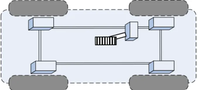
The example used to illustrate our concepts throughout this paper is a brake-by-wire system (BbW). As depicted in Figure 1, the system consists of one brake pedal, four brake actuators, four wheel speed sensors and five electronic control units (ECU).
Figure 1: Distributed architecture for brake-by-wire
Four of the ECUs are placed each at one wheel. The brake actuators and the wheel speed sensors are directly connected to the ECU at the respective wheel. The brake pedal is directly connected to fifth ECU. All five ECUs are interconnected via a common bus.
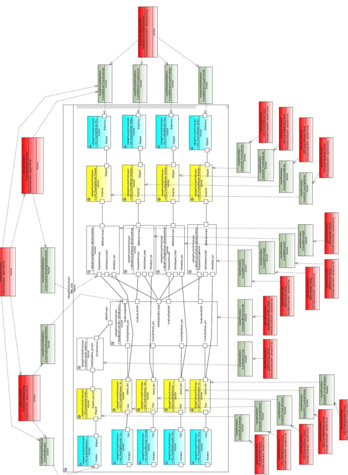
The intended functionality of this system is the following: When the driver presses the pedal, the brake actuators shall apply a braking force on the wheel that is in relation with the angle of the pedal. In addition to this basic brake functionality, it is augmented with ABS functionality in the sense that if the speed of one wheel is significantly smaller than the estimated vehicle speed, the brake force is reduced on that wheel until it regains speed that is comparable with the estimated vehicle speed. This functionality is modeled at design level in functional design architecture (FDA) as depicted in Figure 2
The FDA in Figure 2 can visually be divided into three parts. Sensors are depicted on the left, computation activities in the middle, and actuators on the right. The sensor functionality is realized with two functions for each sensor. The first function models the raw functionality of the sensors, whereas the second interprets the raw data provided by the first in the context of the application. For the brake pedal, the raw data is a certain voltage that is related to the pedal angle, which in the second step is transformed into a desired percentage of the maximal brake force. In the case of wheel speed, the raw data is “ticks”, which are interpreted as wheel speed in the second step.
The computation is divided into three main subparts. In the first subpart, the requested brake force is computed. The second subpart (solely consisting of the global controller) calculates a basic brake force on each of the four wheels, disregarding the ABS functionality. It additionally estimates the vehicle speed based on the wheel speeds. The ABS functionality is added in the second part on a per wheel basis. The desired global brake force, computed in the first step, may be adjusted depending on the difference between the estimated vehicle speed and the respective wheel speed.
The actuator part has a similar two-steps structure as the sensors, but mirrored. The first step translates the requested brake force into an electrical voltage that can be used by the actuators in the second step.
All wheel-specific functions are allocated to the ECU near their respective wheel. Functionality related to the pedal and to the global controller is allocated to the central ECU.
This design is primarily concerned with two types of timing requirements: end-to-end latency and synchronization. The end-to-end latency requirements constrain the time it might take for the brake actuators to react to a change of the pedal angle. As shown in Figure 2, this limit is in this example set to 200ms. The figure also shows two segments of this delay of 130ms and 70ms. Although not explicit in the figure, identical requirements are imposed for all wheels.
The end-to-end latencies introduced previously only state an upper bound on the response from pedal angle change to a brake actuation. For that reason, a situation where the front left wheel starts braking after 50ms and the front right wheel after 200ms would be legal. Such behaviour could potentially be dangerous, or at least very
uncomfortable to the driver. In order to enforce the brake actuation to happen roughly at the same time at all wheels; regardless of if it happens after 50 or 200ms, a synchronisation constraint is introduced. The synchronisation constraint states that if one actuation event occurs on one wheel, actuation events must also occur on the other wheels within 20ms.
In addition, each function has been assigned a period. All functions in the sensor and actuator parts have a period of 10ms, whereas all functions in the computation part have a period of 50ms.
5. The TADL2 language
TADL2 is a language for imposing timing constraints on the events identifiable in structural models on different levels of abstraction. As such, TADL2 is entirely agnostic regarding the nature of the events it constrains, demanding only that it must be possible to associate every event with a sequence of occurrence times when a modeled system is run. Currently, TADL2 incorporates the event definitions of both AUTOSAR and EAST-ADL, as well as a more informally identified form of external events.
5.1 Overview of the language
The timing constraints of TADL2 are of three basic forms:
• The repetition constraint, which constrains the distance between repeated occurrences of a single event.
• The delay constraint, which constrains the distance between two events called source and
target, so that all occurrences of source must be
matched by an occurrence of target.
• The synchronization constraint, which
constrains a set of events to always occur within a certain tolerance from each other.
From these basic constraints TADL2 derives several forms that capture common special cases and offer compatibility with AUTOSAR 4.0 timing extensions. Typical examples are the special cases of periodic and
sporadic repetition, and the delay variants age and reaction time (which attach to the event-chains used to
indicate causality relationships between events in AUTOSAR).
The BbW system modeled in Figure 2 illustrates the use of all three basic constraints. The delay constraint
BrakeReactionDelay at the top of the figure specifies that
the upper limit on the distance between each occurrence of EventPedalPosition and the matching occurrence of
EventABSTorqueRearRight is 200 milliseconds. The
lower limit, which is also possible to specify, defaults to 0 if not present.
The bottom of Figure 2 also shows fifteen examples of periodic repetition constraints, with periods varying between 10 and 50 milliseconds. Each such constraint is equivalent to a basic repetition constraint giving equal values for their upper and lower distance limits. It is important to note that these constraints—just like the delay constraints above—are just specifying requirements on the functions producing the constrained events; they are in no way part of the implementations of these functions.
The rightmost constraint of Figure 2 illustrates the third basic constraint form: event synchronization. In this case four individual events are constrained to always occur within 20 milliseconds of each other, although without prescribing any form of order between them (this is the essential difference between synchronization and a set of delay constraints). Whether such a timing behavior is allowed, contradicted, or maybe even implied, by the other constraints attached to the same events is a separate question that can only be answered by comparing the meanings of all constraints involved.
To simplify reasoning, TADL2 defines the semantics of each of its basic constraints formally, using only logical quantifiers (for all, there exists) and simple inequalities between time values. The meaning of derived constraint then follows from their mechanical translation into the basic forms.
5.2 Symbolic time expressions
All time values in Figure 2 are simple constants, which is often all that is needed in order to specify a desired timing behavior. However, one of the main developments of TADL2 is the generalization of time values to expressions that also include symbolic variables and arithmetic operations. The three delay constraints of Figure 2 may illustrate the power of this extension. Since a given delay limit must be preserved when an end-to-end delay is broken down into segments, the presence of two segments in Figure 3 actually only corresponds to one degree of freedom when setting up a time budget for the segments. Thus, instead of manually maintaining the invariant that the upper limits assigned to BrakeDelayAtMasterNode and BrakeDelayAtRearRightNode always sum up to 200 ms, it may be beneficial to express this invariant by giving the upper attribute of BrakeDelayAtRearRightNode the value of 200 ms - BrakeDelayAtMasterNode.upper. Furthermore, by replacing 130 ms in BrakeAtMasterNode by the symbolic expression x ms, it will be possible to freely experiment with different values of x, as well as to symbolically infer possible bounds on x as dictated by other constraints (in this example, x must clearly be between 0 and 200 for the constraints to be satisfiable at all).
5.3 Multiple timebases
Timing constraints traditionally refer to the universal chronometric time which is implicit in constraint declaration. This convenience presents two main drawbacks. First, it is difficult to model constraints measured on a different timebase so as for an ignition
control system where timing constraints are both measured on chronometric clocks or/and rotation angle of a crankshaft. In this case, the rotation position of the crankshaft triggers periodic execution of control functions. Secondly, as clocks are implicit, drifts, jitters and offset between clocks cannot be modelled easily. This is a classical issue when distributing functions code on different ECUs. The choice of a processor and/or a network may introduce distortions on time evolution that influences the overall constraints.
To overcome these drawbacks, we propose, in TADL2, an explicit notion of timebases. A timebase represents a possibly infinite and strictly ordered set of instants. A timebase is associated with a dimension. Example 1 shows how to declare a dimension. A time measurement may have a chronometric or an angle dimension. Each dimension lists their units. Numbers indicate the ratio between one unit and the smallest one (ratio=1). Thus, the timebase Universal is of type chronometric and its precision is the nanosecond (ns).
dimension chronometric { ns:1, micros:103, ms: 106,
sec: 109}
dimension angle { degree: 1, rotation: 360 } timebase Universal: chronometric { 1 micros } timebase ECU1: chronometric {1 ms on ECU1= 96
micros on Universal }
timebase Crankshaft: angle {1 rotation on Crankshaft
= speed ms on Universal }
Example 1: Dimension and timebase declarations
Timebases may relate to each other. As shown in example 1, ECU1 has a drift of 4 micros comparing to the
Universal timebase.
Timebases with different dimensions can be linked as well. For instance, the cranckshaft timebase has an angle dimension. A conversion factor based on the engine rotation speed must be applied on values measured on the crankshaft to be converted into the Universal timebase. Arithmetic rules have been defined to cope with multiple timebases and timingExpression with values measured on multiple timebase. Based on this definition of Universal, a timing expression in the BbW example becomes:
DelayConstraint.Lower = 200 ms on Universal
5.4 Probabilistic time
A basic delay constraint defines time windows in which target occurrences are expected, but does not further specify where in such a window an occurrence should be placed. This means that a behavior where the target occurrences repeatedly touch the window limits is just as correct as a behavior where occurrences are nicely concentrated to the window midpoint. To give the constraint user a means to distinguish between such behaviors, TADL2 has been extended to support the
notion of probabilistic timing. Two complementary approaches are currently included in TADL2 side by side. One approach assumes full independency between repeated occurrence variations, which allows occurrence placements to be finely controlled using an optional
distribution attribute. Available settings include both
predefined standard distributions as well as arbitrary discretized distribution curves. The other approach needs no independence assumption but requires the parallel use of several constraints to express variations, each one specified with an attribute that expresses a minimum number of inhabited time windows over sequences of a particular length.
The two approaches are overlapping, but their detailed relationship is still a topic of further investigation within the TIMMO-2-USE project. Ongoing work is also exploring how the probabilistic approaches can be applied to the other basic constraint forms of TADL2.
5.5 Timing constraints and modes
Even TADL, the constraint language of the original TIMMO project, supported a notion of system-level mode identifiers attached to its timing constraints. TADL2 inherits this mechanism, with the intuition that a mode-dependent constraint only needs to be satisfied during the intervals when its mode is active. The mode concept is a quite complex idea, however, whose full specification and realization involves much more behavioral aspects than just a desired timing behavior. Still, the logic of mode changes does affect the meaning of timing constraints, since changes that occur during some open time window may render the window inhabitance question ambiguous. To keep the TADL2 language relatively self-contained, TIMMO-2-USE has decided not to fully develop the logic of modes and mode changes, but to capture their impact on timing constraints via a notion of start and stop events for each mode. This means that ambiguity issues related to the timing of mode changes can be sorted out semantically in TADL2 without having to engage in all aspects of defining and propagating mode changes throughout a full system model. The exact definitions of mode-dependent repetition, delay and synchronization constraints is still work in progress.
5.6 Gap between AUTOSAR and EAST_ADL concepts
TADL concepts of events, event chains, and timing constraints are common to AUTOSAR Timing Extensions introduced in AUTOSAR R4.0 and EAST_ADL. In TADL2, timing constraints have been revisited by clarifying semantic points such as the timing constraint in the context of mode or the synchronization constraint. New concepts have been introduced such as the symbolic timing expression and the explicit clock definition. The objective of TIMMO-2-USE is the ownership by AUTOSAR and EAST_ADL of these new concepts by aligning them to the current and future releases of these languages.
6. Methodology 6.1 TIMMO-2-USE Generic Method Pattern
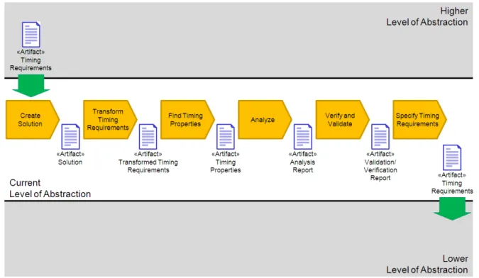
During the analysis of several industrial use cases it became obvious that there are a lot of common tasks. This led to the definition of the TIMMO-2-USE Generic Method Pattern (GMP) described in this section. This method pattern is the basis for all steps to be taken during the course of a phase and level of abstraction respectively. As shown in Figure 3, the TIMMO-2-USE Generic Method Pattern consists of the six tasks called “Create Solution”, “Transform Timing Requirements”, “Find Timing Properties”, “Analyze”, “Verify and Validate”, and “Specify Timing Requirements”. By and large, these tasks are carried out at every level of abstraction of the EAST-ADL. Since the EAST-ADL, as well as TIMMO-2-USE, defines a phase for every level of abstraction these tasks are carried out for every level of abstraction: Vehicle, Analysis, Design, Implementation and Operational Level. Indeed, there are two exceptions: The first exception is that at the beginning of the Vehicle Phase, a formal work product “Timing Requirements” is not available. The second exception is that at the end of the Operational Phase the task “Specify Timing Requirements” is not carried out. In the following, all tasks and their purpose are described in more detail. The tasks are described in the order as they appear in Figure 3 (from left to right).
Create Solution: Based on the given requirements, including timing requirements, that originate from the higher level of abstraction respectively previous phase, a solution is created or an already existing solution is revised. While creating/revising the solution the given timing requirements must be considered, in other words the given timing requirements, like any other non-timing requirement, guide the creation of the solution. The resulting solution is captured in appropriate models. In case of EAST-ADL these models are the Technical Feature Model TFM on the Vehicle Level, Functional Analysis Architecture FAA on the Analysis Level, Functional Design Architecture FDA and Hardware Design Architecture HDA on the Design Level, and Environment Model EM which is present on all levels of abstraction. Out of these, the first three models primarily capture timing requirements and properties related to the system’s application. The Hardware Design Architecture provides parameters for execution and hardware delays. The Environment Model provides characteristics and constraints imposed by the surrounding systems.
Several solutions (alternatives) can evolve from the task “Create Solution” and each of those solutions shall have the potential to satisfy the given requirements. However, each solution may result from specific design decisions that have been taken during the course of this task.
Transform Timing Requirements: Based on the created solution the timing requirements specified in the previous phase are transformed into timing requirements suitable for further processing during the current phase. In other words, those timing requirements are transformed into timing requirements such that they are “comparable” with the timing properties of the solution created in the current
phase and thus on the current level of abstraction (see also the description of the task “Verify and Validate”).
In a nutshell: Timing requirements are expressed using events, event chains, and timing constraints that are imposed on these events and event chains. Events refer to locations, usually ports, in a solution model at which the occurrences of the events are observed; and event chains specify a causal relationship between events and their temporal occurrences.
During every phase, a solution model is created based on the requirements and solution model created in the previous phase. An event specified in the previous phase
and referring to an observable location in the corresponding solution model possibly has to be transformed or mapped into an event referring to an observable location in the solution model created during the current phase. This transformation has to be performed for all events and event chains, and especially the values of the timing requirements imposed on event chains.
Several solutions (alternatives) can evolve from the task “Create Solution” and for each of those solutions the given timing requirements must be transformed.
Figure 3: TIMMO-2-USE Generic Method Pattern.
Find Timing Properties:. Once the solution has been created and the timing requirements evolved from previous phase have been transformed [into timing requirements on the current level of abstraction], the timing properties of this solution are specified and the values of these timing properties are determined and assessed. The methods applied to determine – find – the particular values are manifold: [timing] expert knowledge and estimation, simulation, analysis, educated guess, knowledge from previous projects or iterations within the current project, etc. The most appropriate and suitable method should be selected for this purpose.
The objective of this task is to find timing properties that are inherent in the solution and its requirements. For example, the critical path in the solution is identified and annotated with timing properties accordingly.
Note that the purpose of this task is not to define new types of timing properties, but to decide which of the timing properties, like latency, response time, execution time, sampling rates, etc. are used to describe the dynamic behavior of the solution.
If several solutions (alternatives) are available, then each of those solutions is annotated with timing information. And with regard to the dynamic – temporal – behavior of the solutions there may be different critical paths leading to different sets of timing properties and their values.
Analyze: Based on the solution and its timing properties the specific values of those timing properties are assessed, in the sense of checking the consistency of all timing properties (looking at the whole picture and the target system). The primary purpose of this assessment is to decide whether to continue conducting the subsequent tasks in the development process, or to repeat any or a sequence of previous tasks. In other words at this point it is decided “whether the numbers are good enough for progressing”, or whether those numbers have to be revised (iteration). It could also happen that the solution subject to timing analysis must be revised, or even worse a new solution must be searched.
The methods applied to assess the values of the timing properties are manifold and the most appropriate and suitable method should be selected for this purpose. Such
a method could be as simple as an addition of values, or it could be more complex, like applying a calculus on the given numbers. In addition, the methods being used for analyses may vary depending on the phase: On higher levels of abstractions other methods are used than on lower levels of abstraction. For example, scheduling analysis is used on implementation level, but not on abstraction levels like Vehicle Level.
It may happen that several solutions (alternatives) are available and in this case the purpose of the task “Analyze” is to identify and quantify the strengths of every solution with regard to the dynamic – temporal – behavior. One can select the most appropriate and/or promising solutions in order to proceed with the development.
Verify and Validate: Eventually, the timing properties are explicitly compared against the given timing requirements (verification) and assessed for appropriateness, which means regarding consistency and correctness (validation). During the course of this task the values of the timing properties are compared against the values of the
transformed timing requirements and possibly timing
properties that arose during the course of the phase. The primary purpose of this task is to decide whether to continue conducting the subsequent tasks in the development process, or to repeat any or a sequence of previous tasks. Essentially, this is the task which “compares the numbers of timing properties with given [transformed] timing requirements”.
If several solutions (alternatives) are available then the purpose of the task “Verify and Validate” is to verify and validate the timing properties of every solution. One has to select the most appropriate solution – one solution – in order to proceed with the development.
Specify Timing Requirements: Once the decision is taken to proceed with the next phase, all or some of the
obtained timing properties and transformed timing requirements are converted into corresponding timing requirements.
The result of the task is not that all timing properties that were found in the previous tasks are converted into timing requirements, but only those of them which are fundamental and important for design decision to be taken in subsequent steps. One criterion for identifying timing properties as timing requirements is that they were critical for the verification performed.
These timing requirements are the basis for any design work being conducted during the next phase.
In the TIMMO-2-USE project the Generic Method Pattern is used in the work package “Methodology” to describe the various use cases identified at the beginning during the requirements elicitation in work package “Requirements and Use Cases”. The following section makes use of this pattern explaining the tasks to be carried out in order to specify time budgets on different levels of abstraction and phases respectively.
6.2 Use case Specify time budgets
In
Figure 2, an end-to-end latency between pedal sensor
and brake actuator of 200ms has been specified at higher abstraction levels and given to this abstraction level as a requirement. The task is now, in accordance to the description of the use case Specify time budgets in section 3 to divide this end-to-end latency over the intermediate design functions. For simplicity of example, we assume that it is sufficient to divide the end-to-end latency into two segments as indicated in the figure. The focus is here on the first segment, BrakeDelayAtMasterNode. Figure 4 presents the methodology for the use case Specify time budgets, and how it maps to the generic methodology presented in section 6 The Find timing properties and theAnalyze timing properties tasks have been split into two
subtasks each in order to illustrate the activities to be performed in these tasks in more detail. Moreover, the tasks Verify timing properties and Specify timing
requirements have been renamed to better reflect their
purposes in the context of this use case. The following paragraphs will describe the figure in more detail focusing on the tasks mapped to Find timing properties and Analyze timing properties: The task Find timing properties identifies timing properties with a direct impact on the time budgeting process and that are a direct implication of the solution and its timing requirements. Such properties are typically execution times (or preferably response times) and communication delays. These properties can be obtained using the following strategies:
1. Transformed from a lower abstraction level 2. Determined from the solution
3. Determined from an extrapolated solution at lower abstraction level
Each of these strategies is represented by a separate task in the methodology.
The purpose of the task Transform time budget properties
from lower abstraction levels is to reuse information that
Solution Time budget [Higher level] F in d ti m in g p ro p e rtie s A n a ly z e ti m in g p ro p e rtie s Time budget properties [Lower level] Create solution Transform time budget properties from lower AL Determine time budget properties Estimate influence from future functionality
Create time budget proposal
Verify time budget
Specify time budget
Estimated influence from future functionality Time budget proposal Time budget verification report Time budget Extrapolate time budget properties
Time budget properties Product plan
Figure 4. Methodology for the use case Specify time budgets
has already been derived for the parts of the solution that has already been developed bottom-up at a lower abstraction level. Referring to the example inFigure 2, the WCET of the HW_BrakePedalSensor and the LDM_BrakePedal have been determined/measured at a lower abstraction level, but are in this task transformed into the context of the current abstraction level with values of 5ms each.
The task Determine time budget properties analyses the solution and its requirements for time budget properties that are a direct implication of the solution and the requirements at the current abstraction level. In our example, this corresponds to highlighting all periodic constraints on all functions, including those of the sensor functions whose execution times we estimated in the previous task.
The task Extrapolate time budget properties addresses a problem that occurs in particular at high abstraction levels, where information needed for finding the sought timing properties might not be present. The task allows us to rapidly prototype lower-level models in order to estimate essential properties. In our example, this task is not necessary as all functions are annotated with periods. In the task Analyze timing properties, the previously found timing properties are elaborated to form a time budget proposal. In this process, not only the current solution needs to be considered, but also the influence of both planned and still unknown future functionality. The task Estimate influence from future functionality assesses the amount of slack that needs to be introduced due to interference of future functionality. In our example, we disregard this aspect.
A final time budget proposal is formed in the task Create
time budget proposal based on the identified time budget
properties and the estimated influence from future functionality. The principal timing properties needed for creating a time budget in our example, are the periods of function. Given the assumption that the execution times are less than or equal to the period (which we have in some cases even confirmed previously), the periods are the main contributors to the end-to-end response time. Summing up the periods gives a delay of 110ms. Assigning a budget of 130ms to this part of the system therefore introduces a 20ms margin that may be used for a more relaxed implementation if needed in the future. Following the same line of reasoning, the second budget segmented was fixed to 70ms. Both budget segments give a total latency of 200ms, which satisfies the original requirement.
Lower abstraction levels will receive the two budget segments as requirements in addition to the end-to-end latency requirement.
7 Conclusion & perspectives
This paper presents the first results of the TIMMO-2-USE project concerning the time modeling and analysis of automotive embedded systems. Different uses cases are defined in the project which highlights new needs to
consider such as complex time expression with variable parameters, multi time bases and probabilistic values. A methodology has been developed that covers these use cases. A TADL2 language guide is currently being prepared. Results on analysis and new algorithms to validate TADL2 models are not highlighted in the current paper but it is part of the all picture.
Ongoing work will further advance TADL2 while keeping the current alignment between TADL2 and EAST_ADL2 and AUTOSAR4.0 timing concepts. Collaborations between the MAENAD project and the AUTOSAR timing group will allow adapting TADL2 if future changes of the AUTOSAR and/or EAST_ADL timing concepts occur.
Acknowledgment
This document is based on the TIMMO-2-USE project in the framework of the ITEA2, EUREKA cluster N°3674. The work has been funded by The French Ministry for Industry and Finances, the German Ministry for Education and Research (BMBF) under the funding ID 01IS10034, and the Swedish governmental agency for innovation systems (VINNOVA). The responsibility for the content rests with the authors.
8. References
[1] TIMMO-2-USE Project, ITEA 2, 2009, Website
http://www.timmo-2-use.org
[2] TIMMO Project,, ITEA2 2007, Website
http://www.timmo-2-use.org/timmo/index.htm
[3] H. Blom, R. Johansson, H. Lönn. Annotation with Timing Constraints in the Context of EAST-ADL2 and AUTOSAR – the Timing Augmented Description Language. STANDRTS'09 at ECRTS 2009. Dublin, Ireland, June 2009
[4] EAST_ADL2 – ATESST Project: EAST_ADL2 Specification, profile and Tools http://www.atesst.org
[5] AUTOSAR AUTomotive Open System Architecture.
http://www.autosar.org
[6] ATESST2 Project, FP7 STREP, ICT for Transport, EUCAR Integrated Safety Program, June 2008 to June 2010. http://www.atesst.org
[7] AUTOSAR Specification of Timing Extensions, 1.1.0, AUTOSAR Release 4.0.2, 2010-11-03, AUTOSAR Development Cooperation.
[8] OMG UML Profile for Modeling and Analysis of
Real-time and Embedded Systems, MARTE V1.0.
Object November 2009. OMG document number: formal/2009-11-02.
[9] OMG. Systems Modeling Language (SysML) Specification 1.1. Object Management Group, May
2008. OMG document number: ptc/08-05-17
[10] C. André. Syntax and semantics of the clock constraint specication language. Technical Report 6925, INRIA, 2009.
[11] IEEE P1850 - Standard for PSL - Property Specification Language Homepage
http://www.vhdl.org/ieee-1850/, March 2011.
[12] TimeSquare Model Development Kit,
http://www-sop.inria.fr/aoste/dev/timesquare/