When Promotions Induce Good Managers to Be
Lazy
Frédéric Loss (CNAM) et Antoine Renucci (CEREG)
When Promotions induce Good Managers to be Lazy
∗
Frédéric Loss
†Antoine Renucci
‡Abstract
In our context, a good-reputation manager favors risk when being perceived as good allows to be promoted while risk is observable but not verifiable. Indeed, it renders more difficult the learning process regarding her talent. In turn, this lowers her level of effort since the extent to which effort impacts the perception the market has about her talent is lessened. We show how and when monitoring helps employers restore incentives to work. By contrast, career concerns discipline a bad-reputation manager in our context, provided that promotions are sufficiently attractive. These results hold when two managers of heterogeneous reputation compete for one position.
∗We are grateful to Bruno Jullien and to Denis Gromb, for their encouragements and numerous suggestions. We also want to
thank Bruno Biais, Guido Friebel, Alexander Guembel, Carole Haritchabalet, Estelle and Leatitia Malavolti, Javier Ortega, Paul O yer, P ierre P icard , J ean T irole, A n ne Van h em s and W ilfried Z antm a n.
†Conservatoire National des Arts et Métiers, Paris ‡U n ive rs it é Pa r is-D a u p h in e
I. Introduction
Career concerns “arise whenever the (internal or external) labor market uses a worker’s current output to update the beliefs about the worker’s ability and then bases future wages on these updated beliefs” [DeMarzo and Duffie, 1995]. Since promotions are based on the assessment by the market of a worker’s ability, they also create career concerns. Yet, they have so far received little if no attention in a career concerns context. This is unfortunate since the discontinuity in the revenue of the worker promotions accompany can distort the incentives the latter faces. This is also surprising since such revenue discontinuities occur in many contexts other than managerial promotions: When engineers in a R&D laboratory try to create their own firms or general partners with a venture capital fund search investors to set up another fund at better conditions. When managers of a sector fund seek to manage a larger fund or a growth or growth and income fund, or CEOs want to seat on the board of another firm.
In this paper, we investigate delegated risk-taking and its consequences on effort provision when managers face promotion opportunities. Indeed, the perspective of hitting the jackpot has the potential of influencing one’s behavior regarding risk. The following questions motivate this paper. What is the impact of the perspective of a promotion both on the risk-taking policy the manager opts for and on the effort she exerts, when her ability is uncertain? Does this impact depend on the current reputation of the manager? What is the reaction of her employer? What does change when two managers are competing for one position instead of competing against an exogenous benchmark?
To answer the first three questions in the simplest way, we start with a standard two-period career concerns model a la Holmström [1982, 1999]. Managers of uncertain quality work within companies. Uncertainty regarding each manager’s ability stands from the fact that either the manager begins her professional life or she has just switched over to a new job. Information is incomplete but symmetric at the beginning of the first period. The
market only forms initial beliefs regarding the manager’s talent, i.e. the manager has a reputation. Initial beliefs are updated with respect to available information, e.g. the manager’s output, at the end of the first period.
We depart from the standard model along several dimensions. First, by considering that the manager can be promoted at the end of the first period provided that her updated reputation is good. Promotion implies a substantial wage increase. Next, by assuming that the manager attempts to influence the market’s beliefs through a choice of risk policy and a choice of effort. Crucial to the model is the assumption that the risk of the action-the manager chooses between two projects of different risk -is observable by action-the market but not verifiable. Finally, by allowing the employer to use a public report on the manager’s activity- and not only accounting profits -in the learning process. These two sources of information differ for two reasons. First, the manager manipulates the accuracy of the information content of the profits by realizing a more or less risky action, whereas she cannot influence the accuracy of the information contained in the report. Next, and symmetrically, employers choose the accuracy of the information content of the report, e.g. hire a supervisor to monitor the manager, but cannot impact the accuracy of the information content of the profits.
We analyze how the perspective of a promotion influences the willingness of a manager to let the market learn information regarding her characteristics as well as her employer’s willingness to gather this information. In this respect, the manager’s initial reputation is essential. The latter is either “good” or “bad”, depending on whether it is above or below the threshold that allows the manager be promoted. A manager with a good reputation wants the market to keep its a priori about her talent. Therefore, she opts for the riskier action so as to limit the updating process. Indeed, a very risky action makes it difficult to infer from its outcome whether success is due to fortune or managerial talent, and whether failure occurs because of bad luck or a lack of managerial skills, since the market has observed that the manager took a lot of risks. However, choosing the riskier action induces the manager to reduce her level of effort since the extent to which effort impacts the perception the market has about her talent is lessened. This negatively affects the value of the firm she works in. By contrast, a bad-reputation
manager wants the market to change its beliefs regarding her ability. Hence, we show that, provided that the additional revenue is attractive enough, she chooses the less risky action to facilitate the updating of beliefs process: The result of the project is more informative about the manager’s ability because of the low level of risk involved.
In most cases, the employer monitors the manager which improves the accuracy of the information regarding managerial talent and induces the manager to exert a higher level of effort than she would otherwise perform. However, as monitoring is costly, it never eliminates accounting profits as a source of information. Overall, an employer monitors more intensely a manager if the latter has chosen the riskier project rather than the less risky project. Next, for a given manager, an employer exerts a higher monitoring effort when this manager has a good rather than bad reputation for a comparable distance between the manager’s assessed talent and the reputation level that allows her to obtain a promotion. In some other cases, i.e. when the manager opts for the less risky action, when this action implies a particularly low level of risk so that accounting profits are especially accurate, the employer does not to monitor the manager.
Finally, and in order to answer the forth question, we examine the situation where two managers of hetero-geneous reputation compete for one position at a higher level. Interestingly, the result that the good-reputation hence the favorite in the competition -opts for the riskier project whereas the bad-reputation manager-hence the outsider -opts for the less risky project still holds, provided that the promotion is sufficiently attractive. This result stands in contrast to the conventional wisdom that winners at an interim stage choose a safe strategy to secure their position whereas laggards have “nothing to lose”, and consequently gamble. The conventional result relies on the choice of risk not to be observable.
The present research builds on the career concerns literature which starting point is that superior performances generate high wage offers whereas poor performances generate low wage offers [Fama, 1980]. This literature devel-ops the idea that managers try to influence the perception the market has regarding their ability by manipulating
performances. Either they exert effort to inflate their output [Holmström, 1982, 1999], which is positive for the firms they work with. Or they modify the accuracy of the information that accrues to the market by herd-ing [Scharfstein and Stein, 1990], by resortherd-ing to hedgherd-ing technics [DeMarzo and Duffie, 1995, Breeden and Viswanathan, 1998], by choosing the risk of the project they realize [Holmström, 1982, 1999, Hermalin, 1993], or by avoiding to undertake projects that would deliver information regarding their talent [Holmström and Ricart I Costa, 1986]. In this respect, the existence of career concerns does not discipline managers1. One of the novelties of the present paper is to examine the interaction between risk-taking and effort-performing when managers have career concerns. Consequently, it investigates the interaction of the two opposite effects mentioned above.
Besides, to the best of our knowledge, the career concerns literature [e.g. Dewatripont, Jewitt and Tirole, 1999, part I2] has so far ignored the opportunity to improve the learning process by resorting to a source of information the accuracy of which does not directly depend on the manager’s decision. For example, in the herding stream of this literature [Scharfstein and Stein, 1990], the market takes into account two signals, i.e. the result of a project and the comparative actions of the managers, but these sources of information directly depend on the manager’s actions. By contrast, we investigate how and when monitoring, the accuracy of which only depends on the employer’s decision, helps the employer restore incentives to work.
As usual in career concern models, we explore a situation where managers and the labor market share the same information, which makes sense when managers are at the early stages of their careers or when they switch for another job requiring a different talent. However, because managers are clearly identified as having a good or a bad reputation, and because reputation plays a role in our context, the framework we develop here allows us to derive different behaviors. This is different to Zwiebel [1995], Prendergast and Stole [1996], or Breeden and Viswanathan [1998] where different behaviors are obtained because managers have private information regarding their abilities.
1See also influence activities [Milgrom, 1988].
The paper is also connected to the literature on promotions. It seems likely that promotions primarily serve the purpose of moving people to tasks where their comparative advantage is highest, i.e. matching higher level jobs with higher ability [see Sattinger, 1975, Calvo and Wellisz, 1979, Rosen, 1982]. When the current employer has information on his manager’s ability, while the external labor market can only observe job assignment, the current employer decides on who to promote strategically to avoid large wage bills as wages respond to outside options [Waldman, 1984]. If the manager also has private information, there are opportunities of screening for the employer by proposing a menu of contracts among which the employee self-selects [Ricart I Costa, 1988]. When employers have discretion regarding the speed of promotion, they use that variable to adjust the information they convey to the market [Bernhardt, 1995]. Overall, these papers assume informational asymmetries- while we do not focus on that point -and do not investigate the incentive properties of promotions. The latter were extensively studied in tournament settings. However, tournaments do not account for the heterogenous reputations we consider.
The paper is organized as follows. In Section II, we introduce the model and discuss the most important assumptions. In Section III, we assume that accounting profits are the only source of information. Then, we derive the optimal behavior of a manager regarding her choice of risk and her resulting choice of effort. In Section IV, we examine these choices when employers can resort to monitoring. We also discuss the relation of the paper with the existing literature and propose implications. In Section V, we turn to the case where two managers of heterogenous reputation compete for a promotion. Concluding remarks follow. Proofs are supplied in the Appendix.
II. The Model
employing a manager each. All parties are risk-neutral. During the first period, all managers lie at the same level in the hierarchy. We restrict our attention to the representative manager-firm pair.
II.A. First Period
The accounting profits Π1 derived from the manager’s activity are given by
Π1(θ, rp1, e1) = θ + rp1+ e1, (1)
where θ is the manager’s talent (or ability), rp1 is the risk of the project p realized by the manager in the first
period, and e1 is the manager’s first-period effort.
The manager’s exact talent θ is unknown. However, it is common knowledge on the labor market that θ is drawn from the distribution θ ∼ N(E(θ); σ2θ). Thus, information is incomplete but symmetric. Either E(θ) ≥ θ
and the manager’s reputation is “good ” or E(θ) ≤ θ and the manager’s reputation is “bad”.
The manager has to choose the project p she undertakes, with p ∈ {A, B}. Project A defined by rA∼ N(0; σ2A)
is less risky than project B defined by rB ∼ N(0; σ2B) in the sense that σ2B > σ2A. Observe that the risk of the
project has no direct impact on its expected profitability.
Essential to the model is the fact that the choice of project is observable3 by the market but not verifiable. As
Hermalin [1993] suggests, this assumption makes sense in a variety of contexts: Stock analysts evaluate projects’ risks while boards of directors should have this expertise. Even the business press sometimes publicizes the assessments of the risks of new projects. Insiders in the mutual fund industry observe the risk-profile of the portfolios that managers hold even though it is difficult to assess for the public. Employers have privileged information regarding the hedging policies their managers follow even though Generally Accepted Accounting Procedures do not impose on these managers to publicly disclose their hedging decisions. No contract can be
3Biais and Casamatta [1999] in the spirit of Jensen and Meckling [1976] also study the case of managers exerting effort and
choosing the risk of their ventures, but both choices are unobservable in their paper which differs from our assumption that the choice of risk is observable. Moreover, they examine explicit incentives whereas we consider implicit incentives. The latter remark applies for Hvide [2000] in a tournament setting. As for observability of the risk-taking policy, Hvide successively investigates the two cases. See also Diamond (1998).
contingent on the choice of risk since this choice is not verifiable.
Once the manager has decided which project to undertake, she exerts an unobservable level of effort e1. This
effort costs her ψ(e1), with ψ0> 0 and ψ00> 0.
The firm (also referred to as the employer or he) has access to a monitoring technology (e.g. hire a supervisor or an auditor) that produces a report τ1. He decides the precision of the report, once the manager has selected
the project p, but before she exerts the effort e1. Let 1 (with 1∼ N(0; σ21)) represent an observation error.
Setting up a monitoring technology that costs c¡σ2
1
¢
(with c0< 0, c00> 0, c(∞) = 0, c0(0) = −∞ and c0(∞) = 0)
allows the employer to choose σ21 as monitoring level. The market can observe the precision that each employer opted for. The report
τ1(θ, e1, 1) = θ + e1+ 1 (2)
is delivered once the manager has exerted her effort.
The profits and the report are observable by everyone so that the manager has a reliable track record to exhibit to the labor market which allows her to obtain a second-period position that depends on her first-period output. Yet, we do not analyze explicit contracts in what follows. In the tradition of Holmström [1982, 1999] or Scharfstein and Stein [1990], we assume that a manager cannot be bound to her firm against her will ex post. This implies that any long-term contract that would pay a manager less than the spot market wage in the second period is infeasible. Of course, a short-term incentive contract could serve to help align manager’s and firm’s interests, by specifying a profits-contingent wage in the first period. Thus, in principle, a manager could be induced to act so as to maximize a weighted average of the firm’s expected profits and her future compensation. However, this more general formulation leads to the same qualitative results (see Scharfstein and Stein [1990], Prendergast and Stole [1996], as well as Breeden and Viswanathan [1998]) that obtains if a manager cares only about reputation-although naturally, inefficiencies are reduced. Empirical evidence confirms that career concerns create important
incentives even in the presence of explicit incentive contracts [Gibbons and Murphy, 1992]4. However, for the
sake of starkness, we leave accounting profits and the public report out of the managerial objective function. We do not mean to suggest that such incentives are irrelevant: Employers actually use them in formal compensation contracts [Murphy, 1998, Gibbons and Murphy, 1992]. Nevertheless, some constraints limit their utilization so that the explicit incentives facing CEOs in large firms are overall weak [Jensen and Murphy, 1990], which suggests the same pattern for lower-level managers. Hence, implicit incentives play a critical role and we focus on this specific role here.
The manager is paid a fixed wage W1(E(θ)) at the end of the first period as is standard in career concerns
models. Since the labor market is competitive, W1(E(θ)) corresponds to the first-period marginal productivity
of the manager minus the monitoring cost if any. II.B. Second Period
The manager’s reputation is updated by taking into account the information that accrues at the end of the first period, i.e. the profits Π1, the report τ1, the choice of project p1, the monitoring level σ21 and the anticipated
equilibrium effort e∗1. Let E¡θ | Π1, τ1, p1, σ21, e
∗ 1
¢
represent these updated beliefs.
Holding her position during the first period allows a manager to gain experience which is necessary but not sufficient to be promoted. Promotions are based on the manager’s updated reputation. The manager competes against an exogenous benchmark θ. In the context we consider, this amounts to saying that the manager cannot accurately identify her competitors which is commonplace. For example, a firm opening a position does not necessarily select the manager internally5. Promoting a manager with a good updated reputation, i.e. E (θ | ) ≥ θ,
(i) reinforces the confidence that the manager has vis-a-vis the firm with respect to its commitment to reward
4Fama [1980] even developed the idea that explicit incentives were not necessary. However, this suggestion is only correct under
narrow assumptions (neutrality with respect to risk and absence of discounting rate) [Holmström, 1982, 1999].
5Other contexts include the following. Lawyers or accountants usually start their careers as associates and become partners of
the firms they work with when their track records are outstanding. Engineers- once their reputation is established -have access to (financial as well as human) resources they otherwise would be deprived of when they want to set up their own businesses.
talent (ii) as well as the confidence that outsiders have vis-a-vis the firm with respect to its ability to reward good managers6. This increases profits by ∆ in the second period:
Π2¡θ, rp2, e2, ∆¢= θ + rp2+ e2+ ∆ if E (θ | ) ≥ θ. (3)
Conversely, promoting a manager with a poor reputation would decrease second-period profits by ∆ since (i) her future colleagues would be reluctant to cooperate with her; the firm would not respect its commitments to (ii) be fair and (iii) well-managed. Not promoting a manager whose reputation is not sufficient to hold a higher position in the hierarchy but corresponds to her to-date hierarchical level would (i) increase the reputation of the firm to be fair and (ii) well-managed. Let this impact on profits be δ < ∆. Not promoting a manager with a good reputation would adversely impact the trust (ii) insiders and (iii) outsiders place in the firm. Overall, let this impact be (−) δ. To summarize,
Π2¡θ, rp2, e2, ∆¢= θ + rp2 + e2− ∆ if E (θ | ) < θ and the manager is promoted, (4)
Π2
¡
θ, rp2, e2, δ
¢
= θ + rp2 + e2+ δ if E (θ | ) < θ and the manager is not promoted, (5)
Π2¡θ, rp2, e2, δ¢= θ + rp2 + e2− δ if E (θ | ) ≥ θ and the manager is not promoted. (6)
Hence, a manager is promoted if E (θ | ) ≥ θ7 and is not promoted otherwise. We normalize δ to zero in what follows.
The employer can monitor the manager which results in the public report τ2.
The timing of events is summarized below: First period
1. At the beginning of the first period, each company hires a manager. They agree on the wages to be paid at the end of the first period.
6If each firm consisted of several managers, this would also foster the willingness of her future colleagues to cooperate since the
latter feel that the manager is fit for her new position.
2. Each manager chooses the risk-profile of the project she undertakes (A or B). This choice is observable but not contractible.
3. By incurring a cost c(σ2
1), each employer can increase the precision of the report τ1he will receive at date
5. His monitoring choice is observable.
4. Then, each manager chooses her level of effort e1, which is not observable.
5. Profits Π1 are realized. The public report τ1 is delivered. Wages are paid.
6. Based on realized profits, the report, the observed choice of project, the observed monitoring level and the anticipated level of effort, the manager’s reputation is updated.
Second period
1. Either the manager’s updated reputation is good enough and the manager is promoted or her updated reputation is not good enough and the manager remains at the same level in the hierarchy.
2. Then, the timing of events is identical to the first-period one.
In the next section, we restrict our attention to accounting profits as the unique source of information that the market uses to update the manager’s reputation. This allows us to highlight some important intuitions.
III. Accounting profits as the unique source of information
Consistent with the standard model, the manager exerts no effort in the second-period as career concerns are then absent. For the same reason, the manager is indifferent between the two projects in the second period. To simplify notation, we abandon the subscript 1- that denoted first-period variables- in the remainder of the text.
Working backward, we first determine the manager’s level of effort in the first period. Then, we derive the level of risk she opts for.
III.A. The Manager’s First-Period Choice of Effort
Since effort is costly, unobservable and does not increase her first-period wage (which is already fixed at the beginning of the period), a manager exerts e solely to influence favorably the learning process regarding her talent, and in turn her second-period wage. A manager is paid her marginal productivity as the labor market is competitive. It has two components as appears in (7):
E [E(θ | Π, p, e∗)] + Pr¡E(θ | Π, p, e∗) ≥ θ¢× ∆. (7) The first one is the manager’s expected ability. Note that the first expectation in (7) is with respect to Π while the second expectation is with respect to θ. The second component is the expected value of the additional wage related to the promotion, that is, the product of the probability that the manager is promoted and ∆.
Suppose that the market anticipates the equilibrium effort e∗. The manager chooses e so as to maximize her
second-period expected wage less her first-period cost of effort. Assuming an interior solution, the first-order condition for an equilibrium satisfies
cov à θ,fbe(Π | p, e∗) b f (Π | p, e∗) ! + ∂ ∂e © Pr¡E(θ | Π, p, e∗) ≥ θ¢× ∆ª= ψ0(e∗) , (8) where f (θ, Π | ) and bf (Π | ) =R f (θ, Π | ) dθ respectively denote the joint density of the talent θ and the profits Π, given the effort level e∗and the project p, and the marginal density of Π. Besides, bfedenotes the derivative of
the marginal distribution with respect to effort. Overall, the manager’s marginal incentives (left-hand side (8)) must be equal to her marginal cost of effort (right-hand side of (8)).
The first-order condition given by (8) reduces to σ2θ σ2 θ+ σ2p +¡ 1 σ2 θ+ σ2p ¢1 2 1 √ 2πexp à −12(θ − E(θ)) 2¡σ2 θ+ σ2p ¢ σ4 θ ! × ∆ = ψ0(e∗) . (9)
The first term in the left-hand side of equation (9), derived from the computation of the covariance that shows up in equation (8), represents the marginal gain of effort due to the incentives related to the accounting data Π through the updating process. The second term indicates the marginal gain of effort due to the expected additional wage the manager earns when she is promoted. Equation (9) has a couple of implications. First, the larger this additional wage, the more powerful the incentives to exert effort as the attractiveness of the promotion increases. Next, the farther the manager’s talent from the threshold that allows her to be promoted (i.e. the higher¯¯θ − E(θ)¯¯), the lower these incentives. Indeed, as ¯¯θ − E(θ)¯¯ increases, the impact that effort has on the probability to be above the threshold θ decreases. Finally, the higher the level of risk of the project, the lower the level of effort exerted by the manager. This result is stated in the following proposition. It partially drives the manager’s choice of project.
Proposition 1 Suppose accounting profits are the only source of information. A manager exerts a lower level of effort if she chooses the riskier project (B) rather than the less risky project (A).
We now determine the choice of risk a manager makes during the first period. III.B. The Manager’s First-Period Choice of Risk
Projects A and B only differ according to their risk-profile. Since her first-period wage W (E(θ)) is already determined, a manager opts for the project that maximizes her second-period wage minus the cost of the effort she exerts during the first period:
E [E(θ | Π, p, e∗)] + Pr¡E(θ | Π, p, e∗) ≥ θ¢× ∆ − ψ (e∗) , (10) where e∗is given by (9). At the equilibrium, the market perfectly anticipates e∗and observes the choice of project.
Thus, E [E(θ | Π, p, e∗)] is equal to E [E(θ | Π(e∗), p, e∗)]. Since the market anticipates e∗, we can apply the law of iterated expectations: The market draws the correct inference about the manager’s ability from the realized
first-period output (i.e. the expectation of the conditional expectation is equal to the non-conditional expectation E(θ)). Therefore, a manager only considers the impact her choice has on the probability to be promoted- which drives the additional wage ∆ -and on the cost related to her effort. Using statistic rules (see DeGroot 1970) for computing conditional expectations in the case of normal laws leads to E(θ | Π, p, e∗) = E(θ)+ σ
2 θ σ2 θ+ σ2p[Π − E(Π)]. Hence, E(θ | Π, p, e∗) ∼ N µ E(θ); σ 4 θ σ2 θ+ σ2p ¶ . (11)
In words, E(θ | Π, p, e∗) is centered on the non-conditional expectation E(θ) and its variance is decreasing in σ2 p.
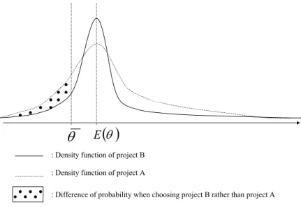
The choice of risk depends on the manager’s reputation. First consider the case of a good-reputation manager. Two effects are at work. Equation (9) shows that effort increases when performance becomes more informative, i.e. the variance σ2pdecreases. Hence, effort has a greater impact on the updated beliefs when a manager opts for project A than when she opts for project B. Therefore, choosing the less risky project implies a higher equilibrium effort which results in a higher cost for the manager. This is the “cost effect”. Next consider the “probability effect”. A good-reputation manager is promoted provided that the updated beliefs E(θ | Π, p, e∗) and the initial
beliefs E(θ) about her talent are similar enough. Thus, this manager prefers the status quo. Hence, she minimizes the variance of E(θ | Π, p, e∗). Equation (11) shows that it induces her to favor the riskier project. The intuition
is the following: If the project is sufficiently risky, it is difficult to infer from its outcome whether success is due to fortune or managerial talent, and whether failure occurs because of bad luck or a lack of managerial skills. Hence the market cannot update precisely its beliefs. Note that both the “cost effect” and the “probability effect” go into the same direction: Opting for B today both decreases the cost of effort incurred by the manager at the equilibrium and maximizes the probability to be promoted tomorrow (see Figure I).
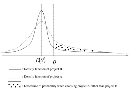
Next, consider the case of a bad-reputation manager. The analysis regarding the “cost effect” parallels the above one: Opting for the riskier project is less costly in terms of effort. Conversely, the analysis regarding the probability of promotion is reversed. If the market’s assessment of the manager’s talent is still bad, the manager is not promoted. Thus, such a manager maximizes var (E(θ | Π, p, e∗)), which imposes, according to (11), to opt for the less risky project (see Figure II).
Insert Figure II: bad-reputation manager here.
Here, the “cost effect” and the “probability effect” go into two opposite directions. Hence, the final choice of the manager depends on the attractiveness of the promotion (i.e. the size of the additional wage ∆). When ∆ ≥ ∆ (E(θ)), with ∆ (E(θ))=d ψ (e∗(A)) − ψ (e∗(B)) Φ ¡ σ2 θ+ σ2B ¢1 2 σ2 θ ¡ θ − E(θ)¢ − Φ ¡ σ2 θ+ σ2A ¢1 2 σ2 θ ¡ θ − E(θ)¢ , (12)
where Φ is the cumulative distribution of N (0, 1), a bad-reputation manager chooses A. Indeed, (12) ensures that the additional wage more than offsets the larger cost incurred by the manager due to her higher effort8.
These results are summarized in the following proposition9.
Proposition 2 Suppose accounting profits are the unique source of information. Then, (i) A manager with a good reputation chooses the riskier project (B),
(ii) A manager with a bad reputation chooses
- the less risky project (A) when ∆ ≥ ∆ (E(θ)) ,
8Alternatively, we could consider the manager’s choice between a more or less ambitious project- more ambitious meaning a higher
expected profit as well as a higher risk. Therefore, choosing the more ambitious project would imply a higher wage in the first period while beliefs would be updated less precisely. Thus, a good-reputation manager would still choose to run a more ambitious project. A bad-reputation manager would still face a trade-off between choosing the less ambitious project in order to increase its probability to be promoted tomorrow or choosing the more ambitious project in order to increase its first period wage and to decrease its cost of effort.
9Notice that the assumption about the observability of the risk of projects is crucial. Indeed, if the risk of project were not
observable the results would be reversed. In equilibrium, a good-reputation manager would prefer the less risky project provided that promotions are sufficiently attractive (conservatism). Conversely, a bad-reputation manager would undertake the riskier project (gambling).
- the riskier project (B) when ∆ < ∆ (E(θ)) .
Observe that ∆ depends on the distance between the updated reputation level of the manager E(θ) and the threshold θ above which the promotion occurs. When this distance is low, a bad-reputation manager has a probability of promotion of about12, whatever the project undertaken. When this distance is high, the probability to be promoted is close to zero, whatever the project carried out. Hence, in these two occasions, the additional wage must be very attractive to induce a bad-reputation manager to opt for A. The threshold ∆ is lower when choosing A rather than B implies a reasonable difference in the probabilities of promotion, that is, when¯¯θ − E(θ)¯¯ takes intermediate values.
That the current reputation E(θ) of a manager drives her risk-taking policy is a direct consequence of the discontinuity in the revenue function we model. Current reputation has no role to play in the standard career concerns model of Holmström [1982, 1999]. This clearly shows up in equation (10), the second term of which would be absent in a traditional model. Since a manager grounds the risk-profile of her action on E(θ), current reputation also influences the level of effort she performs at the equilibrium which, again, differs from the standard career concerns model (the second term of equation (9) would be absent). By contrast, managers only behave to enhance their future- or updated -reputation in standard career concerns settings.
If good, current reputation is an “asset” that must preserved. It can take the form of lowering the level of risk an entrepreneur takes when not defaulting in ones’ commitments vis-a-vis lenders allows to latter obtain debt at better conditions [Diamond, 1998]. In a very different setting, characterized by the observability of the risk-taking policy, we obtain the opposite result.
It is worth explicitly comparing the level of effort performed by a manager depending on whether her reputation is good or bad, when ∆ ≥ ∆ (E(θ)). As shown in (9), there are two effects at work. First, choosing the riskier project leads to lower the level of effort exerted. Second, the farther the manager’s talent from the threshold that allows her to be promoted (i.e. the higher¯¯θ − E(θ)¯¯), the lower the incentives to work. Hence, for a given distance
between the promotion threshold and her reputation, the manager works less when she has a good reputation than when she has a bad reputation since she chooses A in the first case (provided that the promotion is attractive enough), whereas she selects B in the second case. Hence, even though a riskier policy does not directly reduces the expected profitability of the firm, it indirectly lowers this profitability through the level of effort exerted by the manager. Here, being talented induces “laziness” and adversely impacts the profits of the firm. These results are summarized in the following proposition.
Proposition 3 Suppose accounting profits are the unique source of information. Let ∆ ≥ ∆ (E(θ)) and¯¯θ − E(θ)¯¯ be fixed. Then, a manager exerts a higher level of effort if she has a bad rather than a good reputation.
In the next section, we investigate the case where the employer has the opportunity to monitor the manager.
IV. Monitoring as a second source of information
Working backward, we first determine the manager’s choice of effort. Then, we investigate her employer’s level of monitoring. Finally, we analyze the manager’s choice of risk.
IV.A. The Manager’s First-Period Choice of Effort
Suppose that the market anticipates e∗. A manager chooses e so as to maximize her second-period expected
wage less her first-period cost of effort, that is,
E£E£E(θ | Π, τ , p, σ2, e∗)¤¤+ Pr¡E(θ | Π, τ , p, σ2, e∗) ≥ θ¢× ∆ − ψ (e) , (13) where the first expectation is with respect to τ , while the second and the third expectations are with respect to Π and θ, respectively. Now, the market can use a second source of information, namely the public report, to update the manager’s reputation. This naturally influences the manager’s choice of effort as appears in (13). Assuming
an interior solution, the first-order condition for an equilibrium satisfies cov à θ,fbe ¡ Π, τ | p, σ2, e∗¢ b f (Π, τ | p, σ2, e∗) ! + ∂ ∂e © Pr¡E(θ | Π, τ, p, σ2, e∗) ≥ θ¢× ∆ª= ψ0(e∗) . (14) Overall, equation (14) describes the manager’s marginal incentives to exert effort. It reduces to
σ2 θ σ2 θ+ σ2p | {z } T erm 1 + σ 2 θσ2p σ2 θ(σ2p+ σ2) + σ2pσ2 | {z } T erm 2 + v³¡θ − E(θ)¢2, σ2θ, σ2p, σ2´× ∆ | {z } T erm 3 = ψ0(e∗) , (15) where v (.)=d σ 2 p+ σ2 £ σ4 p(σ2θ+ σ2) + 2σ2θσ2pσ2 + ¡ σ2 θ+ σ2p ¢ σ4¤12 ×√1 2πexp " −1 2 ¡ θ − E(θ)¢2¡σ2 θ ¡ σ2 p+ σ2 ¢ + σ2 pσ2 ¢2 σ4 θ £ σ4 p(σ2θ+ σ2) + 2σ2θσ2pσ2 + ¡ σ2 θ+ σ2p ¢ σ4¤ # (16) is decreasing in ¯¯θ − E(θ)¯¯. The first two terms of equation (15) are equal to the covariance of equation (14). Term 1 is identical to the first term in (9) where accounting profits were the unique source of information. Term 2 represents the marginal increase in effort due to the incentives created by the second source of information through the updating process. Term 3 shows the marginal increase in effort created by the additional wage ∆ the manager earns when she is promoted. Term 3 is larger than its corresponding counterpart in (9). The existence of the second source of information reinforces the incentives to work.
IV.B. The Employer’s First-Period Monitoring Decision
By incurring the cost c(σ2), the employer chooses the precision of the report τ he receives. When doing so, the manager is already hired for the first period. This implies that the employer selects the level of monitoring that maximizes the firm’s first-period expected net profits:
E (Π (θ, rp, e∗| p)) − W (E(θ)) − c
¡
σ2¢. (17) The first-order condition of (17) reduces to
∂e∗ ∂σ2 = c0
¡
Let ψ0−1denote the reciprocal function of ψ0. Then, equation (18) reduces to σ2 θσ2p ¡ σ2 θ+ σ2p ¢ £ σ2 θ ¡ σ2 + σ2 p ¢ + σ2σ2 p ¤2 | {z } T erm A −∂v (.) ∂σ2 × ∆ | {z } T erm B × ψ 0−1 Ã σ2 θ σ2 θ+ σ2p + σ 2 θσ2p σ2 θ(σ2p+ σ2) + σ2pσ2 + v (.) ! = −c0¡σ2¢ | {z } >0 . (19)
Term A shows the impact of monitoring on the marginal incentives to exert effort created by the second source of information, that is, the marginal increase of Term 2 (in (15)) when σ2 decreases. Term B shows the impact
of monitoring on the marginal incentives to exert effort created by the additional wage ∆, that is, the marginal increase in Term 3 (in (15)) when σ2 decreases. Overall, the left-hand side of (19) represents the marginal gain of
monitoring for the employer. At the equilibrium, this gain just offsets the monitoring marginal cost −c0¡σ2¢10. Assuming that A exhibits a low level of risk, i.e. σ2
A< σ2(defined in the Appendix) ensures that the marginal
gain of monitoring is higher when a manager opts for B rather than for A (observe that at the limit, i.e. when σ2
A= 0, the marginal gain of monitoring is zero since accounting profits (Π) are a sufficient statistic with respect
to the public report τ when estimating E(θ)). Since the marginal cost of monitoring does not depend on the risk of the project undertaken, we obtain that the employer exerts a higher level of monitoring if a given manager opts for B rather than for A (Part (i) of Proposition 4). When σ2A is low enough, there exists cases where the employer does not exert monitoring. In particular, when ¯¯θ − E(θ)¯¯ takes either low or high values, then, for a finite ∆, the impact of the monitoring on the marginal incentives to exert effort created by the additional wage µ ∂v(θ,E(θ),σ2 θ,σ2p,σ2) ∂σ2 × ∆ ¶
is low so that the marginal cost of monitoring can offset the marginal gain of monitoring.
This case corresponds to Part (ii) of Proposition 4. Proposition 4 Let σ2
A< σ2. For a given manager, the employer:
(i) Exerts a higher monitoring level if this manager has opted for the riskier project (B) rather than for the less risky project (A),
1 0We refer the reader to the Appendix, proof of Proposition 4, for a discussion of the solution given by equation (19) as the global
(ii) Does not resort to monitoring when this manager opts for A, while A implies a low level of risk and the marginal cost of monitoring is equal to the marginal gain of monitoring only when σ2 → +∞.
Finally, we determine the choice of risk by the manager. IV.C. The Manager’s First-Period Choice of Risk
The manager anticipates that the observable choice of risk she makes influences the employer’s level of moni-toring.
A bad-reputation manager still balances the “cost effect” and the “probability effect” when considering her choice of project. Both the “cost effect” and the “probability effect” consist of a direct as well as of an indirect effect. The direct “probability effect” results from the shift from B to A on the probability of promotion. Again, assuming that σ2A < σ2 implies that choosing a less risky project facilitates the learning process so that the direct effect is positive. The indirect “probability effect” corresponds to the positive effect of monitoring on the probability of promotion, times the negative impact of a shift from B to A on the equilibrium level of monitoring. Note that monitoring decreases because its marginal gain (i.e. the increase in managerial effort) is higher when project B rather than project A is chosen, whereas its marginal cost does not depend on the risk of the project. Hence, the indirect “probability effect” is negative. However, it does not offset the positive direct “probability effect” if the marginal cost of monitoring is sufficiently increasing to avoid a large difference between monitoring levels depending on whether A or B was chosen (i.e. c00σ2∗¡σ2
A
¢
) > κ- see in the Appendix -and c000 < 0). To
summarize, opting for A rather than for B increases the probability of promotion for a bad-reputation manager. Next, turn to the “cost effect” which also consists of a direct as well as of an indirect effect. For a given level of monitoring (σ2 6= 0), opting for A (with σ2A < σ2) leads to a large updating of beliefs whereas opting for B (with σ2
B > σ2) leads to a slight updating of beliefs. Hence, exerting effort has a larger impact on the perception
increases the equilibrium level of effort which raises the cost incurred by a bad-reputation manager (direct effect). On the other hand, opting for A decreases the level of monitoring, and monitoring implies less effort. Thus, the indirect “cost effect” is positive for a bad-reputation manager. However, it does not offset the negative impact of a shift from B to A on the cost resulting from e∗ when the marginal cost of monitoring is sufficiently increasing (i.e. c00¡σ2∗¡σ2
A
¢¢
> κ and c000 < 0) to avoid a large difference between monitoring levels depending on whether
A or B was chosen. To summarize, a bad-reputation manager increases her cost of effort when she opts for A rather than for B.
Hence, in the case of a bad-reputation manager, the “cost effect” and the “probability effect” go into two opposite directions. Thus, the bad-reputation manager faces a trade-off between increasing her probability of promotion and reducing the cost of effort she incurs. Overall, she opts for the less risky project when the promotion is sufficiently attractive, that is when ∆ ≥ ∆ (E(θ)), where
∆ (E(θ))=d ψ (e∗(A)) − ψ (e∗(B)) Φ · (θ−E(θ))(σ2 θ(σ2B+σ2(B))+σ2Bσ2(B)) σ2 θ[σ4B(σθ2+σ2(B))+2σ2θσ2Bσ2(B)+(σ2θ+σ2B)σ4(B)] 1 2 ¸ − Φ · (θ−E(θ))(σ2 θ(σ2A+σ2(A))+σ2Aσ2(A)) σ2
θ[σ4A(σθ2+σ2(A))+2σ2θσ2Aσ2(A)+(σ2θ+σ2A)σ4(A)] 1 2
¸ .
When there is no monitoring if the manager opts for A, the threshold becomes ∆0(E(θ)), which is given by the combination of ∆ (E(θ)) and σ2(A) → ∞.
Now consider a manager with a good reputation. As for the “cost effect” and the “probability effect”, the indirect effect is dominated by the direct effect under the same conditions on the cost function and on the level of risk of A and B as above. Both the “cost effect” and the “probability effect” induce the good-reputation manager to opt for the riskier project (B) as when accounting profits were the sole source of information.
4). This implies that for a given ¯¯θ − E(θ)¯¯, the employer monitors more intensely a manager if she has a good reputation than if she has a bad reputation. These results are summarized in the following proposition.
Proposition 5 Let σ2 B> σ2, σ2A< σ2, and ψ000> 0, c000< 0, c00 ¡ σ2∗¡σ2 A ¢¢ > κ. (i) A manager with a good reputation strictly prefers the riskier project (B).
(ii) A manager with a bad reputation strictly prefers the less risky project (A) when ∆ ≥ ∆ (E(θ)) if there is monitoring or ∆ ≥ ∆0(E(θ)) if there is no monitoring when A is realized.
(iii) Let ¯¯θ − E(θ)¯¯ be fixed. Then, the level of monitoring performed by the employer is strictly higher if the manager has a good rather than a bad reputation.
The following results are obtained for more general cost functions c(.), i.e. when the assumptions regarding c00¡σ2∗¡σ2
A
¢¢
and c000 are relaxed, and for a more general cost of effort ψ(.), i.e. when the assumption regarding
ψ000 is relaxed.
Proposition 6 Let σ2B> σ2 and σ2A< σ2.
(i) A manager with a good reputation weakly prefers the riskier project (B).
(ii) A manager with a bad reputation weakly prefers the less risky project (A) when ∆ ≥ ∆ (E(θ)) if there is monitoring or ∆ ≥ ∆0(E(θ)) if there is no monitoring when A is realized.
(iii) Let¯¯θ − E(θ)¯¯ be fixed. Then, the level of monitoring performed by the employer is higher if the manager has a good rather than a bad reputation.
The connection between our results and the theoretical literature is discussed below. IV.D. Related Theoretical Literature
It is insightful to compare our research to papers dealing with risk-taking policy by managers, either in a career concerns context or in an adverse selection context.
When managers privately know their respective ability while their policy with respect to risk (through hedging) is not observable, good managers want the market to learn information regarding their talent. Hence, they hedge because hedging ameliorates the accuracy of the information contained by corporate profits regarding their ability as it eliminates extraneous noise. Conversely, bad managers do not want the market to learn information. Accordingly, they do not hedge [Breeden and Viswanathan11, 1998]. In our model, information is symmetric but
incomplete. This drives the opposite result: A good-reputation manager tries to impede the learning process since she favors the status quo whereas a bad-reputation manager wants to facilitate this process since she wants the market to modify its beliefs.
Now consider the case where managers do not have privileged information regarding their talent and are risk-averse in the sense that they fear to have their wage reassessed. Whatever their talent, that their policy with respect to risk (either through a choice of project or through hedging) is observable, influences the way they impede the updating of beliefs process. This can take the form of a no-hedging policy [DeMarzo and Duffie, 1995] or a high-risk-taking policy [Hermalin, 1993]. We show that this motive still holds for the risk-neutral managers we consider provided they have a good reputation. However, a risk-neutral manager, if her reputation is bad, opts for the less risky projects to facilitate the learning process since the status quo is detrimental to her. A risk-averse bad-reputation manager would make the same decision provided that the increase in expected utility resulting from the higher probability of promotion more than offsets the decrease in expected utility resulting from the higher probability of having her wage lowered as the aftermath of a poor outcome.
Moreover, what also differentiates our research from the above papers is that we analyze the impact of the risk-taking policy on the incentives to exert effort. Specifically, we show that because a good-reputation manager impedes the learning process by favoring risk, this induces her to lower the level of effort she exerts. Hence, the mechanism through which the profitability of firms is adversely impacted is different from what Hermalin
1 1As for managers lying in the intermediate ability-range, the results are mixed. Besides, Breeden and Viswanathan [1998] show
considers: He simply assumes that the managers’ and the employers’ interests pertaining to the risk-taking policy may not be aligned, while we show that risk-taking indirectly decreases profitability.
Finally, we investigate how the employer resorts to monitoring, especially when a good-reputation manager tries to impede the updating process. This second source of information is absent in Hermalin [1993], DeMarzo and Duffie [1995], and Breeden and Viswanathan [1998]. It allows us to propose original implications.
IV.E. Implications
The implications we can derive from the framework we adopt here go beyond the “promotion” interpretation we developed in a managerial context. They include the following.
Consider the case of an engineer working in a R&D department and on the eve of creating her own firm. A good reputation is a necessary condition to obtain the funds she needs to establish her future company because of credit-rationing. Hence, in order to keep her good reputation, the engineer undertakes very risky projects or follows high-risk strategies to reach the objective she has been assigned. Her head of department can observe this behavior. In such a case, her reaction could be to intensify his monitoring activity (by organizing more meetings and so forth) which would positively impact the accuracy of his assessment of the engineer’s input. Monitoring of a lower-reputation manager would be less necessary.
In the venture capital industry, general partners (venture capitalists) periodically seek financial contributions from limited partners (e.g. mutual or pension funds) to set up new funds. The better their reputation, the higher the management fees or the larger the carried interest general partners are able to bargain. Thus, setting up a new fund can imply a substantial increase in revenue for the general partners. To prevent the market from updating its beliefs regarding their talent, they can increase the risk of the projects the current fund they run invests in: For example, they select a high proportion of early-stage ventures they allocate money to. This risk is observable. A possible reaction from the limited partners is to bargain for more seats on the advisory board so
as to better monitor the investments or to resort to gatekeepers.
In the same vein, a divisional manager may benefit from launching ambitious programs of investment (more perks and fame associated to the growth in the size of the division). So as to keep her good reputation, she can undertake very risky ventures (e.g. enter emerging markets) before the headquarters makes the internal allocation of resources decision. The latter can assess the riskiness of the venture thanks to his experience. He can obtain more accurate and less manipulable information by carving out the division so that it is listed on the stock exchange which ensures analysts will assess its performance.
Finally, let us consider the mutual fund industry. Risk-taking policies are observable by insiders; managers in charge of a sector fund are likely to behave to obtain a promotion in the form of managing a growth or a growth and income fund, and reputation plays an important role12. It would be of interest to test how a manager does alter the riskiness of the assets she holds when she has this perspective of much larger revenues. Does she lock-in her reputation by increasing the risk of her portfolio when she feels confident about her “promotion”? The portfolio manager can achieve such a riskier profile either by turning over some of her existing security holdings or, if allowed, by altering the entire fund synthetically with derivative positions. And does she let the market learn more information regarding her talent, through the achievement of a less risky portfolio when she feels her reputation will not allow her to get the kind of promotion we consider? Tests [e.g. Chevalier and Ellison, 1997] have been recently conducted that bear some resemblance with the one we suggest: Broadly speaking, they examine the reaction of mutual funds in terms of risk-taking policy to their position with respect to the market index at an interim date in a context where the cash inflows of the coming year from investors respond to end-of-year publicly announced profits (or losses), which constitutes implicit incentives. However, these studies investigate the case of outside investors unable to distinguish between various risk-taking policies which does not fit with our assumption. It would be worth considering the career concerns of managers when their choice of risk
1 2For example, Chevalier and Ellison [1997] show that the cash inflows from investors positively respond to the termination of
is observable, as is the case by insiders within the fund. Moreover, they examine “routine” incentives derived from investors’ inflows whereas we consider incentives derived from the opportunity to “hit the jackpot”. In this respect, our approach is more similar to Chevalier and Ellison [1999] who examine the risk-taking incentives of mutual fund managers who fear losing their jobs. However, Chevalier and Ellison [1999] test herding issues. Furthermore, they consider young and old managers, not good and bad ones13.
In the next section, we endogenize the threshold against which managers compete.
V. Competition between Two Managers For One Position
We depart from the previous model in the sense that, here, two managers, i and −i, who know each other’s reputation compete for one position in the second period. We restrict our attention to the role of accounting profits- as in Section III -and leave aside the report that would result from monitoring. The manager with the better updated reputation is promoted at the beginning of the second period. Hence, manager i is promoted if and only if
E(θi| Πi, pi, e∗i) ≥ E(θ−i| Π−i, p−i, e∗−i). (20)
Then, she gets the additional wage ∆.
V.A. Manager i’s First-Period Choice of effort
Suppose that the market anticipates the equilibrium efforts e∗
i, e∗−i. Manager i chooses e∗i so as to maximize14
E [E(θi| Πi, pi, e∗i)] + Pr
¡
E(θi| Πi, pi, e∗i) ≥ E(θ−i| Π−i, p−i, e∗−i)
¢
× ∆ − ψ (ei) . (21)
Observe that the threshold above which i is promoted is now endogenous: It depends on her opponent’s updated reputation which appears in the second term in (21). Assuming an interior solution, the first-order condition for
1 3Although it is likely there exists a survival bias so that older managers are on average more talented than younger ones, what
mostly distinguishes older managers from younger ones is the precision regarding their ability: The talent of older managers being assessed with a higher precision than the talent of younger ones.
1 4In the case where a non competitive labor market is considered, the manager gets w if she is not promoted and w + ∆ if she is
an equilibrium reduces to cov à θi, b fe∗ i b f ! +∂ Pr ¡
E(θi| Πi, pi, e∗i) ≥ E((θ−i| Π−i, p−i, e∗−i)
¢
∂ei × ∆ = ψ 0(e∗
i) . (22)
Computing at e−i= e∗
−i leads to the equilibrium and optimal level of effort exerted by manager i. It verifies
σ2 θi σ2 θi+ σ 2 pi + (23) ∆ µ σ2 θi+σ2pi σ2 θi ¶ µ σ4 θi σ2 θi+σ2pi + σ4 θ−i σ2 θ−i+σ2p−i ¶1 2 1 √ 2πexp − 1 2
(E(θ−i) − E(θi))2 σ4 θi σ2 θi+σ2pi + σ4 θ−i σ2 θ−i+σ2p−i = ψ0(e∗i) .
Here, manager i grounds her effort decision on (E(θ−i) − E(θi))2 which represents the difference between her
reputation and the reputation of her opponent, rather than against an exogenous benchmark. The larger (E(θ−i) − E(θi))2, the lower the incentives to exert effort. Indeed, as (E(θ−i) − E(θi))2 increases, the impact
that effort has on the probability to have a better reputation than one’s opponent decreases. Manager i also bases her effort decision on σ
4 θ−i
σ2
θ−i+σ2p−i which depends on the uncertainty regarding her opponent’s talent and on
the choice of project the latter takes.
Now, consider the choices the two managers take regarding risk. V.B. Manager i’s First-Period Choice of risk
As in the above sections, manager i chooses the risk-profile of the project she undertakes by considering both the cost of effort and the probability of promotion it implies. Minimizing the cost of effort still implies to maximize the project’s risk.
Let the contest have a favorite and an outsider in the sense that E(θf) > E(θo). Their actions or characteristics
are denoted by f and o, respectively.
her probability of promotion, Pr (E((θf| Πf, pf, e∗f)) ≥ E(θo| Πo, po, e∗o)) = 1 − Φ E(θo) − E(θf ) ³ σ4 θf σ2 θf+σ2pf + σ4 θo σ2 θo+σ2po ´1 2 , by setting σ2
pf as high as possible, i.e. by choosing B. Hence, the cost effect and the probability effect go into the
same direction: The manager who enjoys the better reputation has a dominant strategy which consists in opting for the riskier project.
Now consider the outsider’s decision. The outsider anticipates the favorite’s choice of B. She maximizes the probability of promotion when minimizing σ2po. However, opting for A implies a higher cost of effort. Hence, she
faces a trade-off similar to the one studied in Section III. The outsider chooses the less risky project A when the additional wage ∆ is attractive enough, i.e. ∆ ≥ ∆ (E(θf), E(θo)), with
∆ (E(θf), E(θo))=d ψ (e∗ o(A)) − ψ (e∗o(B)) Φ s E(θo)−E(θf) σ4 θf σ2 θf+σ2B + σ4θo σ2 θo+σ2B − Φ s E(θo)−E(θf) σ4 θf σ2 θf+σ2B + σ4θo σ2 θo+σ2A . (24)
Observe that when the favorite’s talent is quite uncertain, i.e. σ2
θf is high, the denominator of (24) is close to
zero so that choosing A or B has a small impact on the outsider’s probability of promotion. Therefore, unless the additional wage is very attractive, the outsider also undertakes project B since it implies less effort.
Proposition 7 Suppose accounting profits are the unique source of information. Then, (i) The manager with the better reputation chooses the riskier project (B),
(ii) The manager with the worse reputation chooses
- the less risky project (A) when ∆ ≥ ∆ (E(θo), E(θf)) ,
- the riskier project (B) when ∆ < ∆ (E(θo), E(θf)) .
V.C. Related Literature and Discussion
The framework we have adopted in this section bears some resemblance with a tournament15: The winner
(here, the promoted manager) gets a reward (here, the additional wage due to the higher productivity). However, major differences remain as promotions are based on the updated assessment of the managers’ talent in our setting whereas there are based on realized output in a standard tournament, which can lead to opposite outcomes. Yet, the relation with models of tournament deserves some comments. In particular, this theoretical literature has recently investigated the risk-taking behaviors of players in multi-period settings. Consistent with conventional wisdom, the winner at an interim stage chooses a safer strategy than the laggard, thus formalizing the sports’ intuition that the laggard has “nothing to lose”, and consequently gambles while the winner wants to secure his position. This is true for R&D competition between two firms which strategically choose the level of variance of their projects as a function of their relative positioning in the race they run [Cabral, 2002]. The idea that players lagging behind at an interim stage are less conservative than interim winners is pervasive. As argued by Brown, Harlow and Starks [1996], competition between firms in the mutual fund industry can be viewed as a tournament. Models of such tournaments [e.g. Goriaev, Palomino, and Prat, 2002], where ranking has a strong impact on fund flows, obtain this pattern16.
We derive the unambiguous opposite and new result when the level of risk actually chosen by the players is observable: The laggard takes few risks (provided the attractiveness of the promotion is high enough), whereas the interim winner takes a lot of risks17.
1 5Seminal papers include Lazear and Rosen [1981], Green and Stockey [1983], Nalebuff and Stiglitz [1983], and Malcomson [1984]. 1 6Empirical tests pertaining to the mutual fund tournament hypothesis have been recently performed. The first results that interim
losers gamble to catch up to the interim winners whereas the latter index to secure their position [Brown, Harlow and Starks, 1996, Koshi and Pontiff, 1999] must be taken cautiously as they may be plagued by auto- and cross-correlation of the funds’ returns. When these two problems are taken into account, there is no more evidence of these patterns [Busse, 2001]. When cross-correlation alone is taken into account, the patterns described above hold [Goriaev, Palomino and Prat, 2002]. However, outside investors are unable to distinguish between various risk-taking policies which does not fit with our assumption. Again, it would be worth considering the career concerns of managers when their choice of risk is observable, as is the case by insiders. Moreover, only “routine” incentives derived from investors’ inflows are investigated whereas we consider incentives derived from the opportunity to “hit the jackpot”.
1 7Taylor [2001], in a mutual fund industry tournament setting, derives a mixed strategy equilibrium where “winning managers are
more likely to choose a risky portfolio than losing managers” as he put it. However, he obtains this result because increasing risk also increases the expected return of a portfolio- whereas all parties are risk-neutral- which induces winning managers to take more risk than the index although its decreases the probability of a victory.
When homogenous players compete in a tournament with risk an effort as choice variables, they indulge in excessive risk-taking because it allows them so save on effort costs as effort then has little if no impact on the outcome [Hvide, 2000]. The discontinuity in the revue function of the players resulting from the tournament structure plays no rule in the choice of risk, which differs from the result obtained here.
Finally, note that the tournament-like setting of this section seems particularly relevant to the competition between managers at higher levels in the hierarchy- presumably older managers -than the setting we adopted in the previous sections where each manager was competing against an exogenous benchmark. Indeed, as they progress in the hierarchy, managers are more likely to identify the few opponents they compete with.
VI. Concluding Remarks
The perspective of a substantial increase in revenue that we model as a discontinuity in the revenue function may not discipline managers that have a good reputation to keep when their risk-taking policy is observable. The latter select risky actions to impede the learning process regarding their talents. As this learning process is impaired, these managers are not induced to perform high levels of effort. Conversely, bad-reputation managers are willing to let the market learn more information regarding their talents, provided that the attractiveness of the promotion is high. Hence, they favor less risky projects. We examine a possible reaction of their current employer: Resorting to a source of information the precision of which is not manipulable by the managers facilitates the updating of beliefs process. However, costly monitoring is not always desirable when managers choose the less risky project. Interestingly, the result that an interim-winner manager opts for the riskier project whereas an interim-loser manager opts for the less risky project still holds when two managers of heterogeneous reputation compete for one position at a higher level. This goes against the conventional wisdom that laggards have nothing to lose and then gamble.
Appendix
Profits as the unique source of information
Working backward, we first determine the choice of effort by the manager. A. Proof of Proposition 1
Suppose that the market anticipates the equilibrium effort e∗. The manager chooses e so as to maximize
E [E(θ | Π, p, e∗)] + Pr¡E(θ | Π, p, e∗) ≥ θ¢× ∆ − ψ (e) , (25) where the first expectation is with respect to Π, the second expectation is with respect to θ, and
Π = θ + rp+ e. (26)
Assuming an interior solution, the first-order condition for an equilibrium is
∂ ∂e "Z ÃZ θf (θ, Π | p, e ∗) b f (Π | p, e∗) dθ ! d bF (Π | p, e) + Pr¡E(θ | Π, p, e∗) ≥ θ¢× ∆ #¯¯ ¯ ¯ ¯e=e∗ = ψ0(e∗) , (27) or Z Z θfbe(Π | p, e ∗) b f (Π | p, e∗)f (θ, Π | p, e ∗) dΠdθ +∂ Pr ¡ E(θ | Π, p, e∗) ≥ θ¢ ∂e × ∆ = ψ 0(e∗) , (28) where f (Π | ) =b Z f (Π, θ | ) dθ (29) and f (Π, θ | ) denote respectively the marginal density of the observables, and the joint density of the talent and of the observables, given the equilibrium level of effort e∗and the choice of project p. bf
edenotes the derivative of
the marginal distribution with respect to effort.
Consider the first term in the left-hand side of (28). Since the likelihood ratio has zero mean, i.e. E à b fe b f ! = 0, Z Z θfbe(Π | p, e ∗) b f (Π | p, e∗)f (θ, Π | p, e ∗) dΠ 1dθ = cov à θ,fbe b f ! . (30)
The marginal density bf (Π | p, e∗) is proportional to exp à −1 2 (Π − (E(θ) + e))2 σ2 θ+ σ2p ! and b fe(.) b f (.) = (θ − E(θ)) + rp σ2 θ+ σ2p . (31) Thus, cov à θ,fbe b f ! = σ 2 θ σ2 θ+ σ2p . (32)
Now turn to the second part in the left-hand side of (28). Applying statistic rules for computing a conditional expectation in the case of normal laws gives
E(θ | Π, p, e∗) = E(θ) + σ 2 θ σ2 θ+ σ2p(Π − E(Π)) , (33) which leads to Pr¡E(θ | Π, p, e∗) ≥ θ¢= 1 − Φ ¡ θ − E(θ)¢+ σ2θ σ2 θ+σ2p(e ∗− e) σ2 θ (σ2 θ+σ2p) 1 2 . (34) Thus, ∂ Pr¡E(θ | Π, p, e∗) ≥ θ¢ ∂e ¯ ¯ ¯ ¯ ¯ e=e∗ =¡ 1 σ2 θ+ σ2p ¢1 2 1 √ 2πexp " −1 2 ¡ θ − E(θ)¢2¡σ2 θ+ σ2p ¢ σ4 θ # . (35) Combining (32) and (35), and rearranging shows that the manager exerts an effort e∗ that verifies
σ2 θ σ2 θ+ σ2p +¡ ∆ σ2 θ+ σ2p ¢1 2 1 √ 2πexp " −1 2 ¡ θ − E(θ)¢2¡σ2 θ+ σ2p ¢ σ4 θ # = ψ0(e∗) . (36) B. Proof of Proposition 2
The managers chooses p so as to maximize
E [E(θ | Π, p, e∗)] + Pr¡E(θ | Π, p, e∗) ≥ θ¢× ∆ − ψ (e∗) . (37) She leaves aside E [E(θ | Π, p, e∗)] since at the equilibrium the market perfectly anticipates e∗ and observes the
choice of project, so that
Hence, the manager makes her risk decision by considering the cost of effort implied by the project and the probability to be promoted.
Consider a good-reputation manager. First, (36) shows that minimizing the cost of effort implies to maximize σ2p. Next, examine the probability of promotion: Using statistic rules for computing conditional expectations in
the case of normal laws leads to E(θ | Π, p, e∗) ∼ N
µ E(θ); σ 4 θ σ2 θ+ σ2p ¶ . Thus, raising σ2
p decreases the variance of
E(θ | Π, p, e∗) and in turn maximizes the probability to be above the threshold θ as E(θ) ≥ θ. Hence, overall, a good-reputation manager opts for B.
Now consider a bad-reputation manager. Since E(θ) < θ, she maximizes her probability of promotion when minimizing σ2
p. However, minimizing σ2pimplies a higher cost of effort. Hence, the trade-off she faces. She chooses
A when · −ψ (e∗(A)) + Pr¡E(θ | Π, A, e∗) ≥ θ¢× ∆ ¸ ≥ · −ψ (e∗(B)) + Pr¡E(θ | Π, B, e∗) ≥ θ¢× ∆ ¸ , (39) which imposes that the additional wage ∆ is attractive enough: ∆ ≥ ∆ (E(θ)) , with
∆ (E(θ))=d ψ (e∗(A)) − ψ (e∗(B)) Φ ¡θ − E(θ)¢ ¡ σ2 θ+ σ2B ¢1 2 σ2 θ − Φ ¡θ − E(θ)¢ ¡ σ2 θ+ σ2A ¢1 2 σ2 θ . (40)
The report as a second source of information
First, we determine the equilibrium effort e∗. Suppose that the market anticipates e∗. The manager chooses e so as to maximize
E£E£E(θ | Π, τ , p, σ2, e∗)¤¤+ Pr¡E(θ | Π, τ , p, σ2, e∗) ≥ θ¢× ∆ − ψ (e) , (41) where the first expectation of the first term in (41) is with respect to τ , while the second and the third expectations are with respect to Π and θ, respectively. Assuming an interior solution, the first-order condition for an equilibrium