aCentre Urbanisation Culture Société, Institut national de la recherche scientifique, 385 Sherbrooke Street East, Montréal, Québec H2X 1E3, Canada bDepartment of Kinesiology, University of Montreal, Montreal, QC H3C 3J7, Canada
cGeoHealth Laboratory, Department of Geography, University of Canterbury, Private Bag 4800, Christchurch 8140, New Zealand
A R T I C L E I N F O Keywords: Cycling Noise Air Pollution Transport
Geographic Information Systems
A B S T R A C T
According to the World Health Organization, air pollution and road traffic noise are two important environ-mental nuisances that could be harmful to the health and well-being of urban populations. Earlier studies suggest that motorists are more exposed to air pollutants than are active transportation users. However, because of their level of physical activity, cyclists also inhale more air pollutants. The main objective of this paper is to measure individuals' levels of exposure to air pollution (nitrogen dioxide– NO2) and road traffic noise according to their
use of different modes of transportation.
Three teams of three people each were formed: one person would travel by bicycle, one by public transit, and the third by car. Nearly one hundred trips were made, from various outlying Montreal neighbourhoods to the downtown area at 8 am, and in the opposite direction at 5 pm.
The use of mixed models demonstrated that public transit commuters' and cyclists' levels of exposure to noise are significantly greater than motorists' exposure. Again, using mixed models, we found that although the levels of exposure to the NO2pollutant do not significantly differ among the three modes, the inhaled doses of NO2
pollutant are more than three times higher for cyclists than for motorists due to their stronger ventilation rate. It is hardly surprising that the benefits of physical activity are of course greater for cyclists: they burn 3.63 times more calories than motorists. This ratio is also higher for public transport users (1.73) who combine several modes (walking, bus and/or subway and walking).
1. Introduction
The concentrations of air pollutants and level of traffic noise gen-erated by road transportation represent a major public health issue (Kim et al., 2012;Zuurbier et al., 2010). Aware of the problems caused by road traffic in terms of the quality of life and health of individuals living in urban environments, authorities in many cities around the world have focused on developing networks of bicycle paths to reduce the dependence on cars. In this regard, according to a 2013 survey conducted by the City of Montreal, there was a nearly 60% increase in the number of bicycle trips since 2008 (Ville de Montréal, 2017). Many factors have contributed to this increase in the modal share of cycling, especially in central neighbourhoods on the Island of Montreal. For example, over the past twenty-five years (1991–2016), the Island of Montreal cycling network was expanded from 270 km to 732 km (Houde et al., 2018), and in 2009 a bike sharing system was set up in Montreal, and the number of stations as well as the number of bicycles have continually grown up to the present time. Despite these efforts
made to encourage the practice of bicycling in the City of Montreal, cycling still has a relatively low mode share for commuting, compared with the car and public transit (3.9%, compared with 50.1% and 36.5%, according to Statistics Canada data for 2016).
The period of the rush-hour commute constitutes a micro-environ-ment that is very interesting to study regarding exposure to air pollu-tants and road traffic noise, given the high levels and pollution peaks, measured at these times of the day (Laumbach et al., 2015). In addition this is a time of day many people are travelling and it has been shown to have the potential to disproportionately contribute to an individuals' daily exposure (Hill and Gooch, 2007). Comparisons of the levels of exposure to pollutants with various modes of transportation—mainly by car, public transit, and cycling—have been made in a number of cities, particularly: Sydney for nitrogen dioxide (NO2) (Chertok et al.,
2004), Barcelona for carbon monoxide (CO) and PM2.5particles (De
Nazelle et al., 2012), New Delhi for PM2.5(Goel et al., 2015), Athens for
CO (Duci et al., 2003), Stockholm for NO2 (Lewne et al., 2006),
Shanghai for PM2.5(Liu et al., 2015), London for PM2.5(Kaur et al.,
https://doi.org/10.1016/j.jtrangeo.2018.06.007
Received 22 December 2017; Received in revised form 7 June 2018; Accepted 8 June 2018
⁎Corresponding author.
E-mail address:philippe.apparicio@ucs.inrs.ca(P. Apparicio).
2005),Beijing for CO and PM2.5(Huang et al., 2012;Yan et al., 2015),
Forshan (China) for PM2.5(Wu et al., 2013), Dublin for PM2.5and PM10
(Nyhan et al., 2014), Arnhem (the Netherlands) (Zuurbier et al., 2010), and Santiago (Chile) for PM2.5(Suárez et al., 2014). In a recent
sys-tematic review of 39 studies comparing exposure to and inhalation of air pollutants with different modes of transportation, Cepeda et al. (2017) conclude that motorists and public transit commuters have higher levels of exposure than cyclists and pedestrians. However, be-cause of their higher levels of ventilation, cyclists followed by pedes-trians may, depending on individual respiration rates, inhale more pollutants. On the other hand, to our knowledge, there have been no studies attempting to compare exposure to noise during rush hours according to the mode of transportation.
The main objective of this study is therefore to measure individuals' levels of exposure to air pollution and road traffic noise during rush hours in Montreal, according to three modes of transportation (car, cycling, and public transit). More specifically, the aim is to meet the following research sub-objectives: 1) compare travel times for rush-hour trips to or from the downtown area using three modes of trans-portation (car, cycling, public transit); 2) compare the levels of ex-posure to noise and air pollution; and 3) compare the doses of pollu-tants inhaled during the trips and the levels of physical activity.
2. Methods
2.1. Study design and routes
Eight urban studies students—four women (aged 21 to 28) and four men (aged 24 to 32)—and a professor in charge of the project (age 43) made the trips in mid-June 2016. Three teams of three people each were formed: one person travelled by bicycle, one by public transit, and the third by car. Each participant kept the same mode of transportation throughout the period. Due to the high summertime temperatures (mean = 28.7 °C; sd = 4.3), the trips by car were made with the win-dows open (without controlled ventilation settings). The trips were made from various outlying Montreal neighbourhoods to the downtown area at 8 am, and in the opposite direction at 5 pm.
Eighteen round trips of approximately ten kilometres each way had previously been selected using Google Maps. A total of 108 trips were thus made (18 × 2 trips (1 trip each way) × 3 modes of transportation). The destinations selected downtown are either centres of higher education—Concordia University, INRS Urbanisation Culture Société, McGill University, and Université du Québec à Montréal—or important employment centres such as the Stock Exchange Tower and Complexe Guy-Favreau (government services and shopping complex) (Fig. 1). The origins of the trips correspond to the intersection of two residential streets in outlying Montreal boroughs, particularly Ahuntsic –Cartier-ville, Rosemont–La Petite-Patrie, Montréal-Nord, Verdun, Saint-Laurent, etc. The members—motorists, cyclists and public transit commuters—of each of the three teams started their trips at exactly the same time. Also, the participants had a Google Maps route sent to them on their portable phones so that they would make the fastest possible trip with their mode of transport.
After cleaning up the data (elimination of trips not made or trips uncompleted due to rain), 99 trips were retained, representing nearly 65 h and more than 1000 km collected on the Island of Montreal (Table 1). It should be noted that some trips were also excluded due to improper use of a device by one of the participants or because of a defective device. In concrete terms, for a given team, if one of the participants (the cyclist, for example) did not have a value for a par-ticular device (e.g. the noise dosimeter), the trips of the other two members of the team (the motorist and the public transit commuter) were also eliminated. In short, 99 valid trips were made, 93 were re-tained in order to measure noise, 60 to measure exposure to air pol-lution, and 54 to measure the participants' heart rate (Fig. 2).
2.2. Measurements of individual exposure
Data collection was based on the use of three types of devices: 1) nine Aeroqual Series 500 Portable Air Quality Sensors, 2) nine Brüel & Kjaer Personal Noise Dose Meters (Type 4448), and 3) nine Garmin GPS watches (910 XT). All the participants retained the same devices throughout the collection period. We used these devices to measure the individuals' exposure to air pollution (NO2) and noise (dB(A)) as well as
their heart rates, and to obtain a GPS trace of the trip. The Aeroqual devices have two sensors—nitrogen dioxide (NO2) and temperature and
humidity sensors—that record the average NO2 value (μg/m3), the
temperature in degrees Celsius, and the percentage of humidity every minute. According to the Aeroqual supplier's product information, the NO2 sensor has the following characteristics: range (0–1 ppm),
minimum detection (0.005 ppm), accuracy of factory calibration (< ± 0.02 ppm 0–0.2 ppm; < ± 10% 0.2–1 ppm), and resolution (0.001 ppm). The Brüel & Kjaer devices record the average decibel le-vels (dB(A)) every minute (Laeq 1 min.). As recommended by the manufacturer, all Personal Noise Dose Meters (Type 4448) were cali-brated once a day using the Sound Calibrator Type 4231.
In order to estimate the inhalation or uptake pollutant dose, wefirst need to obtain a measure of ventilation (breathing parameter). We then simply multiply the measure of exposure to the pollutant by the minute ventilation value (VE). To do this, two methodological approaches are generally employed.
Thefirst consists in setting the ventilation values for each mode for all the trips (Dirks et al., 2012;Dons et al., 2012;Huang et al., 2012). The United States Environmental Protection Agency provides a whole series of values for inhalation rates by age group, sex, and level of ac-tivity (U.S.EPA, 2011), which can then be used (Huang et al., 2012). Similarly, based on theAllan and Richardson (1998)andPanis et al. (2010), Dons et al. (2012)set ventilation values per minute in con-sidering the type of activity (home-based activities, sleep, work, etc.), the mode of transportation (car driver, car passenger, by bike, on foot, by bus, etc.), and the sex.
The second approach involves varying the inhalation rates throughout the trip by equipping the participants with devices to measure, in real time, either their heart rate (Nyhan et al., 2014) or their energy expenditure using an accelerometer (De Nazelle et al., 2012), based on which one can estimate ventilation, or, instead, to directly measure ventilation with a portable cardiopulmonary indirect breath-by-breath calorimetry system (Panis et al., 2010). For example, Nyhan et al. (2014)use heart rate monitors (Actiheart®) to obtain heart rate values that vary throughout the trip. Then, to obtain a measure of ventilation, they use the regression equations obtained by Zuurbier et al. (2009)between ventilation (dependent variable) and heart rate (independent variable) for 34 individuals who had performed a sub-maximal test on a bicycle ergometer (during the physical test, the minute ventilation, breathing frequency and tidal volume were mea-sured using a pneumotachometer, and the heart rates were recorded with Polar RS400 heart rate monitors). Finally, it is worth noting that Dons et al. (2017)have recently proposed an interesting comparison of several methods of estimating the inhaled dose of pollutant using wearable sensors.
The approach used here to precisely estimate ventilation and the inhaled dose of NO2throughout the trips is very similar to that
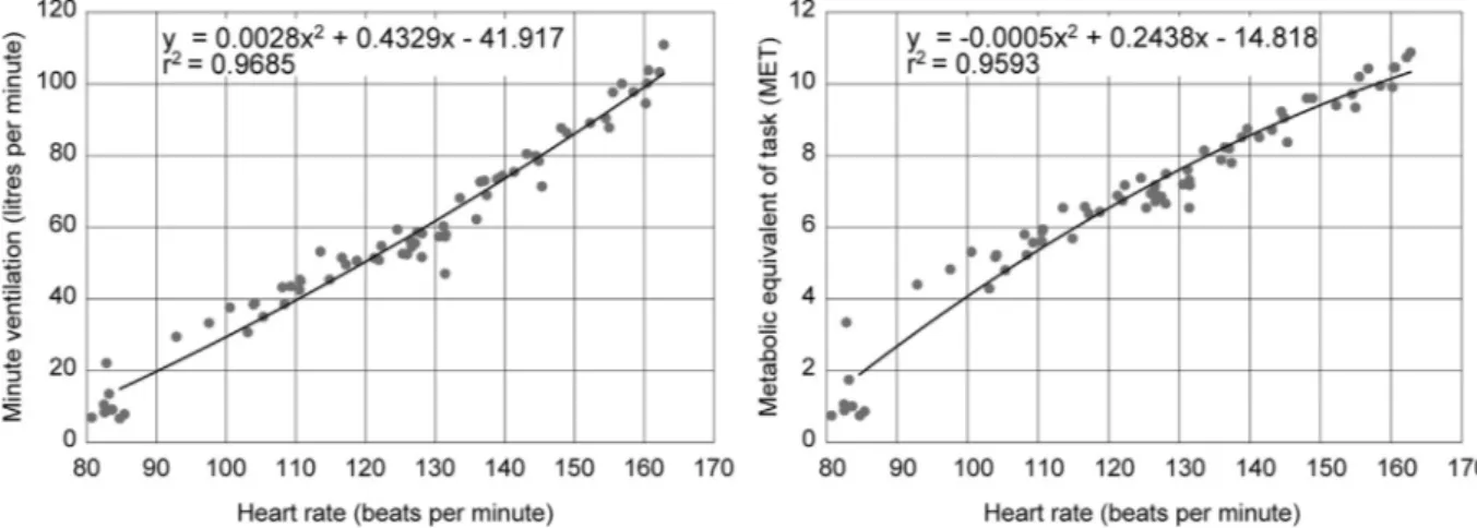
em-ployed byZuurbier et al. (2009). Each participant performed a pro-gressive, continuous and maximal effort test at the Physical Activity and Health Laboratory using the Garmin Forerunner 920XT heart rate monitor watch. The raw heart rate data obtained with the Garmin watch were averaged over 15 s using the MATLAB spline interpolation technique (MathWorks, 2018) in order tofill in the missing data. The metabolic parameters [ventilation rate, minute ventilation, oxygen consumption, and metabolic equivalents (METs)] were measured by indirect calorimetry (MOXUS, Model S-3A, AEI Technologies, PA, USA). The protocol included measures at rest (5 min per position—lying,
sitting, standing) and using progressive effort with increments equiva-lent to 1 MET (i.e. 3.5 ml of oxygen per kg of body weight per minute) every 2 min on the Lode - Corival bicycle ergometer and the Quinton Q65 Series 90 treadmill for other modes of transportation. A 5-min bout
at the intensity corresponding to the target zone for the subject's mode of travel was integrated into the test. Two individualized equations (with a polynomial function) with ventilation and the METs (metabolic equivalent of tasks) as dependent variables and the heart rate as the Fig. 1. Study area and sample routes.
independent variable are then obtained for each participant (Fig. 3). For seven of the nine individuals, the models are very effective, as the R2values are above 0.90; whereas, for two individuals, the equations vary from 0.63 to 0.87. The regression equations are used to estimate ventilation and the METs during the trips based on the heart rate measured with the Garmin watch. Finally, by simply multiplying the estimated ventilation (litres per minute) and the value for the con-centration of the NO2pollutant measured with the Aeroqual sensor, one
can relatively precisely estimate the inhaled dose (I) in micrograms of NO2every minute:
= ∗ ∗
I (VE0.001) NO2
where VE is the ventilation (litres per minute) and NO2is the measure
of concentration (expressed inμg/m3).
Also, for each participant, the caloric expenditure for each one-minute segment is estimated as follows: Calories = 0.0175 (kcal/kg/ min) × weight (kg × METs × (time (min)/3600). Finally, by adding
this up for all the minutes of the trip, we obtain the inhaled dose and caloric expenditure for the entire trip.
2.3. Statistical analyses
Three types of statistical analyses are conducted using the R soft-ware (RCore Team, 2017). First, summary statistics are reported to describe: 1) the trips (route length and duration); 2) the levels of in-dividual exposure to noise and air pollution per minute, and inhalation and respiratory parameters along the trips; and 3) the total inhaled dose and caloric expenditure during the trips for the three modes of trans-portation used.
Second, to determine whether the travel times, the two levels of exposure (NO2and dB(A)), and the four individual measures (heart
rate, ventilation, METs and inhaled dose of the NO2 pollutant) are
significantly different for the three modes, ANOVAs were conducted, as well as Kruskal-Wallis and Tukey tests. Boxplots and violin plots are used to graphically illustrate these differences. Moreover, as Briggs et al. (2008)had done, for each exposure and inhalation variable, two ratios were computed: mean ratios and geometric ratios between cy-clists, public transit commuters, and car commuters.
Third, six linear mixed-effects models are also performed, using the lme4 package in R (Bates et al., 2015), with the two measures of ex-posure (NO2and dB(A)) and the four individual measures (heart rate,
ventilation, METs and inhaled dose of the NO2pollutant) as dependent
variables and the modes of transportation (fixed effects) and the par-ticipants (random effects) as independent variables. There are a number of reasons for using this type of model. We took multiple measures per subject (9 participants). Consequently, the values obtained may vary according to the participants' physiological characteristics. At an equal level of intensity of physical exercise and NO2exposure, the
partici-pants do not have the same levels of heart and ventilation rates and thus of the inhaled dose of pollutant (due to their different ages, sexes and physical conditions). Moreover, the individuals' measures of exposure (NO2and dB(A)) may vary slightly with the particular device assigned
to each participant during the collection period. For example, as men-tioned above, the accuracy of factory calibration of the NO2 sensor
is < ± 10%. Using a mixed model then also enables one to consider the participants' physiological differences and the differences in the sensors used by assuming different random intercepts for each participant. In Table 1
Summary statistics for the 99 trips.
Min Q1 Mean Median Q3 Max SD Sum
Car (N = 33) Route length (km) 5.766 8.031 10.638 9.869 12.337 19.973 3.596 351 Route duration (min) 20.77 25.82 37.66 34.70 49.82 59.73 12.79 1243 Bicycle (N = 33) Route length (km) 5.747 7.606 10.302 10.197 11.863 20.839 3.681 340 Route duration (min) 19.48 28.72 38.44 34.60 45.00 89.20 15.20 1268 Public transit (N = 33) Route length (km) 5.991 7.462 11.195 11.424 14.143 20.843 3.954 369 Route duration (min) 26.43 30.95 41.60 39.27 50.02 73.27 11.40 1373
Min: minimum; Max: maximum; Q1: first quartile; Q3: third quartile; SD: standard deviation.
other words, we add random effects for the nine participants to the fixed effects (modes of transportation). In short, this approach allows one to conduct a nested ANOVA which controls the effect of the par-ticipants and of the precision of the sensors assigned to each.
We compared model fits using the Akaike information criterion (AIC), the Bayesian information criterion (BIC), and the pseudo R2. This
last measure is simply the correlation squared between the Y predicted by the model and the Y observed. For each model, we also computed the intra-class correlation (ICC) as follows:
= +
ICC σ /(σu2 2u σ )e2
where the variance parametersσu2andσe2represent the
between-par-ticipant and within-parbetween-par-ticipant variances, respectively. This coefficient measures the proportion of the variance of the dependent variable be-tween participants.
3. Results
3.1. Comparison of travel times for the trips by mode of transportation Out of the 33 trips made, motorists arrivedfirst 16 times (48.5%), compared with 13 times for cyclists (39.4%), and 4 times for public transport users (12.1%) (Fig. 4a). Despite this, on average, the travel times are very similar: 37.7 min for motorists, 38.4 min for cyclists, and 41.6 min for public transit commuters for trips of 10 to 11 km on average. The statistical tests conducted (Kruskal-Wallis and Tukey tests) also show that there are no significant differences between the three
modes (Fig. 4b). Indeed, for the trips made, cyclists arrived on average less than a minute after motorists, and public transport users four minutes afterwards (Table 2). It is also noteworthy that for 25% of the trips, cyclists and public transit commuters arrived before motorists (5 and 2 min or less, respectively).
3.2. Comparison of levels of exposure to noise and air pollution
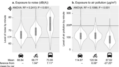
On average, per minute, motorists are exposed to sound levels of 66.84 dB(A), compared with 68.77 for cyclists, and 73.95 for public transit commuters (Table 3 and Fig. 5a). These differences are sig-nificant, and indicate that public transit users, and to a lesser extent cyclists, are more exposed to this nuisance, than those travelling by car. The higher levels observed for public transit commuters are explained in particular by their use of the subway. Moreover, for 5% of the duration of the public transit users' trips, the noise value even exceeded 80 dB(A) (P95 = 83.08;Table 3).
It should be noted that the World Health Organization (WHO) re-commends that the guideline value of 55 dB(A) should not be exceeded Fig. 3. Examples of regressions for predicting minute ventilation and MET.
Fig. 4. Route duration according to the mode of transportation. Table 2
Travel time differences from car users (in minutes).
Q1 Mean Median Q3 SD
Bicycle (N = 33) −5.07 0.77 0.32 5.87 12.92
Public transit (N = 33) −2.37 3.93 4.52 8.35 11.34 Q1:first quartile; Q3: third quartile; SD: standard deviation.
outdoors during the day. In addition, in its policy on road traffic noise, the Quebec Ministry of Transport, Sustainable Mobility and Transport Electrification recommends that noise not surpass 65 dB(A) along traffic lanes. These values are clearly being exceeded, whatever the mode of transport used.
As with noise, there are also significant differences in individual exposure to air pollution with the three modes of transportation: the levels of exposure to nitrogen dioxide (NO2) are on average 115, 121
and 88μg/m3 respectively for motorists, cyclists, and public transit
users (Table 3andFig. 5b). In other words, individual exposure to the pollutant is higher for cyclists compared with motorists and public transit commuters. Also, the levels of exposure are on average half the WHO short-term (1-h) NO2guideline value of 200μg/m3(World Health
Organization, 2006). Even the values for the 95th percentiles do not exceed this threshold (Table 3). Therefore, considering that the average duration of the trips is under 40 min, we can suppose that the levels of short-term exposure are not harmful to health, even for cyclists.
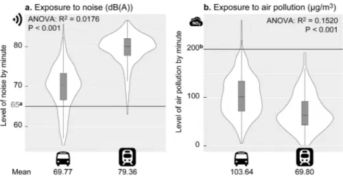
It is notable that the violin plots for noise exposure for public transit users show a bimodal distribution (Fig. 5a). We therefore hypothesize that the segments of the trips made by subway are noisier. To test this hypothesis, we separated the one-minute segments travelled in the subway from those travelled by bus and/or walking (walking from the origin or destination to the nearest station or bus stop). It is un-surprising that noise exposure is much higher in the subway (on average, 79 versus 70 dB(A) for the bus and/or walking), whereas air pollution exposure is lower (on average, 70 versus 104μg/m3) (Fig. 6).
3.3. Comparison of levels of nitrogen dioxide inhalation
Cyclists inhale, on average, nearly 3.69 times more of the pollutant than motorists (Table 4andFig. 7). This is of course explained by the higher levels of physical activity (4.12 times higher for cyclists than for car drivers) and thus much higher heart rates (1.58) and ventilation rates (3.52). In other words, they breathe more litres of air per minute into their lungs and therefore inhale more air and the pollutants it contains. For example, the median METs values are 1.52 (light-intensity activities), 7.64 (vigorous-intensity activities), and 3.77 (moderate-in-tensity activities) for motorists, cyclists, and public transit commuters respectively; the number of heart beats per minute are 72, 116 and 93; the median number of litres of air per minute is 13, 49 and 20; and the median number of micrograms of NO2inhaled per minute is 1.42, 5.65
and 1.66.
Using the data shown inTable 5, we can compare the total doses inhaled and the caloric expenditure over the entire trip for the three modes. Although there are no significant differences between the three modes of transportation for the duration of the trips (section 3.1), the inhaled doses are much greater for cyclists: on average, 193 micro-grams of NO2compared with 59 for motorists and 76 for public transit
users. And the caloric expenditure is of course also much higher for cyclists (367 cal on average), followed by public transit commuters (175 cal), and motorists (101 cal).
Table 3
Summary statistics for individual exposure to noise and air pollution per minute according to the mode of transportation.
Summary statistics Ratio from cara
P5 Q1 Mean Median Q3 P95 SD RA ARR
dB(A) Car 60.23 63.76 66.84 66.46 69.26 75.16 4.56 – – Bicycle 61.87 65.91 68.77 68.70 71.56 75.48 4.29 1.03 1.03 Public transit 61.20 69.48 73.95 74.58 79.77 83.08 6.79 1.11 1.10 NO2(μg/m3) Car 45.04 90.19 114.87 114.68 141.52 177.45 41.71 – – Bicycle 56.13 92.75 120.94 119.43 142.88 197.21 41.47 1.05 1.07 Public transit 24.49 55.96 87.62 82.72 117.37 161.90 43.37 0.75 0.70
P5: 5th percentile; Q1:first quartile; Q3: third quartile; P95: 95th percentile; SD: standard deviation.
a RA: ratio of averages; ARR: geometric average ratio of routes.
3.4. Comparison of the indicators in controlling for the effect of the participants and the devices: Results of the linear mixed-effects models
The linear mixed-effects models allow us to determine whether the differences observed with the ANOVAs are still significant after con-trolling for the effect of the participants (Table 6).
It should be noted that the impact of the participants (random ef-fects) is significant for the six models (see the Chi2values significant at
P = 0.000). Also, the ICC values indicate that a large proportion of the total variance of the heart rate and the ventilation rate is explained by the individual participants (23.7% and 28.9%), and, to a lesser degree, for the METs and NO2inhalation (7.3% and 7.8%). This is hardly
sur-prising as the age, weight, sex, and VO2max vary from participant to
participant. Another interesting point is that the total variance of the NO2measures is explained at a level of 11.5%. In other words, 11.5% of
the variance is explained by the NO2 sensor itself, which generally
corresponds to the precision of the sensor as reported by the Aeroqual company (< ± 10%). On the other hand, the impact of the dosimeter is much smaller (ICC = 3.7%).
Looking at the values of thefit statistics (AIC, BIC and pseudo R2),
the best-performing models are, in order, those with, as a dependent variable, ventilation, the METs, the heart rate, and the inhalation, with pseudo R2values greater than 0.5. On the other hand, the values for
individual exposure to NO2(0.166) and noise (0.262) are lower.
Once we have controlled for random effects (the participant), we can analyze thefixed effects, that is, the coefficients for the modes of transportation. Note that the value of the intercept corresponds to that for motorists. For example, for thefirst model, on average, noise ex-posure is 66.79 dB(A) for motorists, to which we can add 2.19 and 7.21 dB(A) for cyclists and public transit commuters respectively (that is, average exposures of 68.99 and 74.01 dB(A)). The regression coef-ficients obtained for cyclists and public transit commuters thus corre-spond to the differences from the mean by car shown inFigs. 5 and 7 and obtained using ANOVAs.
Compared with the ANOVAs, the results of the linear mixed-effects models are very similar (that is, the averages obtained are very similar). On the other hand, some differences are no longer significant when we consider individual variations. This is the case with NO2: although the
Fig. 6. Individual exposure to noise and air pollution by public transit (bus and subway).
Table 4
Summary statistics for pollutant inhalation and respiratory parameters per minute according to the mode of transportation.
Summary statistics Ratio from cara
P5 Q1 Mean Median Q3 P95 SD RA ARR
Heart rate (beats per minute)
Car 62.02 67.44 73.99 72.06 78.17 93.88 9.73 – –
Bicycle 90.46 104.83 116.59 116.28 128.33 142.99 16.23 1.58 1.57
Public transit 70.43 82.64 95.29 93.49 107.19 123.00 16.60 1.28 1.28
Ventilation (litres per minute)
Car 9.32 11.89 14.37 13.11 15.86 22.85 4.35 – –
Bicycle 28.97 40.16 50.55 48.58 60.31 77.16 14.85 3.52 3.50
Public transit 10.32 15.22 21.05 19.66 26.02 35.72 9.91 1.46 1.42
Metabolic equivalent of tasks (METs)
Car 0.80 1.20 1.84 1.52 2.07 4.16 1.03 – – Bicycle 4.79 6.69 7.59 7.64 8.75 10.12 1.61 4.12 4.54 Public transit 1.57 2.71 3.96 3.77 5.10 6.67 1.63 2.14 2.21 Inhalation (μg of NO2) Car 0.56 1.04 1.67 1.42 1.98 3.56 0.99 – – Bicycle 1.96 4.03 6.18 5.65 8.19 11.29 2.96 3.69 3.79 Public transit 0.36 0.89 1.93 1.66 2.71 4.45 1.29 1.15 1.02
P5: 5th percentile; Q1:first quartile; Q3: third quartile; P95: 95th percentile; SD: standard deviation.
averages differ among the three modes, these differences are no longer significant at a 5% threshold. However, for ventilation and inhalation, only the difference between motorists and public transit users is not significant, whereas it is significant between cyclists and motorists. 4. Discussion
4.1. Limitations of the study
One limitation of the study is that the trips by car were all made with the window open as in some earlier studies (De Nazelle et al., 2012; Dirks et al., 2012). During the collection period, the average temperatures were, respectively, 31, 27 and 29 °C for trips made by car, bike and public transit (measured using an Aeroqual temperature sensor). The levels of exposure to air pollution are generally lower in a car with the windows closed and the air conditioning on than with the window open (Cepeda et al., 2017). The same is obviously true for noise levels. Consequently, if the study had been performed with the car windows closed and the air conditioning on, three hypotheses can be
advanced regarding the results obtained. First, for noise exposure, the significant differences found between cyclists, public transit commuters and car users would have been even greater. Secondly, contrary to our findings, it is possible that the levels of exposure to NO2would have
been significantly lower for car users compared with the other two modes. In that case, this would mean that the ratio between the doses inhaled by cyclists and car users would also have been even higher. As done by other authors (Chertok et al., 2004; Quiros et al., 2013; Vouitsis et al., 2014), future research conducted in Montreal should ideally include both possible configurations for cars (window open versus windows closed with air conditioning on).
It is also appropriate to discuss the scope of the results for public transit which apply to large metropolises that have a subway system and not to medium-sized cities. For this mode of transport, we obtained much higher levels of exposure to noise, as well as much lower levels for air pollution, compared with travel by car and bicycle (respectively, 74, 67 and 69 dB(A), and 87, 115 and 121μg/m3for NO
2). However,
these large differences are mainly explained by the use of the noisier subway, which is also less polluted than the bus (79 dB(A) and 70μg/ Fig. 7. Individual physiological indicators and inhaled doses according to the mode of transportation.
m3versus 70 dB(A) and 104μg/m3). On the other hand, if we only compare the two modes of transport of bus and car, we may conclude that public transit is then slightly noisier than car travel (70 versus 67 dB(A)), but less polluted (114 versus 103μg/m3).
Afinal limitation that specifically concerns the case of Montreal is that the Montreal transportation agency is in the process of gradually implementing a newfleet of subway trains (AZUR subway trains) that are less noisy than the older model (MR-73) (85 dB(A) versus 90 dB(A) in the centre of the train) (BAPE, 2016).
4.2. Cycling: An effective rush-hour alternative to the car
Concerning travel times, using the car during rush-hour trips of about 10 km from peripheral neighbourhoods to downtown Montreal is not significantly faster than travelling by bike or public transit. In other words, cycling and public transit are effective alternatives to the car during rush hour. Indeed, cyclists arrive on average one minute after motorists, and public transit commuters, 4 min afterwards. Nor does this take into account the time required to park the car. The benefits of physical activity are obviously greater for cyclists: with a comparable duration and length of the trip (on average, 10 km and 38 min), they burn 3.63 times more calories than motorists. This ratio is also higher for public transit users (1.73) who combine several modes (walking, bus
torists are the most exposed in 30 cases out of a total of 42 comparisons, regardless of the pollutant selected. Moreover, out of 12 studies mea-suring pollutant inhalation, cyclists had the highest inhalation doses. It is not surprising that our results corroborate thefindings for inhalation, which is significantly higher for cyclists and public transit commuters compared with motorists. On the other hand, the results of the mixed-effects model show that there are no significant differences for exposure to nitrogen dioxide with the three modes.
4.4. Geography of the cycling network in Montreal
It is today well known that the type of road, bicycle path or lane and the proximity of the bicycle path to motor vehicle traffic lanes can have a significant impact on cyclists' exposure to air pollution and noise (Apparicio et al., 2016;Boogaard et al., 2009;Kingham et al., 2013; Knibbs and de Dear, 2010;Macnaughton et al., 2014).
Regarding the Island of Montreal, a recent study has shown that the cycling network has more than doubled in 25 years (from 1991 to 2016), increasing from 270 to 732 km, mainly in the central districts of the city (Houde et al., 2018). The same study also revealed that these districts usually chose to set up bike lanes and shared bike lanes due to their low cost (compared with off-street bicycle paths and on-street bike paths). Many of these bike lanes and shared bike lanes have thus been developed along major traffic arteries leading either north and south or east and west to the downtown area. Cyclists using these lanes are thus exposed to high concentrations of traffic-related pollutants and road traffic noise, especially during rush hours. Indeed, another Montreal study showed that noise and pollution levels are not significantly dif-ferent on bike lanes and shared bike lanes compared with collector
Public transit (N = 18)
171.20 175.07 190.44 209.16 49.35 1.73 1.78
Q1:first quartile; Q3: third quartile; SD: standard deviation.
a RA: ratio of averages; ARR: geometric average ratio of routes.
Table 6
Results of the linear mixed-effects models.
Dependent variable dB(A) NO2(μg/m3) Heart rate Minute ventilation Metabolic equivalent of tasks Inhalation (μg of NO2)
Fixed effects (estimate and t values)
Intercept 66.79*** (107.82) 114.82*** (10.90) 73.99*** (13.70) 14.38*** (3.55) 1.85*** (6.41) 1.68*** (4.35)
Bicycle 2.19** (2.50) 6.37 (0.43) 42.34*** (5.54) 35.97*** (6.28) 5.74*** (14.07) 4.49*** (8.22)
Public transit 7.21*** (8.24) −27.10 (−1.82) 21.31** (2.79) 6.67 (1.16) 2.11** (2.98) 0.25 (0.46)
Variance partitioning (random effects)
Between participants 1.07 217.3 57.74 32.59 0.1593 0.2866
Residual 28.17 1672.6 186.26 80.19 2.0308 3.3986
Intra-class correlation (ICC) 3.67 11.49 23.66 28.90 7.27 7.78
Chi2 71.2 128.0 232 303 62.2 61.5 P 0.000 0.000 0.000 0.000 0.000 0.000 Fit statistics Number of observations 3425 2142 1901 1901 1901 1901 LogLik −10,586 −10,989 −7670 −6871 −3380 −3869 AIC 21,182 21,987 15,350 13,752 6770 7748 BIC 21,213 22,016 15,378 13,780 6798 7775 Pseudo R2 0.262 0.166 0.625 0.754 0.725 0.549 T values in parentheses. Signif. codes:‘***’ 0.001 ‘**’ 0.01 ‘*’ 0.05.
streets, although they are much lower on on-street bicycle paths and off-street bicycle paths (Apparicio et al., 2016). This may explain why we found comparable levels of exposure to air pollution between cy-clists and car users, and higher noise levels for cycy-clists. This then raises major urban planning issues.
4.5. Measuring cyclists' exposure: a planning issue
Urban planners today consider cycling as a means of transportation that helps to reduce greenhouse gases and road congestion. For ex-ample, in the Montreal Metropolitan Community's most recent urban development plan, cycling is seen as an integrated planning component in urban planning and transportation, which represents a mini-revolu-tion in a historically car-oriented metropolis. Moreover, the City of Montreal plans to invest $225 million over the next 15 years to extend its cycling network and encourage the practice of bicycling.
Our results show that cyclists inhale far more nitrogen dioxide (NO2) than motorists (3.7 times more) and are slightly more exposed to
noise (2.19 dB(A)). Such disparities, to cyclists' detriment, can be con-sidered as a form of environmental inequity (Walker, 2009, 2012); they are much more exposed to pollutants that they do not generate.
To decrease these inequities, if we consider cycling as a means of reducing road congestion and greenhouse gases, new cycling infra-structures connected with the downtown area should be planned along routes where the levels of noise and pollution are lower. To achieve this, measures of the concentration of or exposure to air pollution and road traffic noise should be included when choosing the location of new cycling infrastructures. Another option is to develop cycling super-highways facilitating commuting, while ensuring that these routes are for cyclists only, in order to limit their exposure to noise and air pol-lutants. This would help to increase the flow of cycling traffic and heighten cyclists' sense of security, while lowering the risk of accidents. And such superhighways would undoubtedly encourage many people to bicycle to work and thus reduce the modal share of cars in rush-hour commuting, as well as greenhouse gases. Although the construction of these cycling infrastructures is expensive, the implementation of an urban transport policy promoting active mobility remains very bene-ficial collectively. For example,Macmillan et al. (2014)emphasize that every dollar invested in cycling infrastructures results in a ten times greater savings in public health services, especially in reducing mor-bidity and mortality associated with physical inactivity and air pollu-tion.
5. Conclusion
During rush hours in Montreal (8 am and 5 pm), the comparison of trips of about 10 km made using three varied modes of transportation enabled us to show that travel times do not significantly differ among cyclists, motorists, and public transit commuters. The use of mixed models demonstrated that public transit commuters' and cyclists' levels of exposure to noise are significantly greater than motorists' exposure. Again, using mixed models, we found that although the levels of ex-posure to the NO2pollutant do not significantly differ among the three
modes, the inhaled doses of NO2pollutant are more than three times
higher for cyclists than for motorists due to their stronger ventilation rate. It is no surprise that the levels of physical activity and caloric expenditure, as well as the health benefits, are far greater for cyclists than for motorists.
Several avenues are worth exploring in future studies. It would also be pertinent to examine the associations between exposure to these two nuisances (noise and air pollution), ventilation, pollutant inhalation, and the urban form of the city. To accomplish this, the data should be collected by using the same measuring devices and the same metho-dology in various other big cities around the world. The choice of these cities should include cities in both the North and South that present differing levels of air and noise pollution. Developing a database
assembled from data collected in a number of cities would also make it possible to more finely explore the relations between the urban en-vironment and cyclists' levels of exposure.
Acknowledgments
The authors would like to thank the students of INRS Urbanisation Culture Société involved in this research for their time and cooperation, and the three anonymous reviewers for their careful reading of our manuscript and their many insightful comments and suggestions. The authors are also grateful for the financial support provided by the Canada Research Chair in Environmental Equity (950-230813).
References
Allan, M., Richardson, G.M., 1998. Probability density functions describing 24-hour in-halation rates for use in human health risk assessments. Hum. Ecol. Risk. Assess. 4, 379–408.
Apparicio, P., Carrier, M., Gelb, J., Séguin, A.-M., Kingham, S., 2016. Cyclists' exposure to air pollution and road traffic noise in central city neighbourhoods of Montreal. J. Transp. Geogr. 57, 63–69.
BAPE, 2016. Rapport 331. Projet de Réseau Électrique Métropolitain de Transport Collectif. Bureau d'audiences publiques sur l'environnement, Montreal, pp. 296. Bates, D., Mächler, M., Bolker, B., Walker, S., 2015. Fitting linear mixed-effects models
using lme4. J. Stat. Softw. 67, 1–48.
Boogaard, H., Borgman, F., Kamminga, J., Hoek, G., 2009. Exposure to ultrafine and fine particles and noise during cycling and driving in 11 Dutch cities. Atmos. Environ. 43, 4234–4242.
Briggs, D.J., de Hoogh, K., Morris, C., Gulliver, J., 2008. Effects of travel mode on ex-posures to particulate air pollution. Environ. Int. 34, 12–22.
Cepeda, M., Schoufour, J., Freak-Poli, R., Koolhaas, C.M., Dhana, K., Bramer, W.M., Franco, O.H., 2017. Levels of ambient air pollution according to mode of transport: a systematic review. Lancet Public Health 2, e23–e34.
Chertok, M., Voukelatos, A., Sheppeard, V., Rissel, C., 2004. Comparison of air pollution exposure forfive commuting modes in Sydney-car, train, bus, bicycle and walking. Health Promot. J. Australia 15, 63–67.
Core Team, R., 2017. R: A Language and Environment for Statistical Computing. R Foundation for Statistical Computing, Vienna, Austria. https://www.R-project.org/. Ville de Montréal, 2017. Montréal, Ville Cyclable. Plan-Cadre Vélo: Sécurité, Efficience,
Audace. pp. 31.
De Nazelle, A., Fruin, S., Westerdahl, D., Martinez, D., Ripoll, A., Kubesch, N., Nieuwenhuijsen, M., 2012. A travel mode comparison of commuters' exposures to air pollutants in Barcelona. Atmos. Environ. 59, 151–159.
Dirks, K.N., Sharma, P., Salmond, J.A., Costello, S.B., 2012. Personal exposure to air pollution for various modes of transport in Auckland, New Zealand. Open Atmos. Sci. J. 6.
Dons, E., Panis, L.I., Van Poppel, M., Theunis, J., Wets, G., 2012. Personal exposure to black carbon in transport microenvironments. Atmos. Environ. 55, 392–398. Dons, E., Laeremans, M., Orjuela, J.P., Avila-Palencia, I., Carrasco-Turigas, G.r.,
Cole-Hunter, T., Anaya-Boig, E., Standaert, A., De Boever, P., Nawrot, T., 2017. Wearable sensors for personal monitoring and estimation of inhaled traffic-related air pollution: evaluation of methods. Environ. Sci. Technol. 51, 1859–1867.
Duci, A., Chaloulakou, A., Spyrellis, N., 2003. Exposure to carbon monoxide in the Athens urban area during commuting. Sci. Total Environ. 309, 47–58.
Goel, R., Gani, S., Guttikunda, S.K., Wilson, D., Tiwari, G., 2015. On-road PM 2.5 pol-lution exposure in multiple transport microenvironments in Delhi. Atmos. Environ. 123, 129–138.
Hill, L.B., Gooch, J., 2007. A multi-city investigation of exposure to diesel exhaust in multiple commuting modes. Clean Air Task Force Spec. Rep. 1.
Houde, M., Apparicio, P., Séguin, A.-M., 2018. A ride for whom: has cycling network expansion reduced inequities in accessibility in Montreal, Canada? J. Transp. Geogr. 68, 9–21.
Huang, J., Deng, F., Wu, S., Guo, X., 2012. Comparisons of personal exposure to PM 2.5 and CO by different commuting modes in Beijing, China. Sci. Total Environ. 425, 52–59.
Kaur, S., Nieuwenhuijsen, M., Colvile, R., 2005. Personal exposure of street canyon in-tersection users to PM 2.5, ultrafine particle counts and carbon monoxide in Central London, UK. Atmos. Environ. 39, 3629–3641.
Kim, M., Chang, S.I., Seong, J.C., Holt, J.B., Park, T.H., Ko, J.H., Croft, J.B., 2012. Road traffic noise: annoyance, sleep disturbance, and public health implications. Am. J. Prev. Med. 43, 353–360.
Kingham, S., Longley, I., Salmond, J., Pattinson, W., Shrestha, K., 2013. Variations in exposure to traffic pollution while travelling by different modes in a low density, less congested city. Environ. Pollut. 181, 211–218.
Knibbs, L.D., de Dear, R.J., 2010. Exposure to ultrafine particles and PM 2.5 in four Sydney transport modes. Atmos. Environ. 44, 3224–3227.
Laumbach, R., Meng, Q., Kipen, H., 2015. What can individuals do to reduce personal health risks from air pollution? J. Thoracic dis. 7, 96.
Lewne, M., Nise, G., Lind, M.-L., Gustavsson, P., 2006. Exposure to particles and nitrogen dioxide among taxi, bus and lorry drivers. Int. Arch. Occup. Environ. Health 79, 220–226.
Suárez, L., Mesías, S., Iglesias, V., Silva, C., Cáceres, D.D., Ruiz-Rudolph, P., 2014. Personal exposure to particulate matter in commuters using different transport modes (bus, bicycle, car and subway) in an assigned route in downtown Santiago, Chile. Environ. Sci. 16, 1309–1317.
U.S. EPA, 2011. Chapter 6—Inhalation Rates, Exposure Factors Handbook: 2011 Edition.
Zuurbier, M., Hoek, G., Oldenwening, M., Lenters, V., Meliefste, K., van den Hazel, P., Brunekreef, B., 2010. Commuters' exposure to particulate matter air pollution is af-fected by mode of transport, fuel type, and route. Environ. Health Perspect. 118, 783–789.