Université de Montréal
Analyse bayésienne et classification pour modèles continus modifiés à zéro
par
Félix Labrecque-Synnott
Département de mathématiques et de statistique Faculté des arts et des sciences
Thèse présentée à la Faculté des études supérieures en vue de l’obtention du grade de Philosophiæ Doctor (Ph.D.)
en statistique
16 août, 2010
c
Faculté des études supérieures
Cette thèse intitulée:
Analyse bayésienne et classification pour modèles continus modifiés à zéro
présentée par: Félix Labrecque-Synnott
a été évaluée par un jury composé des personnes suivantes: Alejandro Murua, président-rapporteur
Jean-François Angers, directeur de recherche Mylène Bédard, membre du jury Jean-Philippe Boucher, examinateur externe
William J. McCausland, représentant du doyen de la FES
RÉSUMÉ
Les modèles à sur-représentation de zéros discrets et continus ont une large gamme d’applications et leurs propriétés sont bien connues. Bien qu’il existe des travaux portant sur les modèles discrets à sous-représentation de zéro et modifiés à zéro, la formulation usuelle des modèles continus à sur-représentation – un mélange entre une densité continue et une masse de Dirac – empêche de les généraliser afin de couvrir le cas de la sous-représentation de zéros. Une formulation alternative des modèles continus à sur-représentation de zéros, pouvant aisément être généralisée au cas de la sous-représentation, est présentée ici. L’estimation est d’abord abordée sous le paradigme classique, et plusieurs méthodes d’obtention des estimateurs du maximum de vraisemblance sont proposées. Le problème de l’estimation ponctuelle est également considéré du point de vue bayésien. Des tests d’hypothèses classiques et bayésiens visant à déterminer si des données sont à sur- ou sous-représentation de zéros sont présentées. Les méthodes d’estimation et de tests sont aussi évaluées au moyen d’études de simulation et appliquées à des données de précipitation agrégées. Les diverses méthodes s’accordent sur la sous-représentation de zéros des données, démontrant la pertinence du modèle proposé.
Nous considérons ensuite la classification d’échantillons de données à sous-représentation de zéros. De telles données étant fortement non normales, il est pos-sible de croire que les méthodes courantes de détermination du nombre de grappes s’avèrent peu performantes. Nous affirmons que la classification bayésienne, basée sur la distribution marginale des observations, tiendrait compte des particularités du modèle, ce qui se traduirait par une meilleure performance. Plusieurs méthodes de classification sont comparées au moyen d’une étude de simulation, et la mé-thode proposée est appliquée à des données de précipitation agrégées provenant de 28 stations de mesure en Colombie-Britannique.
Mots clés : sous-représentation de zéros, déflation à zéro, méthode d’agrégation bayésienne, précipitations agrégées, distribution de Laplace tronquée, algorithme EM, modèles de mélanges.
Zero-inflated models, both discrete and continuous, have a large variety of ap-plications and fairly well-known properties. Some work has been done on zero-deflated and zero-modified discrete models. The usual formulation of continuous zero-inflated models – a mixture between a continuous density and a Dirac mass at zero – precludes their extension to cover the zero-deflated case. We introduce an alternative formulation of zero-inflated continuous models, along with a natural extension to the zero-deflated case. Parameter estimation is first studied within the classical frequentist framework. Several methods for obtaining the maximum likelihood estimators are proposed. The problem of point estimation is considered from a Bayesian point of view. Hypothesis testing, aiming at determining whether data are zero-inflated, zero-deflated or not zero-modified, is also considered under both the classical and Bayesian paradigms. The proposed estimation and testing methods are assessed through simulation studies and applied to aggregated rainfall data. The data is shown to be zero-deflated, demonstrating the relevance of the proposed model.
We next consider the clustering of samples of zero-deflated data. Such data present strong non-normality. Therefore, the usual methods for determining the number of clusters are expected to perform poorly. We argue that Bayesian cluster-ing based on the marginal distribution of the observations would take into account the particularities of the model and exhibit better performance. Several clustering methods are compared using a simulation study. The proposed method is applied to aggregated rainfall data sampled from 28 measuring stations in British Columbia.
Keywords: zero-deflation, aggregate rainfall, truncated Laplace, Bayesian aggregation, EM algorithm, mixture models
TABLE DES MATIÈRES
RÉSUMÉ . . . . iii
ABSTRACT . . . . iv
TABLE DES MATIÈRES . . . . v
LISTE DES TABLEAUX . . . viii
LISTE DES FIGURES . . . . ix
LISTE DES SIGLES . . . . x
NOTATION . . . . xi DÉDICACE . . . xii REMERCIEMENTS . . . xiii INTRODUCTION . . . . 1 Références . . . 6 RÉFÉRENCES . . . . 7
CHAPTER 1: AN EXTENSION OF ZERO-MODIFIED MODELS TO THE CONTINUOUS CASE . . . 10
ABSTRACT . . . 12 1.1 Introduction . . . 12 1.2 The model . . . 15 1.3 Estimation . . . 17 1.4 Asymptotic properties . . . 22 1.5 Simulation results . . . 25
1.6 Application to real data . . . 31
1.7 Concluding remarks . . . 35
References . . . 36
REFERENCES . . . 37
CHAPTER 2: BAYESIAN ESTIMATION AND TESTING FOR CONTI-NUOUS ZERO-MODIFIED MODELS . . . 41
ABSTRACT . . . 43 2.1 Introduction . . . 43 2.2 The model . . . 44 2.3 Estimation . . . 47 2.4 Numerical methods . . . 48 2.4.1 Adaptive Monte-Carlo . . . 48
2.4.2 Adaptive Gaussian quadrature . . . 49
2.4.3 Gauss-Legendre-Laguerre quadrature . . . 51
2.5 Hypothesis testing . . . 52
2.6 Simulation and application results . . . 52
2.7 Concluding remarks . . . 57
References . . . 59
REFERENCES . . . 60
CHAPTER 3: BAYESIAN MODEL-BASED CLUSTERING OF CONTI-NUOUS ZERO-MODIFIED DATA . . . 62
ABSTRACT . . . 63
3.1 Introduction . . . 63
3.2 The model . . . 64
3.3 Contiguous model-based clustering . . . 66
vii
3.4.1 Je(2)/Je(1) . . . 70
3.4.2 Beale test . . . 70
3.4.3 pseudo-F . . . 71
3.4.4 AIC . . . 72
3.5 Application to a real dataset . . . 76
3.6 Concluding remarks . . . 80 References . . . 80 REFERENCES . . . 81 CHAPITRE 4 : CONCLUSION . . . 83 4.1 Travaux futurs . . . 86 Références . . . 88 RÉFÉRENCES . . . 89
1.1 Simulation results for (p, x0, τ, µ, λ) = (−.1, 1, .5, 1, 2) . . . 30
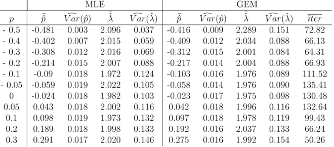
1.2 Simulation results as p varies, with µ = 0, x0 = 1, τ = 0.5, and
λ= 2 . . . 31 1.3 Simulation results for ˆpmle when f0 ∝ f1, (x0, µ, λ) = (0.5, 1, 1) 32
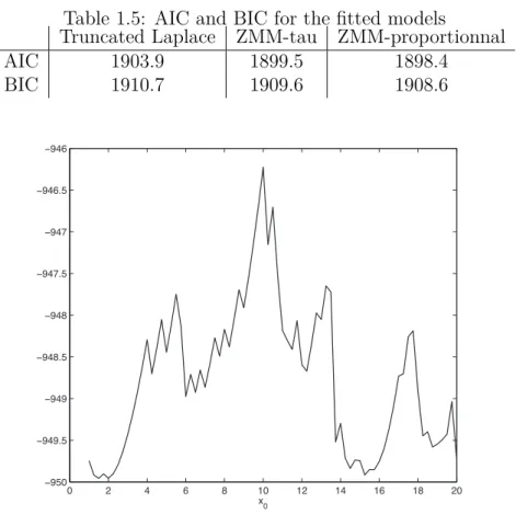
1.4 MLEs and standard errors for the fitted models . . . 32 1.5 AIC and BIC for the fitted models . . . 34 2.1 Mean and variance of parameter estimates as a function of n,
with p = −0.1, µ = λ = 20 . . . 54 2.2 Mean and variance of parameter estimates as a function of p,
µ= λ = 20, n = 50 . . . . 54 2.3 Power as a function of n, with p = −0.1, µ = λ = 20 . . . 58 2.4 Power as a function of p, µ = λ = 20, n = 50 . . . . 58 2.5 Estimation of a real data set of aggregated rainfall data . . . . 58 2.6 Testing a real data set of aggregated rainfall data . . . 58 3.1 Probability of identifying the correct clusters . . . 74 3.2 Average number of misclassified sites . . . 74 3.3 Measuring stations and their MLE, (x0, τ) = (10, 0.05) . . . . 78
LISTE DES FIGURES
1.1 Bound pmin as a function of µ, λ fixed . . . . 27
1.2 Bound pmin as a function of λ, µ fixed . . . . 27
1.3 f1 and f for (p, τ, µ, λ) = (−0.1, 1/2, 1, 2) . . . 29
1.4 Densities f and f1 for f0 ∝ f1, p = −.05 and p = .05 . . . 33
1.5 Data and fitted models for Montreal precipitations . . . 33
1.6 Log-likelihood as a function of x0 and τ for f0 ∝ (x0− x)τ . . 33
1.7 Log-likelihood as a function of x0 for f0(x) ∝ f1(x|θ)I[0,x0](x) . 34 2.1 Posterior probabilities for tests as a function of n. . . . 56
3.1 The two probability density functions used in scenario 2 . . . 74
3.2 Prince Rupert data, fitted ZMM and fitted truncated Laplace 77 3.3 Measuring stations and clusters for British Columbia . . . 79
cdf fonction de répartition (cumulative distribution function) EMV estimateur du maximum de vraisemblance
MAP maximum a posteriori
MLE estimateur du maximum de vraisemblance (maximum likelihood estimator) MMZ modèle modifié à zéro (zero-modified model)
pmf fonction de masse (probability mass function) pdf fonction de densité (probability density function) ZDM modèle dégonflé à zéro (zero-deflated model)
ZIM modèle gonflé à zéro (zero-inflated model) ZMM modèle modifié à zéro (zero-modified model)
NOTATION
f1(x|θ) la fonction de densité de base
f0(x) la fonction de densité de modification
R+ les nombres réels non négatifs
nsamples le nombre d’échantillons considérés en classification
θ les paramètres de la densité de base
Θ l’espace paramétrique de la densité de base ω les paramètres d’intérêt (θ, p)
Ω l’espace paramétrique sous le MMZ |A| la cardinalité de l’ensemble A.
REMERCIEMENTS
J’aimerais tout d’abord remercier mon directeur de thèse, Jean-François Angers, pour son soutient et ses conseils tout au long de mes études doctorales.
Je remercie également Yves Lepage, m’ayant donné une première appréciation de la théorie statistique, et dont le cours me convainquit finalement d’opter pour cette spécialisation au baccalauréat, pour ensuite continuer aux cycles supérieurs. Je voudrais également souligner l’excellent travail du personnel administratif du département. Merci également à mes parents et ma soeur Delphine pour leurs appuis et encouragements au long de ces quatre années, ainsi qu’à Éloïse et André. Merci au FQRNT, au CRSNG, au Département de mathématiques et de sta-tistique et à la Faculté des études supérieures et postdoctorales pour les bourses m’ayant été octroyées lors de mes études doctorales. Je souhaite aussi remercier Jean-François et Véronique Hussin pour m’avoir donné l’opportunité d’une pre-mière expérience d’enseignement universitaire, et André Montpetit pour ses conseils relatifs à l’utilisation de LATEX et pour m’avoir donné une belle expérience de travail
Nous traitons ici de modèles continus modifiés à zéro, utilisés lorsque la pro-portion de zéros dans les observations diffère de ce qui serait prévu par un certain modèle.. La plupart des modèles modifiés à zéro rencontrés dans la littérature sont des modèles discrets : en effet, les modèles continus comportent certaines particu-larités rendant moins aisée l’utilisation de modèles modifiés à zéro. En particulier, la formulation usuelle des modèles continus gonflés à zéro ne permet pas de traiter également le cas d’un plus faible taux de zéros dans les observations. Nous pro-posons une nouvelle formulation, sous laquelle un modèle de base sera modifié sur un intervalle autour de zéro. À la limite, lorsque la taille de l’intervalle approche de zéro, la formulation classique des modèles continus gonflés à zéro est retrouvée. La nouvelle formulation permet le traitement de la sous-représentation de zéros, et sert également à la modélisation lorsque a proportion d’observations dans un intervalle autour de zéro diffère de la proportion prévue par un modèle donné. Cette formulation proposée est donc plus générale que la formulation classique des modèles continus gonflés à zéro.
Le développement de ce modèle est motivé par l’analyse de précipitations. La proportion de zéros dans ces données varie énormément selon le pas de temps consi-déré (des données journalières ayant une forte proportion de zéros, et des données mensuelles en ayant très peu). Ce problème de la proportion de zéros dans les don-nées de précipitation est complexifié par le fait que de très faibles précipitations peuvent ne pas être détectées par les pluviomètres, ou n’être enregistrées que comme « traces » de précipitations. La documentation d’Environnement Canada (http:// www.climate.weatheroffice.gc.ca/prods\_servs/index\_e.html\#cdcd) men-tionne qu’une valeur de 0 mm de précipitation peut correspondre à une absence de précipitations (le cas le plus fréquent), mais aussi à des traces de précipitations, des précipitations de quantité incertaine ou encore à une possibilité de précipitation (sans qu’il soit possible de trancher dans un sens ou dans l’autre). Des données de ce type sont analysées afin d’illustrer la classe de modèles proposée.
2 Cette thèse traite de modèles continus modifiés à zéro (MMZ, en anglais zero-modified models, ou ZMM ). La classe des MMZ comprend les modèles à sur-représentation de zéros (ou modèles gonflés à zéro, en anglais zero-inflated models ou ZIM ) et les modèles à sous-représentation de zéros (ou dégonflés à zéro, en an-glais zero-deflated models ou ZDM ), correspondant respectivement à une plus forte et une plus faible proportion de zéros dans les données que ce que nous donnerait un modèle de base.
Considérons d’abord le cas discret, plus fréquemment traité dans la littérature. Si X dénote une variable aléatoire distribuée d’après un modèle (discret) modifié à zéro, alors elle sera de fonction de masse
fX(x|p) = p+ (1 − p)f1(0|θ) au point x = 0 (1 − p)f1(x|θ) partout ailleurs, (1)
où f1(x|θ) dénote la fonction de masse de base, dépendant d’un paramètre θ
ha-bituellement inconnu. Puisque p sera généralement aussi un paramètre inconnu, nous dénotons, tout au long de cette thèse et tant pour le cas discret que continu, l’ensemble des paramètres d’intérêt (p, θ) par ω. Similairement, alors que Θ repré-sente l’espace paramétrique associé au modèle de base f1,nous dénotons Ω l’espace
paramétrique du modèle modifié à zéro (le produit cartésien de Θ et de l’ensemble des valeurs possibles pour p).
Si p est positif, et ce tant pour le cas discret que continu, l’équation (1) est un mélange entre une masse de Dirac au point 0 et la fonction de masse de base. Ce paramètre peut aussi être vu comme une quantité ajoutée à la probabilité que X soit identiquement égale à zéro. Fréquent dans la littérature scientifique, ce type de modèle fut d’abord présenté dans Singh (1963). Il s’agissait alors d’une loi de Pois-son avec sur-représentation de zéros. L’estimation par maximum de vraisemblance (EMV) et ses propriétés asymptotiques pour ce modèle sont présentées dans El-Shaarawi (1985). De là, l’usage de ces modèles s’est répandu, et des modèles plus complexes furent construits sur cette première fondation (Lambert, 1992, Hall,
2000, Ridout et al., 2001, Dalrymple et al., 2003, Ghosh et al., 2006, Rodrigues, 2003, Van den Broek, 1995, Jansakul et Hinde, 2002, Gupta et al., 2005, Hasan et Sneddon, 2009).
La fonction de masse (1) demeure valide si p prend des valeurs négatives, mais supérieures à −f1(0|θ)/[1 − f1(0|θ)], f1(0|θ) 6= 1. La littérature scientifique est très
peu abondante à ce sujet ; en fait, bien que certain articles traitant de modèles discrets modifiés à zéros mentionnent le cas de la sous-représentation en plus de celui de la sur-représentation, aucun n’y est entièrement dédié. Des distributions de Poisson modifiées à zéro sont toutefois abordées dans Angers et Biswas (2003) et Dietz et Böhning (2000). Il faut noter qu’il ne s’agit plus d’un modèle de mélanges, et il est uniquement possible d’interpréter p comme une quantité retranchée à la probabilité que X prenne la valeur 0.
Dans le cas de modèles continus (f1(x|θ) est alors une fonction de densité), seul
le cas de la sur-représentation de zéros est mentionné dans la littérature. L’ap-proche utilisée dans ce cas est de prendre comme distribution pour X une masse de Dirac au point 0 avec probabilité p et la densité de base f1(x|θ) avec
pro-babilité (1 − p). Le modèle (1) n’est alors plus continu, mais mixte. Il est aussi possible d’interpréter p comme la probabilité que X soit identiquement égale à 0. Bien que moins fréquemment rencontrés dans la littérature que les modèles dis-crets gonflés à zéro, les modèles continus gonflés à zéro, présentées dans Aitchison (1955), ont toutefois diverses applications, principalement en sciences biologiques (Lo et al., 1992, Stefansson, 1996) et en modélisation de précipitations (Fernandes et al., 2009, Feuerverger, 1979). Notons qu’aucune des deux interprétations pos-sibles pour p dans ce cas ne permet de considérer des valeurs négatives pour ce paramètre.
Le but premier de cette thèse est de développer une formulation alternative pour les modèles continus gonflés à zéro pouvant aussi s’adapter au cas de la sous-représentation. La formulation proposée, à la limite, devient équivalente à la formulation usuelle. Les modèles continus modifiés à zéro constituent donc le lien unissant ces trois articles. Le premier article, après un relevé de la littérature
4 existante au sujet des modèles discrets à sur- et sous-représentation de zéros et des modèles continus à sur-représentation de zéros, présente le nouveau modèle proposé. Celui-ci est continu et permet de traiter le cas de la sous-représentation de zéros. L’estimation par maximum de vraisemblance y est aussi abordée. Le second article en constitue la prolongation directe, traitant d’estimation ponctuelle bayésienne et de tests d’hypothèses permettant de tester pour la sur- (p > 0), sous- (p < 0) représentation de zéros, ou encore la non modification (p = 0). Le troisième article est centré sur une application plus complexe de cette classe de modèles. Il s’agit de la création de régions homogènes à partir de données continues modifiées à zéro, c’est-à-dire de la classification d’échantillons de tels données, sous une contrainte de contiguïté. En effet, nous souhaitons que les régions ainsi soient contigües (c’est-à-dire non disjointes). Ce dernier article explore donc différents critères d’arrêt pour la classification hiérarchique agglomérative dans ce contexte. La classe des modèles continus modifiés à zéro constitue donc le principal fil conducteur de la thèse, les deux premiers articles la développant et en explorant l’estimation, alors que le troisième article en présente une application plus complexe.
Les applications considérées sont le second fil conducteur de la thèse. Le dé-veloppement de la classe des modèles continus modifiés à zéro fut principalement motivé par certains types de données – les précipitations agrégées sur 7, 14 ou 30 jours – et les deux premiers articles présentent une application des méthodes d’esti-mation proposées à un tel jeu de données. Cette application motive aussi en partie le choix de la densité de base f1(x|θ) proposée dans les trois articles, et utilisée lors
des applications présentées : les observations sont continues, positives, comportent des zéros, et semblent être dégonflées à zéro. De telles applications nécessitent donc une distribution continue, définie sur les réels positifs, et dont la fonction de densité n’est pas nulle au point 0, ce qui exclut potentiellement les distributions gamma et lognormale. La distribution de Laplace (ou double exponentielle) tronquée sur les réels positifs satisfait à ces critères.
Les deux premiers articles se terminent par l’application des méthodes d’es-timation ponctuelles à un jeu de données de précipitations montréalaises
bimen-suelles. Outre la cohérence entre les résultats donnés par les différentes méthodes lorsqu’appliquées à ces données, soulignons que l’utilisation de critères d’informa-tion (critère d’informad’informa-tion d’Akaike (Akaike, 1974), critère d’informad’informa-tion bayésien (Schwarz, 1978), tous deux fréquemment utilisés en sélection de modèles (Kuha, 2004, Yang, 2005, Burnham et Anderson, 2004)) et de tests d’hypothèses (test du rapport de vraisemblance, test de score, et les tests bayésiens présentés au second article) permet de conclure que ces données sont bel et bien modifiées à zéro. Nous entendons par là que l’augmentation de la vraisemblance lorsque nous passons du modèle de base (Laplace tronquée sur les réels positifs) au modèle modifié à zéro est assez grande pour justifier la plus grande complexité du modèle (telle que définie par l’AIC et le BIC). En outre, l’hypothèse p = 0, correspondant à un modèle non modifié à zéro, est rejetée indépendamment du test considéré.
Les deux premiers articles ayant confirmé la pertinence de la classe de mo-dèles proposée et son applicabilité à la modélisation de données de précipitations agrégées, le troisième propose de s’attaquer à un problème plus complexe (la clas-sification d’échantillons de données continues modifiées à zéro). Nous considérons plusieurs échantillons, correspondant à des point géographiques donnés, et nous nous intéressons à la classification de ces échantillons en grappes homogènes et contigües (ne contenant pas de sites géographiquement disjoints). Dans ce contexte, nous privilégions l’utilisation de méthodes de classification hiérarchiques agglomé-ratives. Si nous avons des mesures provenant de nsamples sites, nous considérerons
d’abord chacun de ces nsamples échantillons comme appartenant à une grappe
diffé-rente. Les méthodes de classification hiérarchiques nécessitent alors, itérativement, de construire une matrice de distance (ou de dissimilarité) entre les grappes et de tester si les deux grappes les moins distantes peuvent être combinées. Il faut noter ici que la matrice de distance ne fait pas référence à la distance géographique mais bien à une façon donnée de calculer des distances entre groupes d’observations. Par exemple, on pourrait prendre pour distance entre deux grappes la distance euclidienne entre les moyennes des observations comprises dans ces grappes. Cette approche est privilégiée dans ce contexte, puisqu’il sera plus intuitif de vérifier que
6 les grappes à combiner sont bel et bien adjacentes (classification hiérarchique ag-glomérative) que de vérifier que le partitionnement d’une grappe en deux ne crée pas de « trous » dans l’une des deux grappes résultantes (classification hiérarchique divisive).
Cette problématique est motivée par l’analyse de données de précipitations agrégées sur un territoire géographique donné (plutôt qu’en un seul point donné, comme c’était le cas dans l’application présentée dans les deux premiers articles). Les précipitations agrégées sur une base hebdomadaire, bimensuelle ou mensuelle étant utilisées en planification agronome (Azhar et al., 1992, Sharda et Das, 2005), en prévision d’écoulement des rivières (Dibike et Solomatine, 2001), en gestion de bassin-versants (Raghuwanshi et al., 2006) et en estimation d’abondance d’es-pèces (Eklundh, 1998, Peco et al., 1998), la classification de différents sites sur un territoire donné en régions homogènes en termes de précipitations agrégées serait d’intérêt pour plusieurs domaines d’application. Plusieurs stations de mesures en Colombie-Britannique sont considérées, ce territoire étant choisi pour ses précipi-tations abondantes et son relief intéressant.
Aitchison, J. (1955). On the distribution of a positive random variable having a discrete probability mass at the origin. Journal of the American Statistical Association, 50(271):901–908.
Akaike, H. (1974). A new look at the statistical model identification. IEEE tran-sactions on automatic control, 19(6):716–723.
Angers, J. et Biswas, A. (2003). A Bayesian analysis of zero-inflated generalized Poisson model. Computational statistics & data analysis, 42(1-2):37–46.
Azhar, A., Murty, V. et Phien, H. (1992). Modeling irrigation schedules for lowland rice with stochastic rainfall. Journal of Irrigation and Drainage Engineering, 118:36.
Burnham, K. et Anderson, D. (2004). Multimodel inference : understanding AIC and BIC in model selection. Sociological Methods & Research, 33(2):261.
Dalrymple, M. L., Hudson, I. L. et Ford, R. P. K. (2003). Finite mixture, zero-inflated Poisson and hurdle models with application to SIDS. Computational Statistics & Data Analysis, 41(3-4):491–504.
Dibike, Y. et Solomatine, D. (2001). River flow forecasting using artificial neural networks. Physics and Chemistry of the Earth, Part B : Hydrology, Oceans and Atmosphere, 26(1):1–7.
Dietz, E. et Böhning, D. (2000). On estimation of the Poisson parameter in zero-modified Poisson models. Computational statistics & data analysis, 34(4):441– 459.
Eklundh, L. (1998). Estimating relations between AVHRR NDVI and rainfall in East Africa at 10-day and monthly time scales. International Journal of Remote Sensing, 19(3):563–570.
8 El-Shaarawi, A. (1985). Some goodness-of-fit methods for the Poisson plus added
zeros distribution. Applied and environmental microbiology, 49(5):1304.
Fernandes, M., Schmidt, A. et Migon, H. (2009). Modelling zero-inflated spatio-temporal processes. Statistical Modelling, 9(1):3.
Feuerverger, A. (1979). On some methods of analysis for weather experiments. Biometrika, 66(3):655–658.
Ghosh, S. K., Mukhopadhyay, P. et Lu, J.-C. (2006). Bayesian analysis of zero-inflated regression models. Journal of Statistical Planning and Inference, 136(4): 1360–1375.
Gupta, P., Gupta, R. et Tripathi, R. (2005). Score test for zero inflated generalized Poisson regression model. Communications in Statistics-Theory and Methods, 33(1):47–64.
Hall, D. (2000). Zero-inflated Poisson and binomial regression with random effects : a case study. Biometrics, 56(4):1030–1039.
Hasan, M. et Sneddon, G. (2009). Zero-inflated Poisson regression for longitudinal data. Communications in Statistics-Simulation and Computation, 38(3):638– 653.
Jansakul, N. et Hinde, J. (2002). Score tests for zero-inflated Poisson models. Computational statistics & data analysis, 40(1):75–96.
Kuha, J. (2004). AIC and BIC : Comparisons of assumptions and performance. Sociological Methods & Research, 33(2):188.
Lambert, D. (1992). Zero-inflated Poisson regression, with an application to defects in manufacturing. Technometrics, 34(1):1–14.
Lo, N., Jacobson, L. et Squire, J. (1992). Indices of relative abundance from fish spotter data based on delta-lognormal models. Canadian Journal of Fisheries and Aquatic Sciences, 49(12):2515–2526.
Peco, B., Espigares, T. et Levassor, C. (1998). Trends and fluctuations in species abundance and richness in Mediterranean annual pastures. Applied Vegetation Science, :21–28.
Raghuwanshi, N., Singh, R. et Reddy, L. (2006). Runoff and sediment yield mo-deling using artificial neural networks : Upper Siwane River, India. Journal of Hydrologic Engineering, 11:71.
Ridout, M., Hinde, J. et Demétrio, C. (2001). A score test for testing a zero-inflated Poisson regression model against zero-inflated negative binomial alternatives. Biometrics, 57(1):219–223.
Rodrigues, J. (2003). Bayesian analysis of zero-inflated distributions. Communi-cations in Statistics-Theory and Methods, 32(2):281–289.
Schwarz, G. (1978). Estimating the dimension of a model. The Annals of Statistics, 6(2):461–464.
Sharda, V. et Das, P. (2005). Modelling weekly rainfall data for crop planning in a sub-humid climate of India. Agricultural water management, 76(2):120–138. Singh, S. (1963). A note on inflated Poisson distribution. Journal of the Indian
Statistical Association, 1(3):140–144.
Stefansson, G. (1996). Analysis of groundfish survey abundance data : combining the GLM and delta approaches. ICES Journal of Marine Science, 53(3):577. Van den Broek, J. (1995). A score test for zero inflation in a Poisson distribution.
Biometrics, 51(2):738–743.
Yang, Y. (2005). Can the strengths of AIC and BIC be shared ? A conflict between model indentification and regression estimation. Biometrika, 92(4):937.
CHAPTER 1
AN EXTENSION OF ZERO-MODIFIED MODELS TO THE CONTINUOUS CASE
Cet article a été soumis pour publication à Metron, International journal of statistics. Le premier auteur est Félix Labrecque-Synnott et le coauteur est le directeur de recherche, Jean-François Angers.
De façon générale, le premier auteur était responsable de la majeure partie des travaux de recherche et de rédaction derrière cet article. Le seul coauteur est le directeur de recherche, et son rôle était principalement d’apporter un encadrement à la recherche et à la rédaction. Plus spécifiquement, l’élaboration de la probléma-tique de recherche à la base de la thèse (les modèles continus modifiés à zéro) s’est faite au cours de multiples conversations. Par la suite, le premier auteur a travaillé à la formulation précise et formelle du modèle, ce qui constitua la base de cet article. Il a obtenu la borne inférieure sur p comme fonction de θ, et a considéré plusieurs choix possibles pour la densité de modification f0. Cette dernière a une grande
influence sur la complexité de la borne pmin en tant que fonction de θ, certains
choix nous donnant une forme explicite pour la borne, alors que d’autres nécessi-tent des calculs numériques. Le premier auteur a également travaillé à l’estimation par maximum de vraisemblance, nécessitant généralement de passer par des méth-odes numériques. Un estimateur analytique a toutefois été obtenu pour un certain choix de f0. Il a également obtenu une façon de retrouver un modèle de mélange
même dans le cas de la sous-représentation de zéros, permettant ainsi l’utilisation de méthodes classiques, fréquemment mentionnées dans la littérature, et utilisées pour le cas de modèles à sur-représentation de zéros de formulation habituelle. Fi-nalement, s’étant chargé de l’algorithmique et de la programmation nécessaires aux différentes méthodes d’estimation présentées au premier article (l’une d’entre elles est toutefois fortement basée sur du code Matlab existant), il a élaboré les différents scénarios de simulation utilisés afin de comparer ces méthodes. À la suggestion du
second auteur, ils se sont penchés sur les précipitations comme application pratique de la classe de modèles proposés.
La formulation proposée et ses propriétés, incluant la borne inférieure pour p, se retrouvent à la section 2 de cet article. La section 3 traite d’estimation par le maximum de vraisemblance; on y retrouve aussi l’EMV analytique pour p conditionnel à θ obtenu pour un choix particulier de f0, ainsi qu’une méthode
permettant de retrouver un modèle de mélanges même en cas de dégonflement à zéro. La section 4 porte sur les propriétés asymptotiques du modèles et la matrice d’information de Fisher. La section 5 comprend des résultats de simulation, et la section 6, une application à des données de précipitations bimensuelles.
ABSTRACT
Zero-inflated models, both discrete and continuous, have a large variety of ap-plications and fairly well-known properties. Some work has been done on zero-deflated and zero-modified discrete models. The usual formulation of continuous zero-inflated models - a mixture between a continuous density and a Dirac mass at zero - precludes their extension to cover the zero-deflated case. An alternative formulation of zero-inflated continuous models is introduced, along with a natural extension to the zero-deflated case. Likelihood-based estimation is discussed. The model and estimation methods are illustrated with simulation results.
Keywords: zero-modified model, zero-deflated model, truncated Laplace, EM algo-rithm, aggregate precipitation data
1.1 Introduction
Zero-modified models (ZMMs) are used when the number of zeros observed is higher or lower than what can be explained by a given model. Let X be a dis-crete random variable. Under a zero-modified model, its probability mass function fX(x|p) will take the form:
fX(x|p) = p+ (1 − p)f1(0) if x = 0 (1 − p)f1(x) otherwise, (1.1)
where f1(x) is a probability mass function defined on N, and p takes values between
−f1(0)/[1 − f1(0)], f1(0) 6= 1 and 1. For p to take negative values, we must have
that f1(0) > 0. If the value of p is positive, the probability of observing zeroes
is higher than f1(0) and the model is said to be zero-inflated. Similarly, negative
values of p correspond to a lower probability mass function at zero and the model is then said to be zero-deflated. If p can take positive or negative values, the model is said to be zero-modified. Whether p is positive or negative, it is trivial to see that PNfX(x|p) = 1.
It should also be noted that the zero-inflated model is a mixture model. Esti-mation methods developed for mixtures can therefore be used. The most common estimations methods used in this case, such as the EM algorithm (Muthén and Shedden, 1999) and the Gibbs sampler (Diebolt and Robert, 1994), are based on a latent variable approach. This type of model has a fairly widespread use. Intro-duced in Singh (1963), the zero-inflated Poisson distribution is especially common in the literature. El-Shaarawi (1985) obtained the maximum likelihood estimator for this model, as well as its asymptotic distribution. Lambert (1992) extended the family of zero-inflated models, using zero-inflated Poisson regression to model manufacturing defects. Hall (2000) considered zero-inflated Poisson and binomial regression models, and Ridout et al. (2001) discussed zero-inflated negative bino-mial regression models. Parameter estimation is often based on the interpretation of the model (1.1) as a mixture. Methods based on an expectation-maximization al-gorithm are used in Lambert (1992), Hall (2000), and Dalrymple et al. (2003) while Ghosh et al. (2006) and Rodrigues (2003) use the Gibbs sampler. Quasi-likelihood is also used in Hasan and Sneddon (2009). Score tests for zero-inflation have been developed for the Poisson (Van den Broek, 1995), Poisson regression (Jansakul and Hinde, 2002), and generalized Poisson regression (Gupta et al., 2005) models. Recent results comparing the performance of the score, likelihood ratio and Wald tests can be found in Min and Czado (2010).
The mass function (1.1) remains valid if p takes negative values larger than −f1(0)/[1 − f1(0)], f1(0) 6= 1. Literature on this subject is less common than on
inflated models – no paper focuses solely on deflated models – but zero-modified Poisson distributions are discussed in Angers and Biswas (2003) and Dietz and Böhning (2000). In this case, the interpretation of the probability mass func-tion as a mixture is lost, as a negative mixture probability has no sense, and p simply represents the probability “removed” from the point 0 and “redistributed” amongst the other integers. The approaches most commonly used for positive val-ues of p are thus impossible to use. Instead, Dietz and Böhning (2000) proposes a two-step method where an estimate for the Poisson parameter is first obtained
14 by neglecting zeroes and maximizing the likelihood of the zero-truncated Poisson distribution, and p is then estimated by replacing the Poisson parameter by its es-timate in the likelihood equation. Angers and Biswas (2003) consider the problem within the Bayesian framework, and use Monte-Carlo integration with importance sampling to estimate the posterior mean of the model parameters, iteratively ap-plying a location-scale transformation to the random vector so that it is “more likely to be in the appropriate region of the parameter space.”
In the continuous case, only positive values of p have been featured so far in the literature. The probability density function of X is a Dirac mass at 0 with probability p, and a density f1(x) defined on R+ with probability 1 − p. This type
of model was introduced in Aitchison (1955), where the zero-inflated lognormal, exponential and Pearson Type III distributions were considered. Most often fitted with the gamma (Feuerverger, 1979, Stefansson, 1996) or lognormal (Fletcher, 2008, Tian, 2005) distributions, it is mostly applied to the life sciences (abundance data for fish or plankton, (Lo et al., 1992, Stefansson, 1996)). It is also used to model rainfall data (Fernandes et al., 2009, Feuerverger, 1979). Another possible way to model zero-inflated continuous data, within the context of geo-referenced data, is to use a compound Poisson process (Ancelet et al., 2009). It is impossible to take the zero-inflated continuous model and set p < 0 to obtain a zero-deflated model: in the continuous case, p can only be interpreted as the probability for X to be equal to 0, and a probability cannot be negative. Furthermore, it is also impossible to obtain a continuous zero-deflated model simply by lowering the value of f1(0) (much as it is impossible to obtain a zero-inflated model by raising f1(0)),
as changing the value of a probability density function at a single point has no effect on a continuous model.
In this paper, we propose an alternative formulation of zero-modified models in the continuous case, where inflation or deflation occurs on a small interval rather that at a single point. This can be seen as an extension of the classical formulation, which can be recovered in the limit as the interval length goes to zero. Different approaches to maximum likelihood estimation are proposed and compared using
simulation studies. This work is mainly motivated by the analysis of rainfall data. While daily rainfall often presents an excess of zeroes and is therefore modelled by zero-inflated models (Fernandes et al., 2009), total rainfall over a longer period of time could conversely be expected to be zero-deflated, especially during periods of the year or in locations associated with higher than average rainfall. Aggregate rainfall data is used in agricultural planning (Azhar et al., 1992, Sharda and Das, 2005), in river flow forecasting (Dibike and Solomatine, 2001) and watershed man-agement (Raghuwanshi et al., 2006), and to assess the abundance of species and vegetation (Eklundh, 1998, Peco et al., 1998).
The outline of this paper is as follows: the model and its features are introduced in Section 2. Section 3 discusses maximum likelihood estimation. Asymptotic properties of the model are discussed in Section 4. Section 5 presents simulation results to illustrate and compare estimation methods. In Section 6, the model is fitted to real data. Concluding remarks are given in the last section.
1.2 The model
Let X be a non-negative random variable which can be modelled by a probability density function f1(x|θ) on [0, ∞), and suppose that X ∈ [0, x0] is observed with a
different frequency than indicated by f1(x|θ). The probability density function of
X could then be written as
f(x|θ, p, x0) = p × f0(x) + (1 − p) × f1(x|θ), (1.2)
where f0(x) is a probability density function on [0, x0] and p can take positive
and negative values, corresponding respectively to higher and lower proportions of observations in [0, x0]. We consider here x0 to be known and f0(x) to be entirely
specified. The parameters of interest are ω = (p, θ). Positive values of p also correspond to a mixture of densities f0(x) and f1(x|θ).
16 1, for any positive value of x0. Therefore, we have that
lim x0→0f0(x) = +∞ if x = 0, 0 otherwise.
For positive values of p, the limit of the proposed model as x0 goes to 0 is thus a
mixture between a Dirac mass at 0 and the probability density function f1(x|θ),
which is the usual continuous zero-inflated model.
For f(x|θ, p) to be continuous at the point x0, f0(x) must verify: limx→x0f0(x) =
0. Otherwise, a discontinuity appears at x0,which could be hard to interpret or to
justify in most applications.
As in the discrete zero-deflated model, p must be smaller or equal to 1 and greater or equal to a lower bound pmin for f(x|θ, p) to be non-negative, and thus
be a valid probability density function. In particular, we must have:
pf0(x) + (1 − p)f1(x|θ) ≥ 0 ∀ x ∈ [0, x0] p(f0(x) − f1(x|θ)) ≥ −f1(x|θ) ∀ x ∈ [0, x0] p≥ −f1(x|θ) f0(x) − f1(x|θ) ∀ x ∈ [0, x0 ] : f0(x) > f1(x|θ) p≥ max x∈[0,x0]:f0(x)>f1(x|θ) −f1(x|θ) f0(x) − f1(x|θ) = pmin(θ). (1.3)
This bound depends on the unknown θ parameter, which makes the estimation of p more complex, especially if θ is high-dimensional. However, there are two special cases of f0(x) for which pmin will be easily obtainable. If f0(x) is
non-increasing on [0, x0], and f1(x|θ) is non-decreasing on [0, x0], then (1.2) takes its
lowest value at 0, and it will be a valid probability density function as long as p/x0+(1−p)f1(0|θ) ≥ 0 ⇐⇒ p ≥ 1/x0−f1−f1(0|θ)(0|θ).If we choose f0(x) ∝ f1(x|θ)I[0,x0](x),
then the terms f1(x|θ) in (1.3) cancel out, and pmin = 1/F1(x0−1|θ)−1, where F1(x|θ)
is the cumulative distribution function corresponding to the probability density function f1(x|θ). This last choice has the disadvantage of creating a discontinuity
at x0,which may be hard to interpret.
1.3 Estimation
If p is known to be positive, then the problem of estimating ω = (p, θ) is re-duced to mixture model parameter estimations. A large body of literature exists on this subject, notably Titterington et al. (1985). In particular, the EM algorithm is a well-studied method for obtaining (with good choices of starting values) max-imum likelihood estimators. Here we are interested in estimation when p is either completely unknown or known to be negative.
We consider maximum likelihood estimation for such models, and we propose different methods to obtain the maximum likelihood estimators for p and θ. Let X1, X2, . . . , Xn be a random sample of size n from the proposed model (1.2). The
log-likelihood of the model is given by
l(ω|x) =
n X i=1
log [pf0(xi) + (1 − p)f1(xi|θ)] .
Its partial derivatives are given by: ∂l(ω|x)) ∂p = n X i=1 f0(xi) − f1(xi|θ) pf0(xi) + (1 − p)f1(xi|θ) , ∂l(ω|x) ∂θ = (1 − p) n X i=1 ∂f1(xi|θ) ∂θ pf0(xi) + (1 − p)f1(xi|θ) .
However, since f0(x) is only non-zero on [0, x0], these can be rewritten in this way:
∂l(ω|x) ∂p = X i:xi<x0 f0(xi) − f1(xi|θ) pf0(xi) + (1 − p)f1(xi|θ)− 1 (1 − p)|{i : xi > x0}| , (1.4) ∂l(ω|x) ∂θ = n X i=1 ∂log(f1(xi|θ)) ∂θ 1 − pf0(xi) pf0(xi) + (1 − p)f1(xi|θ) ! , (1.5)
where |A| is the cardinality of the set A. Note that, in deriving equation (1.4), we implicitly assume f1(x|θ) to be nonzero on [x0,∞). It is possible to set these
18 equations equal to 0 and solve numerically for p and θ with a Newton-Raphson al-gorithm to obtain the maximum likelihood estimator (Dennis and Schnabel, 1996). It is interesting to note that, for fixed θ,
∂2l(p|x) ∂p2 = − n X i=1 " f0(xi) − f1(xi) pf0(xi) + (1 − p)f1(xi) #2 ≤ 0 ∀ p. Any zero of ∂l(ω|x)
∂p = 0 is therefore a maximum. An alternative to solving (1.4) and
(1.5) is to use the Nelder-Mead simplex method (Lagarias et al., 1999).
Generally, it will not be possible to obtain an analytical expression for the maximum likelihood estimators. However, if we choose f0(x) ∝ f1(x)I[0,x0](x), and
if θ is known, it is possible to obtain the maximum likelihood estimator for p, ˆpM LE,
in analytical form. It is given by:
ˆ pM LE =
(n0/n) − F1(x0|θ)
1 − F1(x0|θ)
,
where n0 = |{i : xi ≤ x0}| . It should be noted that this estimator depends on θ.
Another approach to obtaining maximum likelihood estimates is to slightly adapt estimation methods for mixtures to the ZMM model. Let ǫ be a positive quantity such that p + ǫ > 0, and let q = p + ǫ. We can re-write the ZMM model as: f(x|p, θ, ǫ) = pf0(x) + ǫf1(x|θ) + (1 − p − ǫ)f1(x|θ) f(x|p, θ, ǫ) = (p + ǫ) " p p+ ǫf0(x) + ǫ p+ ǫf1(x|θ) # + (1 − p − ǫ)f1(x|θ) f(x|q, θ) = q ˜f0(x|θ) + (1 − q)f1(x|θ), (1.6) where ˜ f0(x|θ) = p p+ ǫf0(x) + ǫ p+ ǫf1(x|θ).
It should be noted that f(x|p, θ, ǫ) is a non-identifiable model since, given ob-servations x and fixed parameters p and θ, the likelihood L(p, θ, ǫ|x) will be the
same regardless of the value of ǫ. To make the model identifiable, we only consider the smallest possible value of ǫ that will allow ˜f0(x|θ) to be a valid probability
density function, that is, positive over [0, x0] :
ǫ= 0 for p ≥ 0 maxx∈[0,x0]|p|ff10(x|θ)(x) for p < 0.
This choice of ǫ also ensures that q ∈ [0, 1]. For positives values of p, this is trivial, as p is always smaller or equal to 1. If p is negative, we have that:
q = ǫ + p = max x∈[0,x0]|p|f0(x)/f1(x) + p = p " 1 − max x∈[0,x0]f0(x)/f1(x) # . SinceRx0 0 f0(x)dx = 1 ≥ Rx0 0 f1(x)dx, it follows that ∃ x ∈ [0, x0] : f0(x) ≥ f1(x),
thus implying that maxx∈[0,x0]f0(x)/f1(x) ≥ 1, and that q ≥ 0 ∀ p < 0.
Furthermore, for negative values of p
q ≤ 1 ⇐⇒ p(1 − max x∈[0,x0]f0(x)/f1(x)) ≤ 1 ⇐⇒ p ≥ 1 − max 1 x∈[0,x0]f0(x)/f1(x) = 1 minx∈[0,x0]1 − f0(x)/f1(x) = max x∈[0,x0] 1 1 − f0(x)/f1(x) = max x∈[0,x0] f1(x) f1(x) − f0(x) = max x∈[0,x0] −f1(x) f0(x) − f1(x) = pmin.
Therefore, for values of p in [pmin,1], q is in [0, 1], and (1.6) is a mixture of the
densities ˜f0(x|θ) and f1(x|θ). It will thus be possible to use slightly adapted
20 the expectation-maximization (EM) algorithm.
Since (1.6) is a mixture model, each observation Xi can be viewed as having
the distribution ˜f0(x|θ) with probability q or f1(x|θ) with probability 1 − q. Let
the latent variables Z = Z1, . . . , Znrepresent whether the observations Xi have the
distribution ˜f0(xi|θ) or f1(xi|θ) respectively. Each Zi will take the value 1 with
probability q and 0 with probability 1 − q. Then the completed likelihood is
L(θ, q|X, Z) =
n Y i=1
[q ˜f0(xi|θ)]zi[(1 − q)f1(xi|θ)]1−zi.
The EM algorithm aims at maximizing the marginal likelihood L(θ, q|X) by iter-atively applying two steps to the completed likelihood. First, the expectation (E) step consists of obtaining
Q(k)(q, θ) =
Z
Zlog[L(q, θ|X, Z)]f(Z|X, q
(k−1), θ(k−1))dZ, (1.7)
the expectation of the log-likelihood with respect to the conditional distribution of the latent variables Z given the observations X under the current estimates of the parameters. Let Ai = P (Zi = 1|Xi, q(k−1), θ(k−1)) = q(k−1)f˜0(xi|θ(k−1)) q(k−1)f˜ 0(xi|θ(k−1)) + (1 − q(k−1))f1(xi|θ(k−1)) .
Then, equation (1.7) can be written as
Q(k)(q, θ) =
n X i=1
Ailog[q ˜f0(xi|θ)] + (1 − Ai) log[(1 − q)f1(xi|θ)].
The maximization (M) step then consists in finding values θ(k) and q(k) which
The partial derivatives of Q are: ∂Q ∂q = Pn i=1Ai q − Pn i=1(1 − Ai) 1 − q , ∂Q ∂θ = n X i=1 Ai ∂log ˜f0(x|θ) ∂θ + n X i=1 (1 − Ai) ∂log[f1(xi|θ)] ∂θ =Xn i=1 Ai ∂log[pf0(x) + ǫf1(x|θ)] ∂θ + n X i=1 (1 − Ai) ∂log[f1(xi|θ)] ∂θ .
The kth iteration estimate for q can be easily obtained by setting the partial
derivative of Q with respect to q equal to zero and solving:
ˆq(k)=
Pn i=1Ai
n .
Note that we have considered above ˜f0(x|θ) to be independent of q while p and ǫ
(which are linked to q) appear it its expression. If we do not consider p and ǫ to be independent of q during the M-step, the partial derivative of Q with respect to q will be positive everywhere, which means that Q is maximized when q takes its largest possible value –1. We will still be able to obtain an estimate for p in this case, but convergence will be slower and p will be consistently overestimated (as can be seen in Section 5).
Estimates for θ are not so easy to obtain, and they will not usually result in a closed form expression. Estimates must therefore be obtained by numerical methods; either directly maximizing Q (for example, with the Nelder-Mead simplex method (Lagarias et al., 1999)) or numerically solving ∂Q
∂θ = 0 (for example, with
a Newton-Raphson algorithm(Dennis and Schnabel, 1996)).
Another possibility is to simplify M-step calculations by considering θ in ˜f0(x|θ)
to be known and equal to θ(k−1). For some choices of f
1(x|θ) (notably, exponential
families), this will allow us to obtain a closed form expression for θ(k).However, as
it is obtained by maximizing Pni=1(1 − Ai) log[(1 − q)f1(xi|θ)], rather than Q(k), it
would be more appropriate to speak of a generalized EM algorithm, which should nevertheless have good convergence properties (Wu, 1983).
22 It is also necessary to obtain, at each iteration, an estimate of ǫ (to deduce an estimate for p, and to update ˜f0(x|θ)). For given values of q and θ, we have two
candidates for the value of ǫ : 0 (corresponding to p ≥ 0) and maxx∈[0,x0]−p
f0(x)
f1(x|θ)
(corresponding to negative values of p). It follows that we have two candidates for the value of ˆp(k) given ˆq(k) and ˆθ(k), and we choose the one with the highest
likelihood: ˆp(k) = ˆq(k) ˆq(k) 1 − maxx∈[0,x0] f1(x|θf0(x)(k)) .
Initial values for θ can be obtained using the method of moments or by bas-ing the estimation on a truncated distribution and considerbas-ing only observations greater than x0. Exploratory tests, not fully reported here for brevity, have shown
that, for a given choice of f0 and f1, this estimation method is robust to the choice
of a starting value for p. For example, if f1 is the zero-truncated Laplace
proba-bility density function, then positive initial values of p will have good convergence properties. If f1 is the gamma pdf, then negative starting values for p should be
preferred. In both cases, the initial value for p needs only to be of the right sign to converge. An initial value for q can be directly obtained from the initial values of p, θ and the definition given above for ǫ.
1.4 Asymptotic properties
For the MLE (or, strictly speaking, a sequence of roots of the likelihood equa-tion) to converge in distribution to a normal random variable, several conditions must be satisfied:
• the parameter space Ω must be an open subset of Rk,
• the second partial derivatives of f(x|ω) with respect to ω must exist and be continuous for every ω ∈ Ω, and we must be able to pass the derivative under the integral sign in R f(x|ω)dx,
• there must be a function g(x) such that E(g(X)) exists and that each compo-nent of the Fisher information matrix must be uniformly bounded in absolute value in some neighbourhood of the real value of ω,
• the Fisher information matrix must be positive definite.
In many applications, f1(x|θ) will satisfy these regularity conditions and it will be
possible to choose f0(x) so that f(x|ω) also satisfies the above conditions. However,
it will be necessary to restrict p to values strictly greater than pmin (and strictly
smaller than 1) for Ω to be an open subset of Rk. If the above conditions are met,
then √nˆωM LE −→ N (ω, I(ω)D −1) , where I(ω) is the Fisher information matrix.
Generally, we will have to use numerical or Monte-Carlo methods to compute the elements of this matrix. Resampling-based Monte-Carlo methods for computing the Fisher information matrix have been proposed and discussed in Spall (2005) and Das et al. (2007), while Behboodian (1972) uses numerical quadrature to obtain the information matrix. Simply generating x(k) ∼ f(x|ω) allows us to approximate
the elements I(ω)ij by −
1 n
Pn k=1
∂2l(ω|x(k))
∂ωi∂ωj ,but this is not very efficient.
Using the fact that f0(x) is positive only on [0, x0], we can obtain the following
expression for the i, jth entry of the Fisher information matrix for ω = (p, θ):
I(ω)ij = −Ef (x|ω) ∂2log [f(x|ω)] ∂ωi∂ωj ! = − Z x0 0 ∂2log [f(x|ω)] ∂ωi∂ωj [pf0(x) + (1 − p)f1(x|θ)]dx +Z ∞ x0 ∂2log [(1 − p)f 1(x|θ)] ∂ωi∂ωj (1 − p)f1(x|θ)dx ! , = − Z x0 0 ∂2log [f(x|ω)] ∂ωi∂ωj [pf0(x) + (1 − p)f1(x|θ)]dx +Z ∞ 0 ∂2log [(1 − p)f 1(x|θ)] ∂ωi∂ωj (1 − p)f1(x|θ)dx − Z x0 0 ∂2log [(1 − p)f 1(x|θ)] ∂ωi∂ωj (1 − p)f 1(x|θ)dx ! . (1.8)
24 Note that ∂2log [(1 − p)f 1(x|θ)] ∂ω1∂ωi+1 = ∂2log [(1 − p)f1(x|θ)] ∂p∂θi = −∂f1(x|θ)/∂θi (1 − p)f1(x|θ) + (1 − p)f1(x|θ)∂f1(x|θ)/∂θi [(1 − p)f1(x|θ)]2 = 0 and that ∂2log [(1 − p)f 1(x|θ)] ∂ωi+1∂ωj+1 = ∂2log [(1 − p)f1(x|θ)] ∂θi∂θj = (1 − p)∂2f1(x|θ)/∂θi∂θj [(1 − p)f1(x|θ)] − (1 − p)∂f1(x|θ)/∂θi [(1 − p)f1(x|θ)] ! (1 − p)∂f1(x|θ)/∂θj [(1 − p)f1(x|θ)] ! = ∂2f1(x|θ)/∂θi∂θj f1(x|θ) − ∂f1(x|θ)/∂θi f1(x|θ) ! ∂f1(x|θ)/∂θj f1(x|θ) = ∂2log f1(x|θ) ∂θi∂θj .
This leads to the following expressions:
I(p) = I(ω)11 = Z x0 0 (f0(x) − f1(x|θ))2 [pf0(x) + (1 − p)f1(x|θ)] dx + 1 1 − p[1 − F1(x0|θ)], (1.9) I(ω)1,i+1 = Z x0 0 ∂f1(x|θ)/∂θi pf0(x) + (1 − p)f1(x|θ) × [(1 + p)f0(x) − pf1(x|θ))] dx, (1.10)
I(θ)ij = I(ω)i+1,j+1 = Z x0 0 " (1 − p)2 (pf0(x) + (1 − p)f1(x|θ)) ∂f1(x|θ) ∂θi ∂f1(x|θ) ∂θj −(1 − p)∂ 2f 1(x|θ) ∂θi∂θj # dx + (1 − p)Z x0 0 ∂2log f 1(x|θ) ∂θi∂θj f1(x|θ) dx + (1 − p)If1(x|θ)(θ)ij, (1.11)
where If1(x|θ)is the Fisher information matrix of a random variable with probability
The Fisher information for ˆpM LE can be decomposed into a function of the
cu-mulative distribution function F1(x|θ) and an integral to be evaluated numerically
on [0, x0]. Similarly, the information on θ can be decomposed into two parts: (a) an
integral to be evaluated numerically on [0, x0], and (b) a term which is proportional
to the information on θ under f1(x|θ). In most practical applications, f1(x|θ) will
be chosen amongst distributions with known asymptotic properties, and If1(x|θ)(θ)
will thus be easily obtained. Finally, the information on p and θ is reduced to an integral to be evaluated numerically on [0, x0]. Seeing that the integrals to be
evaluated are unidimensional (as long as X is univariate), that the region of inte-gration is compact, and that, given the choices of f1(x|θ) and f0(x), the integrands
are piecewise continuous, numerical quadrature methods (for example, Gauss or Chebyshev-Gauss quadrature) might be preferable to Monte-Carlo computations.
These expressions depend on unknown parameters which, in practical applica-tions, will be unavailable. The empirical Fisher information matrix can be obtained by replacing these unknown parameters by their maximum likelihood estimators where necessary.
1.5 Simulation results
The performance of the proposed model and estimation methods can be assessed by a simulation study. It is thus necessary to be able to generate observations from the ZMM. We assume that it is possible to generate observations from the densities f0(x) and f1(x|θ). If p is positive, then f(x|θ, p) is a standard mixture
of two densities, and methods used to generate from this type of distribution are well-known. If p is negative, then we have that f(x|θ, p) = pf0(x)+(1−p)f1(x|θ) ≤
(1 − p)f1(x|θ), and we can use rejection sampling to generate observations from
f(x|θ, p) with unconditonnal acceptance probability 1/(1 + |p|). As an example, we choose f0(x) ∝ (x0− x)τ and
f1(x|µ, λ) =
1
λ(2 − e−µ/λ)e
26 the Laplace distribution with location parameter µ truncated on [0, ∞]. The exact form of f0(x) is f0(x) = c(x0−x)τ,where c = (τ +1)/xτ +10 is a normalizing constant
and τ is known. This choice of model ensures a probability density function that is continuous everywhere and easy to evaluate. Also, the truncated Laplace pdf is nonzero at zero (unlike, say, the lognormal), making it suitable to illustrate zero-deflation.
The lower bound pmin is strongly influenced by the values of the parameters µ
and λ. Small values of µ concentrate a lot of probability mass around x0,allowing
pto take smaller values. Inversely, large values of µ will pull probability mass away from x0, imposing a stricter lower bound on p. The parameter λ also has a strong
influence on pmin,but this influence depends on the value of µ. Larger values of λ
correspond to a higher variance and heavier tails. Heavier tails, in turn, correspond to lower values of pmin when µ is far from x0. In that case, [0, x0] is in the left tail
of the distribution. When µ is small, [0, x0] is near the peak of the distribution,
and heavier tails correspond to a stricter bound.
Obviously, the values of τ and x0 will also affect the bound. However, we
suppose here that these parameters are known. The bound pmin as a function of µ
and λ when τ = x0 = 1/2 is illustrated in Figures 1.1 and 1.2.
Let p = −0.1, x0 = 1, µ = 1, λ = 2, and τ = 1/2. The densities f1(x|µ, λ)
and f(x|p, µ, λ) corresponding to this choice of parameters are illustrated in Fig-ure 1.3. For different samples sizes (n = 10, 30, 60, 200, 500), 1000 random samples are generated. In Table 1.1, we report the empirical mean and variance of the maximum likelihood estimators for each sample size. Estimates are obtained using the Nelder-Mead simplex method to maximize the log-likelihood, and the EM al-gorithm. Unless otherwise noted, all numerical algorithms used are iterated until a relative tolerance of 10−3 is reached. By numerical integration of equations (1.9)
0 0.5 1 1.5 2 2.5 3 3.5 4 4.5 5 0.5 0.45 0.4 0.35 0.3 0.25 0.2 0.15 0.1 0.05 0 pmi n =.5 =1 =2 =5
Figure 1.1: Bound pmin as a function of µ, λ fixed
0 0.5 1 1.5 2 2.5 3 3.5 4 4.5 5 0.2 0.18 0.16 0.14 0.12 0.1 0.08 0.06 0.04 0.02 0 pmi n =.5 =1 =2 =5
28 to (1.11) using Gaussian quadrature, the asymptotic covariance matrix is:
I−1(ω) = p µ λ 0.794 3 −0.23 3 15.19 −2.69 −0.23 −2.69 5.07
The moderate bias present in small sample sizes becomes negligible as n gets larger. The empirical covariance matrix, however, seems unusually slow in con-verging to the asymptotic covariance matrix I−1(ω). This might be caused by the
parameter values chosen; a value of λ larger than µ corresponds to a very dispersed model, where the mode does not necessarily dominate the likelihood until larger samples sizes are reached. In addition, a large value of x0 means that small
varia-tions of p would have large effects on the model as a whole. Estimates obtained with the EM algorithm here often have smaller variance than those obtained by direct optimization, but a much larger bias. This is most likely caused by convergence to a local mode or saddlepoint, perhaps due to the use of numerical optimization during the M-step. The EM algorithm took on average between 82 (n = 30) and 146 (n = 10) iterations to converge. Direct maximization of the likelihood should be preferred in this context.
We then set (x0, τ, µ, λ) = (1, 0.5, 0, 2), let p vary between pmin = −0.5 and
0.3, and consider µ to be known. Then, f1(x|λ) is the exponential
distribu-tion. When using the EM algorithm, if we replace ˜f0(x|λ) by ˜f0(x|λ(k−1)) during
the M-step of each iteration, we can obtain the following closed-form expression: λ(k) = PPni=1(1−Ai)xi
n
i=1(1−Ai)
. For each value of p considered, 500 samples of size n = 60 are generated. The mean and variance of estimators obtained by maximization of the log-likelihood with the simplex method and using the GEM algorithm are given in Table 1.2.
We see a larger bias when p = pmin, as well as higher variances for ˆλ when p is
0 0.2 0.4 0.6 0.8 1 1.2 1.4 1.6 1.8 2 0.05 0.1 0.15 0.2 0.25 0.3 0.35 0.4 ZMM with p= 0.1 truncated Laplace
Figure 1.3: f1 and f for (p, τ, µ, λ) = (−0.1, 1/2, 1, 2)
of observations are drawn from the distribution f0(x), which is entirely specified.
This leaves us with only a few observations to estimate λ, whose variance steadily increases with p. Direct maximization of the likelihood performs better than the GEM for negative values of p close to pmin or large values of p. For intermediate
values, the GEM estimates have slightly smaller variances and comparative bias. Unsurprisingly, the number of iterations required for the GEM to converge are lower when p is either very small or very large. The GEM, in this context, is not noticeably slower than the simplex optimization, since the M-step estimates are obtained as a closed-form expression. This, along with a less complex two-parameter estimation, explains why better results are obtained compared to the previous simulation.
Finally, if we choose f0(x) ∝ f1(x|θ)I[0,x0](x), it is possible to obtain an
ana-lytical estimator for p. Simulation results (500 samples, n = 200) for this case are presented in Table 1.3. Figure 1.4 shows the densities f1(x|µ, λ) and f(x|p, µ, λ)
for different values of p. The discontinuity at x0 in Figure 1.4 is due to the choice of