HAL Id: hal-02175487
https://hal.archives-ouvertes.fr/hal-02175487
Submitted on 8 Jul 2019HAL is a multi-disciplinary open access archive for the deposit and dissemination of sci-entific research documents, whether they are pub-lished or not. The documents may come from teaching and research institutions in France or abroad, or from public or private research centers.
L’archive ouverte pluridisciplinaire HAL, est destinée au dépôt et à la diffusion de documents scientifiques de niveau recherche, publiés ou non, émanant des établissements d’enseignement et de recherche français ou étrangers, des laboratoires publics ou privés.
Inverse radiative design in human thermal environment
Guillaume Leduc, Françoise Monchoux, Françoise Thellier
To cite this version:
Guillaume Leduc, Françoise Monchoux, Françoise Thellier. Inverse radiative design in human thermal environment. International Journal of Heat and Mass Transfer, Elsevier, 2004, 47 (14-16), pp.3291-3300. �10.1016/j.ijheatmasstransfer.2004.03.005�. �hal-02175487�
INVERSE RADIATIVE DESIGN IN HUMAN THERMAL
ENVIRONMENT
Guillaume Leduc*, Françoise Monchoux, Françoise Thellier
Laboratoire d’Energétique, Université Paul Sabatier, 118, route de Narbonne, 31062 Toulouse Cedex 4 – France
Abstract
This work investigates inverse boundary design for radiative heat transfer applied to human thermal environment. The problem consists in finding the temperatures of
certain surfaces in a complex configuration around the human being that satisfy both the temperature and the heat flux prescribed on his body. Such a mathematical procedure is called inverse modeling which is described by an ill-conditioned system of linear equations based on the absorption factors method. The solution is obtained by regularizing the system of equations by the Tikhonov method. As a result we obtain optimized conditions for a complex human thermal system.
Keywords
Inverse Design, Radiation, Heat Transfer, Human body, Enclosure
*Corresponding author
Phone : 33-5-61-55-62-16 Fax : 33-5-61-55-60-21
Nomenclature
A matrix of coefficients B absorption factor
b vector of known quantities E solution vector
Eb blackbody emissive power, W/m², Eb =σT4 F view factor
K(A) condition number of matrix A L derivative operator
N total number of surfaces in enclosure Qnet net rate of radiative heat flux, W qnet density of net radiative heat flux, W/m² S area, m²
T temperature, K Greek symbols
δ degree of uniformity, K
ε surface emissivity
η absolute error of inverse solution based on the heat flux, W/m²
λ Tikhonov regularization parameter
ρ surface reflectivity
σ Stefan-Boltzmann constant, 5.67×10⁻⁸ W/m2.K4 Subscripts
i,j,k indices used to denote enclosure surfaces F known flux
NS unknown flux and temperature T known temperature
TF known flux and temperature o initial estimate
g glasses
1. Introduction
The aim of this study consists in finding the boundary conditions (temperatures) on some surrounding surfaces that satisfy the desired heat flux and temperature on each body segment, in an inhabited enclosure.
In the conventional approach, namely forward design, only one boundary condition is imposed (temperature or heat flux) on each element of the system composed by the individual and his/her surroundings, and then the corresponding heat flux distribution on the human body is determined. If it is not convenient, a new guess is made, and the calculations are rerun. This trial-and-error procedure needs a great number of iterations to achieve a satisfactory configuration and may require a large computational time. The aim of the inverse approach or inverse design is to calculate the missing boundary conditions from a certain number of heat flux and/or temperature data so as to avoid the trial-and-error procedure related to the forward design. Unfortunately, this type of formulation is well known to result in an ill-posed problem [1], and can be solved by regularization methods [2]. These methods lead not to a single, exact solution but to a set of quasi-solutions that can verify the required conditions on the design surfaces.
In recent years, a lot of improvements has been made in the areas of inverse boundary design for many practical problems [3] (simple or complex geometry, non-participating or participating gas, combination with different heat transfer modes, steady or unsteady boundary conditions, etc.). The difficulties of this type of problem have been raised and analyzed, and the mathematical tools to obtain some useful solutions have been studied [4].
This paper considers the inverse radiative design of a complex three-dimensional enclosure, composed of a human being and his/her surroundings. The objective is to determine the temperature on some “driving surfaces” of the enclosure that could provide the desired temperature and heat flux on the body segments (or design surfaces). The major contribution of this work is to use an inverse design approach to find optimum conditions for the human thermal environment.
The calculation of the radiative exchanges in a diffuse-gray enclosure [5] is generally based on the calculation of the radiosities on each surface of the enclosure. Depending on the boundary conditions fixed for each surface, a matrix system including the radiosities can be constructed that is capable of determining the unknown physical quantities. It was thus natural to use this approach to treat the inverse problems [5]. However, the mathematical model used in this study is based on the calculation of the absorption factors or Gebhart factors [6-8]. Although the calculation for the radiative flux is equivalent in both methods [8], writing the inverse radiative model in terms of absorption factors allows the blackbody emissive powers to be the unknowns of the problem that is easier to control than radiosities. The ill-conditioned nature of the linear system is treated by the Tikhonov method [9].
2. Radiative exchange using absorption factors
Let us consider a closed chamber composed of N discrete surfaces with the following assumptions :
- each surface is isothermal, opaque, gray, and diffuse both for emission and reflection.
- the flux is uniformly distributed over the surface. - the chamber is filled with a non-participating gas.
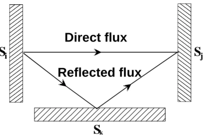
Among the various approaches for modeling radiative transfer within such enclosure [6], the absorption factors method is chosen. By definition, the absorption factor Bij between two surfaces Si and Sj represents the fraction of the energy emitted by Si that is absorbed by Sj. It is an "improved" view factor that takes into account all the optical paths from Si to Sj, whether the paths are direct or include reflections from the other surfaces Sk (Fig. 1). It thus depends on the radiative properties of all the surfaces (emissivities εi) and all the view factors Fij (which depend only on the geometry). The absorption factors Bij are deduced from Fij by solving the linear system [6-8] :
N ,..., 2 , 1 i ; B F F B ik kj N 1 k k ij j ij = +
∑
= = ρ ε (1)where (εjFij) is the fraction of the direct flux emitted by Si and absorbed by Sj,
( kj N k ik kF B
∑
=1ρ) is the fraction of the flux emitted by Si, reflected from other surfaces and then absorbed by Sj (ρk is the reflectivity for opaque gray-diffuse surface ρk = 1-εk).
Equation (1) can also be written :
[
]
j ij N k kj ik k ki ρ F B ε F δ − =∑
=1where δki is the Kronecker's symbol. The Bij matrix is then obtained by simple matrix inversion.
For the direct model, the net radiative fluxes between two surfaces are obtained from a set of boundary conditions given at each surface. If the assumption is made that the geometry, the surface emissivities and all the temperatures are known, the radiative net-exchange flux Qi,net for surface i can be expressed as follows:
N ..., , 2 , 1 i ; E B S E S Q ji b,j N 1 j j j i , b i i net , i = −
∑
= = ε ε (2a)where (Si
ε
iEb,i) is the energy emitted by Si, (Sjε
jBjiEb,j) is the part of energy emittedby Sj that is absorbed by Si.
Using the equations of reciprocity SiεiBij =SjεjBji and energy conservation
1 1 =
∑
= N j ij B , Eq.(2a) becomes :∑
∑
= = = − = = N j N j net ij j b i b ij i i net i i net i S q S B E E Q Q 1 1 , , , , ,ε
( ) (2b)The net-exchange flux Qij,net between two surfaces Si and Sj can then be written :
) ( , , , ,net i ijnet i i ij bi b j ij Sq S B E E Q = =
ε
− (3)The form of this expression is due to the work of Hottel [10] and was widely used for participating media. Equation (3) is considered as the product of an
“optico-geometrical” term SiεiBij (or total exchange area) and blackbody emissive power differences (Eb,i −Eb,j) (or a term relative to the temperature differences since
) ( 4 4
,
,i b j i j
b E T T
E − =
σ
− ). The analysis of the net-exchange rate matrix composed of the Qij,net values can highlight some “active surfaces”, from a radiative point of view,on a part or a whole of the human body [11]. Moreover, writing the radiative balance
net i
Q, as a discrete sum of net-exchange fluxes between two surfaces makes it possible
to determine the principal net fluxes and thus to establish a hierarchical order of radiative influence.
3. Formulation of the inverse problem
3.1. System of linear equations
The objective of the inverse model is to find the boundary conditions in the enclosure that will provide the given radiative environment on the human body for both
temperature and radiative flux, when the fluxes and temperatures of certain surface elements of the system are known. A difference then appears in the number of items of information associated with each surface. The surfaces can be classified in 4 categories [5] :
- nTF surfaces where the net flux and temperature are known (TF). - nT surfaces where only the temperature is known (T).
- nF surfaces where only the net flux is given (F). - nNS surfaces where nothing is specified (NS).
It has to be noted that as we are interested in the energy balance, the blackbody emissive power will be used rather than temperature as 4
T Eb =σ .
As shown in Fig.2, the inverse model requires prior knowledge of the geometry (Fij), the radiative properties (εi) (and thus the absorption factors Bij) and the boundary conditions of the surfaces T, F and TF, so that the unknown temperatures can be calculated.
The task here is to write the necessary equations so that the unknowns can be deduced from the known data.
In the method proposed here, Eq.(2b) is written for the surfaces where the net flux is known i.e. the TF and F elements. It is then necessary to solve a linear system in which the unknowns are the blackbody emissive powers Eb of the NS and F surfaces and the fluxes of the T surfaces (that do not appear in the solution vector explicitly). In this study, we chose to solve a system which contains as many equations as unknowns that implies the following condition:
nTF = nNS (4)
When all the equations have been written, it can be seen that only the equations
concerning the TF and F surfaces are needed to build the system. The equations for the T and NS surfaces are explicit for net fluxes and can be used in a second step if
necessary. The important conclusion of this observation is, although the set of equations has 2nNS+nF+nT unknowns, which are either blackbody emissive powers or net-radiative fluxes, the problem can be solved by considering only the blackbody emissive powers as unknown, i.e. with only nNS+nF unknowns. The size of the problem decreases from (2nNS+nF+nT) to (nNS+nF). The main interest of such a system of equations is to relate directly the design surfaces (human body), where two conditions are known, to the unknown blackbody emissive powers of the NS “driving surfaces” of the environment, and thus to avoid the radiosity calculation for all the surfaces.
A linear matrix system A E = b is then obtained which is composed of the following elements:
- a matrix A((nTF+nF), (nNS+nF)) relative to the geometry and radiative properties of the surfaces,
- the input vector b(nTF+nF), which depends on the information given for the TF, F and T surfaces,
- the solution vector E(nNS+nF) composed of the unknown blackbody emissive powers of the NS and F surfaces.
This formulation leads to a matrix A of smaller dimension than the matrix resulting from the radiosity method initially described by Harutunian [5] of dimension (N, N). 3.2. Regularization of the system of equations
Unfortunately, the A E = b matrix system obtained is known to be a linear discrete ill-conditioned system [3]. The computed solutions are sensitive to small perturbations of the inputs and the resolution of such a problem requires using specific mathematical methods such as regularization methods.
An inverse design problem can be solved satisfactorily only if additional constraints are applied to stabilize the original problem, which in turn introduces an error into the solution. In general, for increased levels of stabilization, there will be a greater error, which implies that a compromise is necessary. This is the basic idea of regularization methods [3].
Various regularization techniques suited to solve this type of problem have been studied by several authors [2]. Here the Tikhonov method is used, which consists of introducing a side constraint in order to stabilize or regularize the problem [9].
Instead of solving the ill-posed least squares problem (min AE−b 2), the solution can be obtained by calculating the single regularized solution to the minimization problem :
{
2}
2 o 2 2 2 E AE b L(E E ) min − +λ − (5)where L(E−Eo ) 22 is the side constraint, L is typically either the identity matrix or a
discrete approximation of a derivative operator, and allows the norm of the solution vector to be checked, Eo is an initial estimate of the solution. Eo=0 will be used for the rest of the study.
The regularization parameter λ needs to be chosen with a view to controlling the influence of the side constraint 2
2
LE . The case λ=0 corresponds to the least squares solution which is generally unacceptable.
According to Eq.(5), for larger λ, the solution is more regularized in the sense of
minimization of the side constraint. A small λ has the reverse effect. Thus, the selection of λ is an important part of the inverse solution and must be made carefully.
In our design problem, a solution is defined by its uniformity degree and its accuracy. - The accuracy of the solution is given by the difference between the required radiative heat fluxes on the design surfaces and the same net fluxes calculated from the inverse solution. An absolute error is then calculated for each design surface and compared to the precision required in the design.
- The uniformity degree of the solution describes the difference between
components of the vector solution E, which are the blackbody emissive powers of NS and F surfaces. For larger values of λ, the simultaneous effect of L and λ favors close components (and thus close temperatures), but at the expense of the residual error. The homogeneity of the solution is characterized by the standard deviation of the
surrounding temperatures.
The mathematical definition of these two physical constraints will be given in the section 4.4.
4. Application : radiative exchanges of a human body in a complex enclosure
4.1. Presentation
Human thermal comfort depends on the heat exchange with his/her environment. This paper focuses only on radiative exchanges that represent one of the main avenues for heat transfer between the driver and the car. The car thermal conditions are very non-uniform from several points of view : the temperatures of the walls, their radiative properties and their complex geometry.
Once seated at the wheel, the driver is exposed to various radiative sources such as a burning hot dashboard or ice-cold windows. The human body is constantly subjected to differences of temperature of the elements around him. It is for this reason that the calculation of its radiative exchanges is indispensable in the investigation of any thermal balance, even if this depends also on convective and evaporative exchanges. Those two last modes are taken into account through our thermoregulation model but are not the aim of this study.
The objective is to obtain a given radiative environment on the human being. The inverse model can determine the boundary conditions (temperatures) of the chamber capable of producing such an environment through inverse design. The thermal conditions that have to be reproduced are given by both flux and temperature of each
body segment. The solutions obtained by the inverse model are then tested and verified with the forward model.
4.2. Geometry
In comparison with previous studies [11], the geometry of the system (driver and his compartment) was simplified. The person and compartment have been divided into more than 500 plane triangular or quadrangular surface elements and the view factors Fij for the complex geometry are calculated by a Monte Carlo method.
The first difficulty was to reduce the number of surfaces for the inverse analysis. This large number of elements (500 surfaces) led us to group those with similar radiative properties and temperatures such as to obtain 22 isothermal panels or groups of surfaces to work with (Fig.3).
The first 7 panels describe the geometry of the human body and represented its major segments (head, trunk, right arm, left arm, hands, legs, feet). The other 15 are used for the description of the enclosure. All emissivities are fixed at 0.9.
The problem is stated as follows :
N=22, this is the total number of surfaces describing the geometry, including that of the human being.
nTF =7, these are the surfaces of the human body where both temperatures and fluxes are known.
There are thus 15 surfaces for which a boundary condition (temperature or flux) needs to be calculated. According to what has been established in the foregoing sections, the condition nNS = nTF =7 is made, which means that nT+nF =8. We suppose that there are no F surfaces for this study (nF =0). There is thus nT=8 surfaces of the enclosure for which the temperature had to be chosen a priori. This is one of the hypotheses of the problem. The nNS =7 temperatures to be calculated depend on this choice.
4.3. Temperatures and heat fluxes on the human body (design surfaces)
Many thermal environmental situations may procure thermal comfort for a human being, which depends on the thermal balance of the body in which each mode of heat transfer are encountered. To calculate the human body heat balance, our laboratory has been using a thermoregulation model for many years [12]. This model calculates the thermal state (temperature and heat fluxes) and thermal sensation, for the entire body and for each of the 7 segments according to the thermal external conditions and the physiological reactions.
In our large data base of real situations, we chose one situation where the global thermal sensation and the local ones are all neutral. The person is seated in a car, with low activity corresponding to driving and is dressed with summer clothing (note that the head and hands are naked). The thermal conditions are nearly constant so the driver can be considered to be at steady state. Both temperatures and fluxes are given by the model in table 1. It has to be noted that convective losses are low because the air is quite warm, the walls are colder than the air thus radiation represents 46% of the global heat losses on body surface. The conditions that have to be reproduced correspond to the two last lines of the table (local surface temperatures and radiative fluxes).
The temperatures of T surfaces are equal to the air temperature measured in the cockpit and are fixed to 29°C.
4.4. Accuracy and uniformity degree of the solution
Contrary to experiment-based problems, the designer using inverse methods is happy to have multiple solutions so long as they satisfy the prescribed design set within some prescribed error bounds and are physically attainable. Multiple solutions allow the
designer a choice, and the solution that the least expensive and easiest to implement can be chosen from among them [3]. In this study, the designer aims at finding a set of useful solutions that can be directly implemented in the system according to practical limitations imposed by available structural components, etc. To be accepted, the
solution must satisfy two major conditions concerning accuracy and uniformity degree, which are the physical constraints.
Accuracy of the solution : Admissible solutions are obtained from regularization of the original system of equations. Therefore, they are necessarily approximations for the problem and need to be verified. Once the temperatures on the “driving surfaces” are obtained, a forward problem is then solved to compute the radiative heat fluxes on each element i of the human body (qinverse) and compared to the desired heat flux (qimposed) by:
i inverse i imposed i = q , −q , η
For this problem, the solution is chosen if the condition ηi <η0 is satisfied where η0 is
the precision required in the design. It defines a domain of admissible solutions. The value of
η
0 is taken as a reference value coming from previous thermophysiological works [13] and is fixed atη
0 =20W/m². To simplify the problem, the global parameterη is introduced by : 7 , 1 ) ( max = = ηi fori η or ∞ = ηi η
In other words, once η is calculated for the 7 body segments, the solution vector is admissible only if the inequality η<20W /m² is checked.
Uniformity of the solution :
For practical reasons, it is of interest to control the temperature difference between each surface of the enclosure. For example, a large temperature dispersion of the surrounding surfaces can leads to undesirable effects of natural convection. Moreover, the
temperatures should range between a given interval suited to the practical aspects. In that way, a derivative operator of order 1 is employed such as :
− − = = . . 1 1 1 1 1 L
L is a band matrix composed of –1 and 1. This operator favors
close blackbody emissive powers as the regularization parameter λ increases (Eq.5), but at the expense of the precision.
To characterize the degree of uniformity of the solution, the parameter δ is introduced. δ corresponds to the standard deviation of the temperatures of the surrounding surfaces. For low values of λ, the components of the vector E present step oscillation between large positive and negative numbers. On the other hand, the δ value decreases as λ increases, that induce a uniform solution.
The influence of these two physical constraints on the solution is controlled by the regularization parameter λ that must be chosen carefully. For a given specification, the designer then would be given a number of solutions with one to be selected based on precision and practicality.
5. Results and discussion
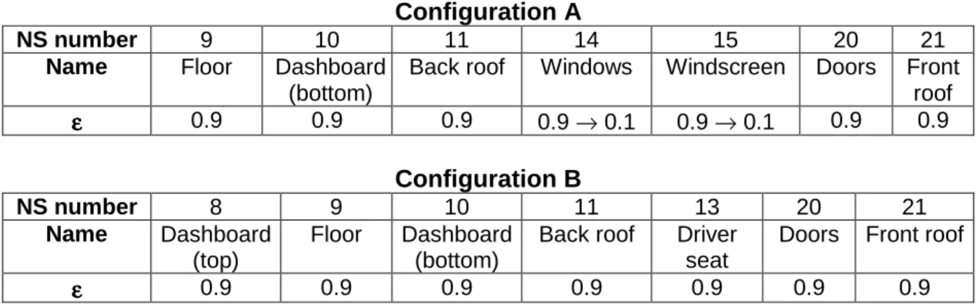
Before seeking solutions, the 7 “driving surfaces” of type NS must be chosen among the 15 walls of the cockpit. The glass surfaces are all assumed to be opaque boundaries, which is valid for the temperatures and characteristic long wavelength radiation considered here. Two configurations are studied :
- the first one (configuration A) comes from a physical analysis of the
problem. Indeed, surfaces NS are indicated according to their strong “optico-geometrical” influence on the whole of the human body i.e. present the highest total exchange area SiεiBij with the whole of the body. Both windows and windscreen belong to this list (Table 2).
- The second configuration (configuration B) is based on a practical choice of the NS surfaces which consists in taking surfaces able to be controlled in temperature within an automobile cockpit (Table 2). Windows and
windscreen do not belong to this list but the influence of their emissivity on the solution will be analyzed.
It was pointed out that 8 other surfaces of the enclosure (T surfaces) have their temperature fixed at 29°C. The results are presented in Table 3. Initially, all the emissivities are fixed at 0.9.
Configuration A :
As seen before, the solution characteristics depend on the λ value. The figure 4 shows the variation of the validation parameter ηi of each body segment i for 100 values of λ between 10-2 and 10. For this study, it is more interesting to analyze the behavior of the global parameter η (maximum of ηi) represented by circles. As expected, this maximum increases as λ increases but some solutions must be eliminated since they are not
physically acceptable or not suited to practical. For example, the solution corresponding to λ=0 is composed by negative blackbody emissive powers ! However, it is important to note that η is increasingly smaller than ηo=20 W/m² and so an admissible solution can be computed for each λ between 0.1 and 10.
The uniformity degree of the solution is represented by the parameter δ as shown in Fig.5. The temperatures become more uniform as λ increases until an asymptotic value close to 8°C. These results show that it is easily possible to calculate useful solutions that satisfy the required conditions. The space of solutions is represented on the 3D graph of Fig.6 for the right values of λ between 0.1 and 10. The temperatures calculated for low values of λ are more dispersed but more accurate. On the other hand, the
strongly regularized solutions (high λ) are more uniform but less accurate. The temperatures then tend to become closer as λ increases. Considering that the problem allows different solutions, as indicated in Fig.6, it is of interest to establish a set of criteria for the choice of an optimal solution depending on the designer’s objective. The graph of Fig.7 plots the degree of uniformity (δ) versus the accuracy (η) for each value of λ. This procedure is similar, from a physical viewpoint, to the L-curve method which allows to choose an optimal value for λ corresponding to the best trade-off between accuracy (η) and homogeneity (δ) [2]. For this example, the λ optimal value is
λo=0.7743 and the corresponding solution is represented in Table 3. The designer can then easily pick up an optimal solution from the plot of this graph (Fig.7).
Configuration B :
For this configuration, the behaviour of the λ and η parameters is close to the first configuration i.e. a large number of useful solutions can be obtained for many values of the regularization parameter. As seen previously, an optimal solution can be calculated
corresponding to an optimal value of λ (Fig.8). However, a high value of λo is obtained which minimizes δ. The blackbody emissive powers are thus very similar since the regularization method favours close components as λ increases. The temperatures of the NS surfaces corresponding to the λo value are close to 12°C with η=19.2 W/m² and
δ=8.8 °C.
It is of interest to note that the L-curve approach is not always the best choice to obtain useful solutions for this design problem; since non-physical solutions can be computed like negative blackbody emissive powers. Each situation is different and must be analyzed carefully.
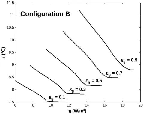
Influence of glass emissivities εg
It is of interset to study the influence of the glass emissivities (windows and
windscreen) on the accuracy and homogeneity in temperatures. The influence of glass emissivities on the inverse solution is shown on the Fig. 9 for the two configurations. - Configuration A : the problem is specific since both windows and windscreen are considered as NS surfaces. The smaller glass emissivities (and so the smaller
absorption factors), the less the influence that glass has on the human body. The optimal solution characteristics are then more appropriate when the glass emissivities are high (Table 3). Moreover, it is interesting to note that the condition number K(A) decreases as the glass emissivities increase.
- Configuration B : for small values of εg, both windows and windscreen become good reflectors of the cockpit and so the absorption factors between the NS surfaces and the human body (or total exchange areas) increase. Hence, the lower their emissivities, the more the radiative influence of NS surfaces on the human body. The optimal solutions become more appropriate to the designer’s objectives. For example, when glass emissivities are fixed to εg=0.1, the optimal corresponding solution (Table 3) presents more convenient values of η and δ than the initial configuration (εg=0.9). The range of the NS temperatures is higher than 12°C, which can be explained by the increase of the absorption factors between the NS and the TF surfaces.
5.2. Discussion
The results presented in the previous section illustrate an example of an inverse radiative design problem applied to human shapes. A methodology and some practical solutions have been presented for two given situations. The solutions obtained depend on the numerical parameters (λ, L) and also on the physical inputs (geometric and physical constraints of the enclosure). Many tests have been performed [14] concerning the sensibility of the solution to multiple parameters but only the influence of glass emissivities is presented here.
Another important feature of inverse design problems concerns the choice of the enclosure decomposition and how this choice affects the assumptions of uniformity. A small number of surrounding surfaces has been chosen first of all according to
technological problems, since the aim of this study is to build a climatic chamber to test the solution. An improved geometrical discretization of both the human being and the surrounding is possible, but actually only a reduce number of enclosure temperatures can be controlled. Subdividing into small surfaces while imposing that they have the same temperature implies that the problem will be overdetermined (more equations than temperatures to compute). But it has to be underlined that regularization methods are well suited to solve under or overdetermined systems [2-3].
It has to be noticed that the work presented here is a first step in this area, now that the tools have been developed, lot of work has to be done in testing all parameters. The
determination of an optimal geometrical discretization suited to the practical constraints that verify the physical assumptions is a future way.
6. Conclusion
This paper opens a new area in the design of human thermal environment by the use of inverse modeling. A methodology is presented here.
The work considers the inverse boundary design where the temperatures on some “driving surfaces” of the enclosure are determined that satisfy the specified temperature and heat flux on the human body. The conventional trial-error formulation is then avoided by using an inverse design approach that can directly compute a solution without iterations.
The physical formulation is described by the absorption factors method which leads to solution of a system of linear equations where the unknowns are the blackbody emissive powers. The system cannot be solved by conventional matrix solvers, requiring
regularization methods such as the Tikhonov method. A set of solutions is thus obtained and are discussed in terms of uniformity and accuracy of the results. A physically acceptable solution has then be chosen according to the designer’s objectives.
An improvement of this work would be make about the discretization of the geometry. Eventually, it will be possible to determine an optimal number of both the surrounding surfaces and the body segments that could fit best the assumption of uniformity and the practical constraints.
The next step in the research is to take into account the convective exchanges on the human being. This will require a simplification of the problem because of the complexity of convective transfers within such enclosure. In this way, it would be desirable to use a more sophisticated inverse model where convective effects could be introduced as boundary conditions to the radiative equations.
Acknowledgments
The authors would like to thank Prof. John R. Howell for helpful discussions and suggestions during the preparation of this work.
This study has been partly supported by PSA Peugeot Citroën.
References
[1] J.R. Howell, O.A. Ezekoye, J.C. Morales, Inverse Design Model for Radiative Heat Transfer, Journal of Heat Transfer 122 (2000) 492-502.
[2] P.C. Hansen, Rank-Deficient and Discrete Ill-Posed Problems, Numerical Aspects of Linear Inversion, SIAM Philadelphia, 1998.
[3] F.R. Franca, J.R. Howell, O.A. Ezekoye, J.C. Morales, Inverse Design of Thermal Systems, in : J.P. Hartnett, T.F. Irvine (Eds.), Advances in Heat Transfer 36, Academic Press, 2002.
[4] J.R. Howell, Recent Advances and Opportunities in Engineering Radiation Heat Transfer, in : Dinker Publishers (Eds.), Proceedings of the 15th National Heat Transfer Conference and 2nd ISHMT/ASME Heat and Mass Transfer Conference, Ahmedabad, India, 2000.
[5] V. Harutunian, J.C. Morales, J.R. Howell, Radiation exchange within an enclosure of diffuse-gray surfaces : the inverse problem, Proceedings of the 30th
[6] R. Siegel, J.R. Howell, Thermal Radiation Heat Transfer, 4th ed., Taylor and Francis, New York, 2002.
[7] B. Gebhart, Heat Transfer, Mc Graw-Hill, New York, 1961.
[8] E.M. Sparrow, On the calculation of radiant interchange between surfaces, Modern Developments in Heat Transfer, Academic Press, New York, 1963, pp. 181-212.
[9] A.N. Tikhonov, V.Y. Arsenin, Solution of Ill-Posed Problems, V.H. Winston & Sons, Washington, D.C, 1977.
[10] H.C. Hottel, A.F. Sarofim, Radiative Transfer, Mc Graw-Hill, New York, 1967. [11] G. Leduc, F. Monchoux, F. Thellier, Analysis of human’s radiative exchange in a complex enclosure, Proceedings of Moving Thermal Comfort Standards into the 21st Century, Windsor, UK, 2001.
[12] F. Thellier, A. Cordier, F. Monchoux, The analysis of thermal comfort
requirements through the simulation of an occupied building, Ergonomics 37 (5) (1994) 817-825.
[13] www.espace-elec.com/promodul/
[14] G. Leduc, Analyse directe et inverse des échanges radiatifs : application à une enceinte habitée, PhD thesis, Université Paul Sabatier, Toulouse, France, 2003.
Figure captions
Fig.1 : Optical paths between surfaces
Fig.2 : Principles of the inverse radiative problem
Fig.3 : Simplified representation of driver’s compartment
Fig.4 : Variation of the η parameter for 100 values of λ (configuration A) Fig.5 : Variation of the δ parameter for 100 values of λ (configuration A) Fig.6 : Inverse solutions obtained for 100 values of λ (configuration A) Fig.7 : Determination of the λ optimal value for configuration A (εg=0.9) Fig.8 : Determination of the λ optimal value for configuration B (εg=0.9) Fig.9 : Influence of glass emissivities εg
Direct flux
Reflected flux
S
iS
jS
kF
ijεεεε
Geometry Radiative properties T surfacesT
TF, q
TFq
FT
T TF surfaces F surfacesInverse model
Known
parameters
Unknown
variables
T
NS, q
NS Boundary conditions of NS surfaces Other boundary conditionsT
F, q
TF
ijεεεε
Geometry Radiative properties T surfacesT
TF, q
TFT
TF, q
TFq
FT
T TF surfaces F surfacesInverse model
Known
parameters
Unknown
variables
T
NS, q
NST
NS, q
NS Boundary conditions of NS surfaces Other boundary conditionsT
F, q
TFig.2 : Principles of the inverse radiative problem
T = ?
T = ?
T = ?
T = ?
T = ?
(qnet, T) desiredNumber of surrounding surfaces = 15 Number of body segments = 7
T = ?
T = ?
T = ?
T = ?
T = ?
(qnet, T) desiredNumber of surrounding surfaces = 15 Number of body segments = 7
10-2 10-1 100 101 0 2 4 6 8 10 12 14
λλλλ
ηηηη
(
W
/m
²)
ηηηη
Unacceptable solutionsηηηη
i i=1,7 10-2 10-1 100 101 0 2 4 6 8 10 12 14λλλλ
ηηηη
(
W
/m
²)
ηηηη
Unacceptable solutionsηηηη
i i=1,7Fig.4 : Variation of the η parameter for 100 values of λ (configuration A)
10-2 10-1 100 101 8 9 10 11 12 13 14
λλλλ
δδδδ
(
°C
)
Unacceptable solutions10-1 100 101 9 10 11 14 15 20 21 8 10 12 14 16 18 λλλλ NS number T e m p e ra tu re ( °C )
Fig.6 : Inverse solutions obtained for 100 values of λ (configuration A)
6 7 8 9 10 11 12 13 8 8.1 8.2 8.3 8.4 8.5 8.6 ηηηη (W/m²) δδδδ ( °C ) λoptimal value
13 14 15 16 17 18 19 20 8.5 9 9.5 10 10.5 11 11.5 ηηηη (W/m²) δδδδ ( °C ) λoptimal value
Fig.8 : Determination of the λ optimal value for configuration B (εg=0.9)
6 8 10 12 14 16 18 20 7.5 8 8.5 9 9.5 10 10.5 11 11.5 ηηηη (W/m²) δδδδ ( °C )
Configuration A
εεεεg= 0.1 εεεεg = 0.3 εεεεg= 0.5 εεεεg = 0.7 εεεεg= 0.96 8 10 12 14 16 18 20 7.5 8 8.5 9 9.5 10 10.5 11 11.5 δδδδ ( °C ) ηηηη (W/m²)
Configuration B
εεεεg= 0.1 εεεεg= 0.3 εεεεg= 0.5 εεεεg= 0.7 εεεεg = 0.9 6 8 10 12 14 16 18 20 7.5 8 8.5 9 9.5 10 10.5 11 11.5 δδδδ ( °C ) ηηηη (W/m²)Configuration B
εεεεg= 0.1 εεεεg= 0.3 εεεεg= 0.5 εεεεg= 0.7 εεεεg = 0.9Fig.9 : Influence of glass emissivities εg
Table captions
Table 1 : Human thermal characteristics
Table 2 : Description of the studied configurations
Table 3 : Optimal solutions characteristics obtained for two glass emissivities εg Temperatures : Mean skin: Tsk = 34.14 °C Mean body surface: Tcl= 29.45°C
Total heat flux :
Metabolic heat production : Qmet= 131.66 W Respiration Qresp= - 10.94 W
Convection : Qconv = -10.66 W Radiation Qray = - 44.24 W
Evaporation: Qevap= - 41.30 W
Global heat losses on skin surface Qtot = -96.21 W
Local data for each segment Head Trunk Left arm Right arm Hands Legs Feet Skin temperature (°C) Tsk(i) 36.12 33.70 33.40 33.53 35.91 34.21 33.88
Surface temperature (°C) Ts(i) 36.12 27.87 27.42 27.78 35.91 29.31 30.58
Radiative fluxes (W/m²) qnet(i) 103.72 36.59 28.08 30.03 96.14 37.82 49.88
Configuration A
NS number 9 10 11 14 15 20 21
Name Floor Dashboard
(bottom)
Back roof Windows Windscreen Doors Front roof εεεε 0.9 0.9 0.9 0.9 → 0.1 0.9 → 0.1 0.9 0.9 Configuration B NS number 8 9 10 11 13 20 21 Name Dashboard (top) Floor Dashboard (bottom)
Back roof Driver seat
Doors Front roof
εεεε 0.9 0.9 0.9 0.9 0.9 0.9 0.9
Table 2 : Description of the studied configurations
Configuration A NS surface Parameters εεεεg 9 Floor 10 Dashboard (bottom) 11 Back roof 14 Windows 15 Wind screen 20 Doors 21 Front roof K(A) λo η (W/m²) δ (°C) 0.9 15.4 14.4 13.5 12.9 12.6 12.5 12.2 193 0.77 7.7 8 0.1 15.2 12.5 10.8 9.8 9 8.3 7.3 420 0.53 9.9 9.7 Configuration B NS surface Parameters εεεεg 8 Dashboard (top) 9 Floor 10 Dashboard (bottom) 11 Back roof 13 Driver seat 20 Doors 21 Front roof K(A) λo η (W/m²) δ (°C) 0.9 12 12 12 12 12 12 12 76 >5 19.2 8.8 0.1 15.3 15.5 14.6 14 14 13.8 13.2 89 0.84 9.6 7.5