Use of the “Radiosity Importance Concept” in the Error Estimation in Radiative Heat Transfer Design of Spacecraft
Texte intégral
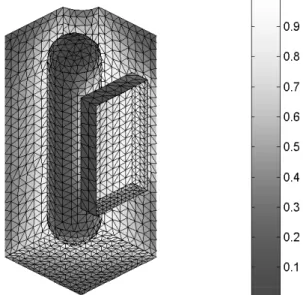
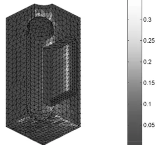
Figure
Documents relatifs
L’archive ouverte pluridisciplinaire HAL, est destinée au dépôt et à la diffusion de documents scientifiques de niveau recherche, publiés ou non, émanant des
Another interesting use of this controlled sequential exposure is the possibility to study the binding of a fluores- cently labeled protein to actin filaments, without using TIRF
Using regional regression trees, these data were calibrated to burned area estimates derived from 500-m MODIS imagery based on the conventional assump- tion that burned area
The outcomes of the previous results of Cases 1 to 4 are also applicable Case 6: The morphology affects the radiative heat transfer when the absorption of one species is not
La veille scientifique porte également sur la conservation des collections, activité dans laquelle les expériences conduites au sein d’autres musées sont toujours observées dans
L’archive ouverte pluridisciplinaire HAL, est destinée au dépôt et à la diffusion de documents scientifiques de niveau recherche, publiés ou non, émanant des
Given the pole-on viewing angle (i ∼ 12 ◦ ), it is possible that our detected 35% optical scattered light around 89 Herculis in Paper I, is largely arising in an outflow.
(b)Variation of the total radiative heat transfer coefficient (summation of the contributions of the evanescent and propagative EM waves of s and p polarizations) as function of
