Magnetic Order and Disorder in the Frustrated Quantum Heisenberg Antiferromagnet in Two Dimensions

HAL Id: jpa-00247209

https://hal.archives-ouvertes.fr/jpa-00247209

Submitted on 1 Jan 1996

HAL is a multi-disciplinary open access

archive for the deposit and dissemination of

sci-entific research documents, whether they are

pub-lished or not. The documents may come from

teaching and research institutions in France or

abroad, or from public or private research centers.

L’archive ouverte pluridisciplinaire HAL, est

destinée au dépôt et à la diffusion de documents

scientifiques de niveau recherche, publiés ou non,

émanant des établissements d’enseignement et de

recherche français ou étrangers, des laboratoires

publics ou privés.

Magnetic Order and Disorder in the Frustrated

Quantum Heisenberg Antiferromagnet in Two

Dimensions

H. Schulz, T. Ziman, Didier Poilblanc

To cite this version:

H. Schulz, T. Ziman, Didier Poilblanc. Magnetic Order and Disorder in the Frustrated Quantum

Heisenberg Antiferromagnet in Two Dimensions. Journal de Physique I, EDP Sciences, 1996, 6 (5),

pp.675-703. �10.1051/jp1:1996236�. �jpa-00247209�

Magnetic

Order

and

Disorder

in the

Frustrated

Quantum

Heisen-berg

Antiferromagnet

in

Two

Dimensions

H-J-

Schulz

(~,*)

T-A-L- Ziman

(~)

and D- Poilblanc

(~)

(~) Laboratoire de

Physique

des Solides

(**)

,

Universitd

Paris-Sud,

91405

Orsay,

France

(~) Lal~oratoire de

Physique

Quai~tique (**),

Universit6 Paul

Sabatier,

31602

Toulouse,

France

(Received

13 October 1995, received in final form 11 January1996,

accepted

22

January1996)

PACS.75.10.Jm

Quantized

spin

models

PACS.75.40.Mg

Numerical simulation studies

Abstract. We have

performed

_a numerical investigation of the

ground

state

properties

of the frustrated quantum

Heisenberg

antiferromagnet

_on the _square lattice

("Ji

J2

model"),

using

exact

diagonalization

of finite clusters with 16, 20, 32, and 36 sites.

Using

_a finite-size

scaling analysis

_we obtain results for a number of

physical

properties:

magnetic

order parameters,

ground

state energy, and

magnetic

susceptibility

(at

q =

0).

In order to assess the

reliability

of

our calculations, we also investigate

regions

of parameter space with well-established magnetic

order, in

particular

the non-frustrated case J2 < 0. We find that in _many cases, in

particular

for the intermediate

region

0.3 <

J2/Ji

< 0.7, the 16 site cluster shows anomalous finite size effects.

Omitting

this cluster from the

analysis,

_our

principal

result is that there is N6el type

order for

J2/Ji

< 0.34 and collinear magnetic order

(wavevector

Q

=

(0, ~))

for

J2/Ji

> 0.68.

An _error

analysis

indicates uncertainties of order ~0.04 in the location of these critical values

of J2. There thus is

a region in parameter space without any form of

magnetic

order. For the

unfrustrated case the results for order parameter,

ground

state energy, and

susceptibility

agree with series

expansions

and quantum Monte Carlo calculations to within a percent or better.

Including

the 16 site cluster, or

analyzing

the

independently

calculated

magnetic

susceptibility

we also find a

nonmagnetic

region,

but with modified values for the range of existence of the

nonmagnetic

region.

From the

leading

finite-size corrections

we also obtain results for the

spin-wave

velocity

and the spin stiffness. The

spin-war,e velocity

remains finite at the

magnetic-nonmagnetic

transition, _as

expected

from the nonlinear

sigma

model

analogy.

1. Introduction

In this _{paper we} consider _a

simple

example

of

quantum

frustrated

antiferromagnetism,

namely

the frustrated

spin-1/2

Heisenberg

model,

with Hamiltonian

H

=

Ji

~

_Si

_Sj

₊

J2

~

Si

Sj,

(1)

fi,Jl fi,J'l

The

spin

operators

obey

Si

Si

=

3/4,

and

Ji

" 1

throughout

this paper. The notations

(I,j)

and

(I,j')

indicate summation over the nearest- and next-nearest

neighbor

bonds on a square

(*)

Author for

correspondence

(e-mail:

heinz@solrt.lps.u-psud.fr)

(**)Laboratoires

assoc16s au CNRS

lattice,

each bond

being

counted once. While the model has attracted most attention as a

simplified

model

ill

of the effects of

doping

on copper oxide

planes

in the

high-temperature

superconducting

copper

oxides,

it is of rather more

general

interest. A

complete

understanding

would

provide

_a clear

example

of _answers to several

general

questions

about

quantum

phase

transitions.

The first

question

is that even in a

ground

state with rathe1classical

looking

symmetry,

in this

case an

antiferromagnet,

how do we show

unequivocally

that the order

really

is of

long

range

and not

simply

local? How do _we calculate

physically

measurable correlations without

relying

on low order

perturbation

theory?

In the present case, for small frustration the appearance, in

the limit of infinite

size,

of

spontaneous

symmetry

breaking

is

displayed

in _a

relatively simple

model. Indeed the renewed interest in the model was because of doubts that the unfrustrated

case would

display

long-range

order in the

thermodynamic

limit. While such doubts are now

relatively

_rare thanks to extensive numerical calculations and

tighter

rigorous

liniits for

higher

spin

and lower

spin

symmetry,

[2j there is as

yet

no

rigorous proof

for the

isotropic

spin

one-half

model in two

spatial

dimensions. One reason for the present

study

is to test the

quantitative

success of ideas of finite size

scaling

as

applied

to numerical

diagonalizations

that are

perforce

limited to what seem

unhelpfully

small

samples.

The

history

of finite size effects _goes back to Anderson in the

nineteen-fifties,

_[3j who first

invoked the fact that the infinite

degeneracy

of the

ground-state

with

spontaneously

broken

continuous

symmetry

must be manifest in _a

large

number of

nearly

degenerate

states in _a

large

but finite

system.

This idea of _a "tower" of states whose

degeneracy

corresponds

to the

ultimate

symmetry,

and whose _energy scales determine the

long

distance

parameters

of the

spontaneously

broken model of the infinite system has since been made more

precise

and less

dependent

_on

perturbative

concepts in the

language

of non-linear

sigma

models

[4j.

The model

we consider here has the

advantage

over, for

example,

the

triangular

or

KagomA

antiferromag-nets

[5,6j

in that the classical limit has _a

simpler

unit cell and thus the structure of the towers

should be

simpler

to test. One of _our aims here will be to show that it is

possible

to extract the

parameters

of the

long wavelength physics

in the ordered

regime.

In

practice

the difficulties of

applying

finite size studies _are still considerable: there _are

subleading

_as well as

leading

cor-rections which make the ultimate

goal

of reliable

quantitative

calculations difficult _even here.

It is

helpful

that _{we may}

easily

stabilize the ordered state to

study

the

disappearance

of order

in _a controlled fashion

by applying

negative

J2.

A second

general

question

relevant to other quantum

phase

transitions,

is whether the finite

Size methods

developed

_can be

applied

all the _way to a critical

point

at which the order may

disappear

with _a continuous transition. The first

step

is to

identify

the

parameter

J2c

of

this critical

point

unequivocally;

even its existence is still a matter for contention. Indeed

some self-consistent

spin-wave

expansions

have been

interpreted

as

indicating

a first order

transition

[7-9j,

at least for

large

spin.

We shall present results which _we feel _are rather

convincing

as to the existence of a critical

point

and a

reasonably

accurate estimate of its

value.

A third

question,

separate

from the

study

of ordered

antiferromagnetism,

is the

question

of

what

happens

when this order

disappears.

In the

mapping

of

quantum

interacting

ground

states

to

thermodynamics

of classical models in

higher

dimension,

there is at first

sight

a difference in

that quantum

phase

transitions tend to show order-order rather than order-disorder transitions.

Of _course what one means

by

"order" is crucial to such a distinction. Here an ordered state

would be understood to have

long

_range order in _a different local order

parameter,

for

example

a

spin-Peierls

dinierization variable or

chirality

parameter.

In this paper we do not discuss

in detail the nature of the intermediate

state,

but we do

produce

evidence that at least it

=16 .

2. Numerical Procedures and Results

We wish to find

eigenvalues

and

eigenvectors

of the Hamiltonian

ii

on

large

clusters. In order

to achieve

this,

and

given

that

computational

_power is and will remain

limited,

it is _necessary

to use the

symmetries

of the

problem

to reduce the size of the

corresponding

Hilbert space as

much _as

possible.

For the N

=

16,

32,

36

clusters _{we use:}

1, translational

symmetry

IN

operations

for an N-site

cluster).

2. reflection _on horizontal

(R-)

and vertical

(Rj)

axes

(4

operations).

For the N = 16 and

N

= 36

cluster,

both

symmetry

axis pass

in between _rows of

spins.

However,

for N

=

32,

the R--axis coincides with the central _row of

spin

(see Fig.

1).

3. if _a

given

eigenstate

has the _same

eigenvalue

under R- and

Rj,

then reflection _on the

diagonal

running

from the lower left to the _upper

right

of the cluster

(RI)

is also a

symmetry

operation,

and _can be used to further reduce the size of the Hilbert _space

by

a factor 2. For the 32 site cluster, this

operation

has to be followed

by

a translation to

remap the cluster onto itself.

4. if the

z-component

Sz

of the

total'magnetization

(which

commutes with the

Hamiltonian)

is _zero, then the

spin

inversion

operation

I)

-

i)

is also a symnietry and leads to

a further reduction

by

a factor 2. In

principle

a further considerable reduction of the

Hilbert _space could be achieved

by using

the conservation of the total

spin

S~.

However,

there does not seem to be any

simple

way to

efficiently

incorporate

this

symmetry.

The

point

group

operations

Id,

R-,Rj,

RI

generate

the

point

group

symmetry

C4u.

These

operations

are

only compatible

with the translational

symmetry

for states of momentum

Q

" 0

or

Q

"

(~r,~r).

In

particular,

for our clusters the

ground

state is

always

at

Q

= 0. For the

20 site clusters reflections _are not

symmetry

operations,

and _{we use} rather _a rotation

by ~r/2

as

generator

of the

point

group. The

symmetry

group at the

interesting

momenta

Q

= 0 or

Q

" (~r,~r) then is

C4.

We _{use a} basis set characterized

by

the value of

Szi

at each lattice site _i. An _up

(down)

spin

is

represented

by

a bit

(0)

in a

computer

word.

Thus,

a

typical spin

configuration (e.g.

for

a linear

system

of 4

spins)

would be

represented

as

iiii)

=

l1012

= 13

(3)

To

implement

the

symnietry,

we do not work in this

basis,

but use rather

symmetry-adapted

basis states.

E-g-

to remain in the one-dimensional

toy

example,

instead of

(3)

we use the

normalized basis state

jjj

iiii)

+

iiii)

+

iiii)

+

iiii))

=

jjj13)

+

j14)

+

j7)

+

iii))

e

j7)

(4)

where the lowest

"minimal")

integer

of the 4 states

occurring

in

(4)

is used to

represent

the state.

Our

procedure

to determine

eigenvectors

and

eigenvalues

proceeds

in three steps:

I)

starting

from an

arbitrary

basis state of

given

symmetry and

Sz,

the whole Hilbert _space is

generated

by repeated

application

of the

Ji

part

of the

Haniiltonian,

and the basis set is

stored; it)

the

Hamiltonian matrix is calculated and stored in two

pieces,

c6rresponding

to the

Ji

and

J2 parts

of the

Hamiltonian;

iii)

the matrix is used in _a Lanczos

algorithm

to obtain

eigenvalues

and

Table I. The nitmber

of

states in the Hiibert space

(nh)

and the nitmber

of

nonzero

off-diagonal

matrix elements

(ne

) for

the ciitsters itsed in this _paper. The nitmbers _are

for

states

in the

AI

representation

(A

representation

for

N = 20

)

at momentitm

Q

= 0.

N _{ah ne}

16 107 3664

20

1,321

55,660

32

1,184,480

78,251,988

36

15,804,956

1,170,496,152

of the Hamiltonian to a state

represented

by

a "minimal"

integer

will of course in

general

not

produce

another minimal

integer

state, but rather _a state that needs to be

brought

into

minimal form

by

the

application

of _a

symmetry

operation.

The trivial solution would be to

try

out all

possible

operations.

This however would be

extremely

time

consuming

(there

are

576

symmetry

operations

for the 36 site

cluster!).

Instead _{we use a} different

procedure

[15]:

the basis states are coded in a computer word so that the

Rj

operation

corresponds

to the

exchange

of the two halfwords. Each halfword then can be an

integer

between 0 and

2~/~

We

then create a list

specifying

for each

haifword

the

corresponding

minimal state

(integer)

and

the

symmetry

operation

(s)

connecting

them. The

length

of this list is

relatively

moderate _(2~~

at

worst),

and it _can be

easily

kept

in

computer

memory.

The minimal state

corresponding

to a

given

basis state is now determined

by

looking

in this

list for the minimal states

corresponding

to the two halfwords. If _necessary, the two halfwords

are

exchanged ii-e-

a

Rj

operation

is

performed),

so that the smallest of the two halfwords

constitutes the

high-bit

halfword of the

resulting

state.

Finally,

the

symmetry

operation

leading

to this

high-bit

halfword is

applied

to the

remaining

halfword. In about

80%

of the cases this

symmetry

operation

is

uniquely

determined. In the

remaining

_cases, more than one

symmetry

operation

has to be tried out in order to find the minimal state.

However,

the extra calculational

effort is

relatively

small: _e.g, for N

=

36,

only

for about a thousand out of 2~~

possibilities

are there more than

eight

symmetry

operations

to be tried out.

Using

this method for N = 36

the CPU time needed to calculate the basis set and the Hamiltonian matrix is

approximately

30 min and 90

min.,

respectively

[16].

For the smaller

clusters,

CPU time

requirements

are

obviously

much less. In Table I _we show the size of the basis set and the number of non-zero

matrix elements for states of

Ai

(N

=

16, 32,

36)

or A

(N

=

20)

symmetry

at

Q

" 0. These

are the

subspaces

containing

the

groundstate,

apart

from the case of

relatively large

J2

on the

N =

20,

36

clusters,

where the

ground

state has

point

group symmetry B

(N

=

20)

or

Bi

(N

=

36).

Note that the number of basis states for the

larger

clusters is very close to the naive

expectation

/~

/ji&N)

m 1.57554 x

io7

for N =

3&).

The number of matrix elements _e.g, for N

= 36 is still enormous. It is however obvious that

the matrix is

extremely

_sparse: on the average, there are fewer than 80 nonzero elements per

line,

which has in all

15, 804,

956

positions.

One

obviously only

wants to store the addresses

and values of the _nonzero matrix elements. This would still need two

computer

words per

non-zero matrix

element,

however,

this

requirement

can be further reduced

noting

that all matrix

elements are of the form

Hi,j

=

Ji,2 (Ii

/lj)f,j,

where the

Ii

are the normalization factors

of

the

symmetrized

basis states

(like

the factor

1/2

in

(4)),

and the

[,j

are small

integers,

which in

the vast

majority

of cases

equal unity.

More

specifically,

(

j

is the number of times the action

state

j)

or a state related to

j)

by

a

symmetry

operation.

The values of the

l~

intervening

in

a

given

matrix element can be

easily

determined

during

the

calculation,

and we thus

just

store

the

positions

of the unit

integer.

For the _cases where

[,j

= n

#

I,

the

corresponding

position

is stored _n times.

Finally,

a

Cray

computer word has 64

bits,

and therefore can accommodate

two addresses. In this way the whole matrix for the 36 site cluster can be stored in about

5

gigabytes,

which is

relatively easily

available _as disk _space at the

computing facility

we are

using.

Space

requirements

could be further reduced

by

a factor 2

using

the

symmetry

of the

Hamiltonian

matrix,

however,

this would have lead to a rather

important

loss of

speed

in the

subsequent

matrix

diagonalization.

To obtain the

groundstate eigenvalue

and

eigenvector

of the Hamiltonian _we use the standard

Lanczos

algorithm,

implemented

by

the Harwell

library

routine EAISAD. This routine

performs

rather extensive _convergence checks and _we thus avoid to

perform

unnecessary

time-consuming

Lanczos iterations. The main

problem

at this level is the use of the still rather

large

matrix

(ci

5

gigabytes).

The matrix

clearly

does not fit into the main _memory of _a

Cray-2 (2

gigabytes).

We therefore store the matrix on

disk,

and read it in

by

relatively

small

pieces,

whenever a new

piece

is needed. This

operation

can be made

computationally

efficient

by

using

"asynchronous"

input

operations,

which allow one to

perform

calculations in

parallel

with the read-in

operation

for the next

piece

of the matrix.

Moreover, using

_more than _one

input

channel

simultaneously

the read-in

operation

can be further accelerated. In this way the total time

overhang

due to

the continuous read-in of the matrix can be

kept

below

20%

of total CPU time. To reach

a relative accuracy

of10~~

for N =

36,

we need between 40 min.

(J2

"

0)

and 3 hours

(J2/Ji

QS

0.6,

slowest

convergence)

CPU time. We have

performed

a number of checks to

insure the correctness of the numerical

algorithm.

The most

important

one is to calculate the

groundstate

_energy for

ferromagnetic

interaction

(Ji,2

<

0),

which of course is known to be

(Ji

₊

J2)N/2.

However,

the numerical calculation in the

Sz

= 0

subspace

is nontrivial because

the Hilbert _space

and,

_up to an overall minus

sign,

the matrix are of course the same as for

the

antiferromagnetic

case. We also

compared

our results with

previous

finite size calculations

[17-21) (for

N

=

16,

20,

32)

and

quantum

Monte Carlo results

[22j

(for

N =

36, J2

=

0),

and

found

agreement

in all _cases.

Finally,

an

independent

check of the numerical accuracy of the

Lanczos

algorithm

is

provided by starting

the Lanczos iterations with different initial vectors.

In each _{case we} found a relative accuracy of at least

10~~

for the

ground

state

eigenvalues.

Similarly,

expectation

values calculated with the

eigenvector

are found to have relative accuracy

of

10~~.

In Table II we list

ground

state

energies

of the different clusters for a number of values

of

J2.

A _more

complete

set of results is

displayed

in

Figure

2.

More

important

for the

following

analysis

_are the values of the

Q-dependent

magnetic

sus-ceptibility

(or

squared

order

parameter)

1

~jjs

_.

)e~~'~~~ '~ ~~

Following

arguments

by

Bernu et _{al. [5]} we use a normalization

by

a

prefactor

_~j

(

~~ instead

of the usual

I/N~.

In the

thermodynaniic

limit,

these

possibilities

_are

obviously

equivalent.

However,

for the

relatively

small cluster _{we are}

using,

there _are sizeable differences in the

results of the finite-size

scaling

analysis.

The choice in

equation

(5)

is

essentially

motivated

by

the fact that in a

perfect

NAel state

M((Q)

is

entirely

size-independent

[23].

More

generally,

this choice eliminates _{to a} certain extent the

overly

strong

contributions from the terms with

I

=

j

in

equation

(5).

Some values of

fiI((Q)

_are shown in Table

III,

and

complete

curves are in

Figure

3. The

Table II. The

groitnd

state energy per site

for

different

ciitsters and

different

uaiites

of

J2

(Ji

is normalized to

itnity).

Where the

ground

state

representation

changes

with

increasing

J2

(N

=

20,

36),

the

energies

of

both relevant

representations

are

given.

Boldface

indicates the

approximate

location

of changes

in the

groitnd

state

symmetry.

J2

16

20(A)

20(B)

32

36(Ai)

36(Bi)

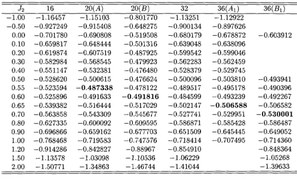
-1.00 -1.16457 -1.15103 -0.801770 -1.13251 -1.12922 -0.50 -0.927249 -0.915408 -0.648275 -0.900134 -0.897626 0.00 -0.701780 -0.690808 -0.519508 -0.680179 -0.678872 -0.603912 0.10 -0.659817 -0.648444 -0.501316 -0.639048 -0.638096 0.20 -0.619874 -0.607519 -0.487925 -0.599542 -0.599046 0.30 -0.582984 -0.568545 -0.479923 -0.562283 -0.562459 0.40 -0.551147 -0.532381 -0.476480 -0.528379 -0.529745 0.50 -0.528620 -0.500615 -0.476624 -0.500096 -0.503810 -0.493941 0.55 -0.523594 -0,487338 -0.478122 -0.489517 -0.495178 -0.490396 0.60 -0.525896 -0.491633 -0.491816 -0.484599 -0.493239 -0.492267 0.65 -0.539382 -0.516444 -0.517029 -0.502147 -0.506588 -0.506582 0.70 -0.563858 -0.543309 -0.545677 -0.527741 -0.529951 -0.530001 0.80 -0.627335 -0.600092 -0.609595 -0.586871 -0.585428 -0,586487 0.90 -0.696866 -0.659162 -0.677703 -0.651509 -0.645445 -0.649052 1.00 -0.768468 -0.719583 -0.747576 -0.718414 -0.707495 -0.714360 1.20 -0.914286 -0.842827 -0.88967 -0.854910 -0.848364 1.50 -1.13578 -1.03098 -1,10536 -1.06229 -1.05268 2.00 -1:50771 -1.34863 -1.46744 -lA1044 -1.39633

Table III. The normalized

sitsceptibiiity

(Eq. (5))

at

Q

= (~r,~r) and

Q

= (~r,

0) for different

ciitsters and

different

vaiites

of

J2/Ji.

M(~r,~r)

M(~r,0)

J2/Ji

16 20 32 36 16 20 32 36 -1.00 0.26924 0.26002 0.24296 0.23943 0.02778 0.02273 0.01470 0.01316 -0.50 0.26297 0.25221 0.23131 0.22660 0.02780 0.02273 0.01471 0.01316 0.00 0.24580 0.23430 0.20621 0.19879 0.02789 0.02278 0.01476 0.01322 0.10 0.23853 0.22785 0.19745 0,18893 0.02798 0.02284 0.01480 0.01326 0.20 0.22811 0.21949 0.18616 0.17601 0.02818 0.02292 0.01489 0.01335 0.30 0.21212 0.20816 0.17090 0.15800 0.02868 0.02309 0.01506 0.01354 0.40 0.18589 0.19193 0.14887 0.13109 0.03031 0.02348 0.01545 0.01404 0.50 0,14236 0,16693 0,11487 0.09236 0.03709 0.02452 0.01669 0.01594 0.55 0.11276 0.14834 0.09165 0.07062 0.04771 0.02621 0.01880 0.01965 0.60 0.07819 0.02915 0.05113 0.04378 0.07154 0.11508 0.04627 0.03822 0.65 0.04290 0.02015 0.01692 0.01954 0.10897 0.12615 0.10333 0.08167 0.70 0.02092 0.01303 0.01161 0.01232 0.13598 0.13461 0.l1321 0,10006 0.80 0.00721 0.00561 0.00520 0.00611 0,15407 0,14383 0.12265 0,11370 0.90 0.00374 0.00302 0.00251 0.00314 0.15930 0.14759 0.12616 0,11925 1.00 0.00236 0.00193 0.00147 0.00183 0.16164 0,14944 0.12759 0,12183 1.20 0.00126 0.00103 0.00072 0.00088 0.16379 0.lsl18 0.12876 0.12418 1.50 0.00067 0.00055 0.00037 0.00044 0.16507 0.15227 0.12939 0,12553 2.00 0.00033 0.00027 0.00018 0.00021 0,16586 0.15295 0,12977 0,12637

xxx% O-O

~x*"

~~

x +~ ~ ~

~~+~

h, ~ +

/~

'+ x ~ / ' _l''

_~+,

/ / ' -o.5 ~+/ / ~

II

~

',

'h

, x / / ' ~ ~ / / '

'~

~ / ~ ~ "

',

/ ' , / , -l.0

',

' ' ' ' -1.5

-1.0 -o.5 o-o o.5 1-o 1.5 z-o

Jz/Ji

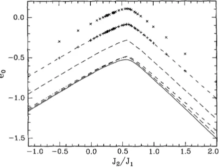
Fig.

2. The

ground

state _{energy per} site as a function of

J2/Ji

for N = 16

(full

line),

N = 20

(dashed

line),

N

= 32

(dash-dotted

line),

and N = 36

(dotted line).

For clarity, the curves for

N

= 20, 32, 36 are also

displayed

shifted

upwards by

0.2, 0A, and 0.6,

respectively.

For N = 16, 20 we

have results for

J2/Ji

in steps of 0.01, and

only

_a continuous curve is

displayed.

For N = 32, 36, we

have only results at the

points

indicated, and lines _{are a}

guide

to the _eye.

ground

state, e-g- for

large J2

states of

symmetry

B

(N

=

20)

or

Bi

(N

=

36)

are used. From

the results shown it is

quite

obvious that the dominant type of

magnetic

order

changes

from

Q

" (~r,~r) at

relatively

small

J2

(Ndel

state)

to

Q

= (~r,

0)

at

larger

J2

(collinear state).

How

exactly

this

change

_occurs will be clarified in the

following

section.

3. Finite-Size

Scaling

Analysis

3. I. ORDER PARAMETERS. The results shown in

Figure

3 show _a transition between _a N4el ordered

region

for

J2

$

0.5 to a state with so-called collinear order

ii-e-

ordering

wavevector

Q

" (~r,

0))

at

J2 2

0.6. To

analyze

the way this transition occurs in more

detail,

we use

finite-size

scaling

arguments

[24].

In

particular,

it is

by

_now well established that the

low-energy

excitations in _a NAel ordered state are well described

by

the nonlinear

sigma

model. From this

one can then derive the finite-size

properties

of various

physical

quantities.

The

quantity

of

primary

interest here is the

staggered

magnetization

mo(Qo)

defined

by

mo(Qo)"2

lim

MN(Qo)

,

(6)

N-m

where

Qo

"

(~r,~r).

The normalization is chosen so that

mo(Qo)

" in a

perfect

NAel state.

0.30 o,z5

~~~~~---_

~~~~~it-,

~~~~,

'~,

o,zo

t~+

p

©~

~

°'15

i~,

'I

~

j

~ o-lo o.05 ., ~'~~ -l.0 -0.5 0.0 0.5 1.0

12/li

a)

o.zo o,15 _

_++~-j---(---~ / x X

~

Q-IQ

"~

~i 0,05 ' ~_~ z-o

°.°°o.o

°.~

j~)~~

~

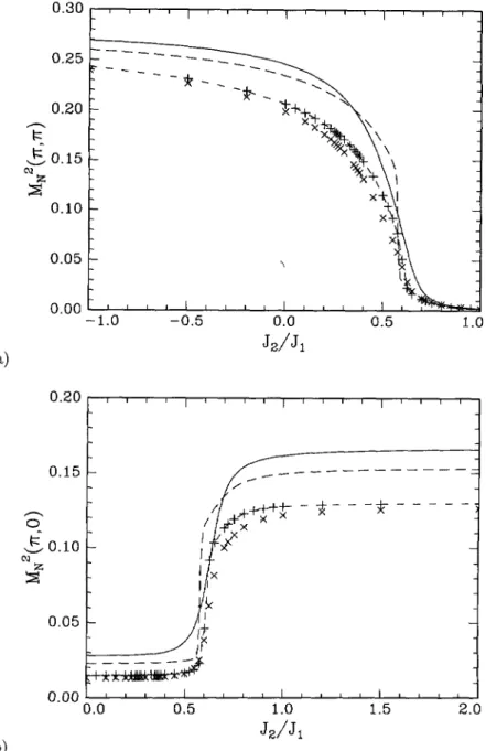
Fig. 3. The magnetic

susceptibility

M(Q)

at

a)

Q "

(~, ~)

and

b)

Q "

(~, 0).

The

symbols

and

linetypes are the same as in Figure 2.

~~~~°~

_~~°~~°~~

~ ~'~~~~

~

~

=

~mo(Qo)~li+

~'~$~+..)

0.30 o

Jz/J~=o.o

°.25

(

(]~([l(1(

~ ~g

(~~((=~.~

/

j~

0.20 * ~~/~~"°'~ ~

j

_ / 0 ~ / /

£

o.15 ~ /

[

m ~ / ~ / ~ / z~ / ~ / ~ ~ 0.10 / ~ / ~ / / / / / o.05 II ~

°'°°0.00

0.05 0.10 0.15 0.20 0.25

~-i/2

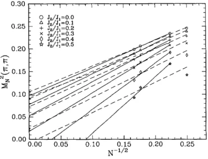
Fig.

4. Finite size results for

Ml

(Qo)

for different values of J2. The dashed lines _are least _squares

fits to the data

according

to

equation

(7),

using

all available clusters. The full fines _are fits

using

only

N

= 20, 32, 36. The dash-dotted line is the

leading

finite size behavior

expected

at J2 = o

(see

Eq.

(7)).

where for the infinite

system

~i

gives

the

amplitude

of the

diverging

matrix element of the

spin

operator

between the

ground

state and

single

magnon states at

Q

Ge

Qo.

Least _square fits of _our finite-size results to

equation

(7)

are shown in

Figure

4. For small

values of

J2

the

scaling

law is

quite

well satisfied: _e-g- for

J2

= 0 the four data

points

in

Figure

4 _very

nearly

lie _on the ideal

straight

line,

and the

extrapolated

value of the

stag-gered

magnetization,

_mu

(Qo)

"

0.649,

is

quite

close to the best current estimates

[22,

25-27],

mo(Qo)

= 0.615

[28].

Using

the same

type

of finite size

extrapolations

for other values of

J2,

we obtain the results indicated

by

a dashed line in

Figure

5.

For

J2

"

0,

a check on the

reliability

of our method can be obtained

by

comparing

the

numerical results with what _one would expect from

equation

(7), using

the rather reliable

results for _{mu, c,} and _ps obtained

by

series

expansion

techniques

[26,27,

29].

The curve

expected

from

equation (7)

is shown as a dash-dotted line in

Figure

4. It appears that there are sizeable

but not

prohibitively

large

next-to-leading

corrections.

Another measure of the

reliability

of the finite-size

extrapolation

can be obtained

comparing

results obtained

by

the use of different groups of clusters. For

negative J2,

I-e-

nonfnlstrating

interaction,

the values of

mo(Qo)

_are

nearly

independent

of the clusters sizes

used,

and the

results in

Figure

5 therefore _are

expected

to be

quite

accurate. In this

region

the next nearest

neighbor

interaction stabilizes the

antiferromagnetic

order and therefore the

staggered

mag-netization tends to its saturation value

unity

for

large

negative

J2.

On the other

hand,

for

positive

J2

the interaction is

frustrating.

In this case, the

agreement

between different

extrap-olations is less

good.

We note

however,

that in all but two cases the

staggered

magnetization

tends to zero as in a second order

phase

transition,

with a critical value of

J2

between 0.34

1-o o-B _ 0.6

Ci

O L=16,20,32,36

fl

6 L=20,32,36

~

+ L=16,32,36 0.4 X L=16,20,36 0 L=16,20,32 ~ * L=16,32 . L=16,36 + O-Z ~ +

~'~-Z.0

-1.5 -1.O -O.5 O-O 0.5

12/Jl

a)

o-B O N=16,20,32,36 ~ N=20,32,36 0 6

'I'

_.~

~=)~~(~~(~

- # ,

j

N=16,20,32 -'

~~~i~~h&j

=~~~~~

° . ++ ~k ~ A N=20 36 ~ 0 4 °.

)

°° ° ~ ~ . ~'x ~ 0 °. 'x _, . ~ , x' ~ + o-Z ~ . ' ~ +

'

~ + ~'~ o-O 0.Z 0.4 0.6 0.8

lz/li

b)

Fig.

5. The

staggered

magnetization

mo(Qo)

as a function of

J2/Ji

using

different combinations

of clusters

(a).

In

(b)

the "critical"

region

J2 > o is shown

enlarged.

clusters considered here is free of some

peculiarity:

for N = 16 and

J2

"

0,

there is an extra

symmetry,

because with

only

nearest

neighbor

interactions this cluster is in fact

equivalent

to

a 2 x 2 x 2 x 2 cluster on a four-dimensional

hypercubic

lattice;

the N = 20 cluster has a

lower symmetry than all the others

(C4

instead of

C4u)1

for N

= 20 and N = 36 the

ground

that

they

are

rotated,

by

different

angles,

with

respect

to the lattice directions. A

priori,

one

might

then argue that the best choice should be the least biased one,

including

all available

clusters. As indicated

by

the dashed line in

Figure

5,

this leads to _a critical value of

J2

for the

disappearance

of

antiferromagnetic

order of

J2c

* 0.48.

However,

from

Figure

4 it is

quite

clear that for

J2

> 0.35 the 16 site cluster is

highly

anomalous in that

M((Qo)

increases

going

to the next

bigger

cluster,

whereas in all other

cases there is a decrease with

increasing

size.

Clearly,

in

Figure

4 a much better fit is obtained

in this

region

by

omitting

the N = 16

results,

leading

to a reduced

value,

J2c

* 0.34 as

indicated

by

the full line in

Figure

5. The anomalous results obtained from the N =

16, 20, 32,

N

=

16, 32,

36 and N =

16,

32 fits are

certainly

due to an

over-emphasis

put onto the N = 16

results. Similar anomalous behavior of the 16 site cluster _occurs in _{many cases} in the

region

0.3 <

J2

<

0.8,

and we therefore consider the results obtained

using only

N =

20,

32,

36 as more

reliable. In

particular,

in this _way we find a

staggered

magnetization

of 0.622 at

J2

=

0,

only

about one

percent

higher

than the best current

estimate,

mo(Qo)

" 0.615.

Beyond

the

precise

value of the critical value

J2c

at which

antiferromagnetic

order

disappears,

the

important

result

here,

obtained

by

the

majority

of

fits,

is the existence of _a second order

transition,

located in

the interval 0.3 <

J2

< 0.5.

One

might

of _{course argue} that it is not the N = 16 but rather the N = 20 cluster that

is anomalous.

However,

closer

inspection

of the data in

Figure

4

clearly

shows that the

N

=

20, 32,36

data

points

remain

reasonably

well

aligned

even in the intermediate

region

0.3 <

J2

< 0.8, whereas the

alignment

for N

=

16, 32,

36 is much worse. The N =

20, 32,

36

fit also is

quite

stable:

omitting

either the N

= 32 or the N = 36

point

from it, one obtains

only relatively

small modifications in the results in

Figure

5. On the other

hand,

starting

from N

= 16.

32,

36 and

omitting

either of N = 32 or

N

= 36 leads to

strong

modifications.

Finally,

the N

=

16,20,32

fit

(which together

with N =

16,32,36

and N = 16,32 indicates a NAel

phase

_up to

J2

"

0.6)

also is unstable:

adding

N = 36 or

replacing

N = 32

by

N = 36 leads

to

drastically

modified results.

To obtain _a more

quantitative

criterion for the

quality

of the different

fits,

we use standard

methods of error

estimation,

as described for

example

in reference

[30].

The results for

M(

(Qo

in the

thermodynamic

limit N - co obtained from N =

16,20,32,36,

N =

20, 32,36,

and

N ₌

16,

32,

36 are shown in

Figure

6

together

with the

corresponding

variances [30]

represented

as error bars.

Extrapolations

using

other combinations of clusters lead to variances at least

twice as

big

as those for N =

16, 20, 32, 36,

and therefore are not discussed in the

following.

The

error bars have to be taken with some

caution,

because errors here

certainly

are not

normally

distributed but rather

systematic.

Nevertheless,

the relative size of the _error bars

certainly

is _a

significant

indicator of the

quality

of the fits. As to be

expected

from

Figure

4, the error bars for

the N

=

20, 32,

36 fit are

nearly

two times smaller than those obtained from the fit

including

all

points.

Similarly,

the total

x~

for N =

16, 20, 32,

36 and for N =

16, 32,

36 are

typically

twice as

big

and

30%

bigger

than the _one obtained from N

=

20,

32,

36. This rather

clearly

demonstrates

the

anomalously

large

error introduced

by

the N = 16 cluster.

Moreover,

one observes that for

the N

=

16,

20,

32,

36 and N = 16,

32,

36

fits,

the NAel order

disappears

in a

region

where the

error bars are

nearly

as

big

as the value of

M((Qo

at

J2

"

0,

indicating

a very poor

quality

of

the fit.

Only

for N

=

20, 32,

36 does the transition occur in a

region

of

relatively

small error bar.

Finally,

we note that at

J2

"

0,

we have

MS

(Qo)

= 0.105 ~

0.006,

0.097 +

0.004,

0,107+ 0.004

for N

=

16,20,32,36,

N =

20,

32,36,

and N =

16,32,36,

respectively,

whereas the best

current estimate for the

staggered

magnetization,

mo(Qo)

"

0.615,

leads to

MS

(Qo)

" 0.095.

Again,

only

the N

= 20.

32,

36

extrapolation

gives

consistent results. In the

follo~v.ing,

we

will

therefore

mostly rely

on the N = 20,

32,36

extrapolations.

From

Figure

6 we

then

expect

~'~~ i 0.25

~~~

~)j)~~~~

_ Q_zQ

~

§ ~ ~ ~

i

~/

_~j))

~ ~~

_~

j~

0.05 ~'~~

O-O O-I Q-Z O.3 O.4 O.5

12/li

Fig.

6. Results for the N _cxJ

extrapolation

of

M((Qi)

using

N

= 16, 20,32, 36

(circles),

N =

20, 32,36

(triangles),

and N

= 16, 32, 36

(crosses)

with error bars. For

clarity

the N = 20, 32,36 and

N

= 16,32, 36 results are shifted

upwards by

0.I and 0.2,

respectively.

estimate of 0.34. Similar

analyses

can also be

performed

for other

quantities

calculated below

(collinear

order

parameter,

_q = 0

susceptibility),

with similar results. We will therefore not

reproduce

this

type

of

analysis

in detail below.

We now follow the same

logic

to

analyze

the behavior for

larger

J2,

where

Figure

3

suggest

the

existence of

magnetic

order with

ordering

wavevector

Qi

" (~r,

0).

Of course, this state

again

breaks the continuous

spin

rotation

invariance,

and therefore the low _energy excitations are

described

by

a

(possibly anisotropic)

nonlinear

sigma

niodel. There is an additional

breaking

of

the discrete lattice rotation

symmetry

(ordering

wavevector

(0,

~r) is

equally

possible),

however,

this does not

change

the character of the

low-lying

excitations. The finite size behavior is

entirely

determined

by

the low _energy

properties,

and therefore we expect a finite size formula

analogous

to

equation

(7):

~~~~~~~

_j'~~o(Qi)~

+ ~~~~~'

+

~

(8)

Here the factor

1/8 (instead

of1/4

in

(7))

is due to the extra discrete

symmetry

breaking

which

implies

that finite-size

ground

states are linear combinations of a

larger

number of

basis states.

Moreover,

the nonlinear

sigma

model is

anisotropic,

because of the

spontaneous

discrete

symmetry

breaking

of the

ordering

vector, and

consequently

a

precise

determination

of the coefficient of the

I-term

is not

straightforward.

The

important

point

here is however

the

N-dependence

of the correction term in

equation

(8).

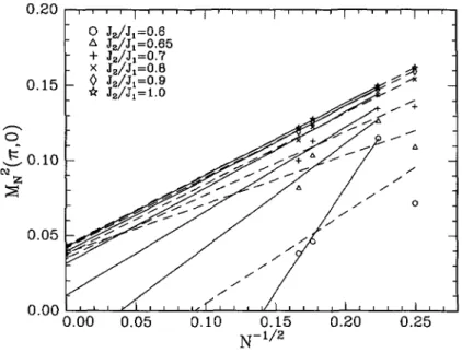
Least _square fits of our numerical results to

equation

(8)

are shown in

Figure

7,

and the

extrapolated

collinear

magnetization

mo(Qi)

is shown in

Figure

8. For

J2

> 0.8

equation

(8)

provides

a

satisfactory

fit to our

data,

even

though

not

quite

as

good

as in the

region

J2

< 0 in

o,zo O

J2/J~=o.6

6

J2/J~=o.65

+

12/J~=o.7

x

j~/j~=o.8

~$ 0 ~5 ~

~8/~~~~.~

~'~ *

Jz/J~=I.o

~ /~ /5

q

1' ~ _{o-lo ~} ' ~ m ~ / ~ / / / z~ / / / ° / o,05 / / / / /

°'°°0.00

0.05 O.10 0.15 0.20 0.25

~-i/2

Fig.

7. Finite size results for

M((Qi)

for different values of J2. The dashed lines _are least _squares

fits to the data

according

to equation

(8),

using

all available clusters. The full lines _are fits

using only

N

= 20,32,36.

region

J2

<

0).

For smaller

J2

there is a wide

spread

in the

extrapolated

results,

depending

on the clusters used. We notice however that for the

majority

of clusters

used,

there is a

common feature:

.mo(Qi)

remains finite down to

J2

=

o.65,

and then

suddenly

drops

to zero

at

J2

" 0.6. This would indicate a

first

order transition to the collinear state somewhere in

the interval 0.6 <

J2c

< 0.65. This

interpretation

also _seems consistent with the raw data

of

Figure

3: the increase of

M((Qi)

around

J2

" 0.6 is much

steeper

than the

growth

of

M((Qo)

with

decreasing

J2.

From the N

=

16,

20,32,36

extrapolation

one then obtains a

collinear

magnetization

which is

roughly

constant above

J2c

at

mo(Qi)

QS 0.6. Notice that

the first-order character of the transition is not due to the level

crossings

occurring

in the

N

= 20 and N = 36 clusters: if these clusters are omitted from the

extrapolation,

the first

order character is in fact

strongest

(cf. Fig.

8).

On the other

hand,

inclusion or not of the N = 16 cluster

plays~an

important

role because

this cluster shows

again

anomalous behavior in the

region

of intermediate J21 for

J2

< 0.7

M((Qi)

increases when N increases from 16 to

20,'contrary

to what

equation

(8)

suggests.

Indeed, an error

analysis

analogous

to the one

performed

for the NAel order

parameter

again

shows a much better

quality

of the N =

20,

32,

36 fit. If one therefore omits the N = 16 cluster

from the

extrapolation,

results

quite

consistent with a second order transition in the interval

0.64 <

J2/Ji

< 0.72 are

obtained,

with a best estimate for the critical

coupling

J2c/Ji

* 0.68.

It _appears that the collinear order

parameter

tends for

large

J2

to a value very close or

identical to that of the

antiferromagnetic

order _parameter at

J2

" 0. This is in fact not

difficult to understand: for

J2

>

Ji

our model represents two very

weakly

coupled sublattices,

with a

strong

antiferromagnetic

coupling

J2

within each sublattice.

Consequently,

the

ground

state wave function is to lowest order in

Ji

/J2

a

product

of the wavefunctions of unfrustrated

1.o

j

o-B t -0.6

I

~"

?

(

°.4 j. ~

=~~~~~~~~~~~

x N=16,20,36 0 N=16,20,32 j * N=16,32 °.~ 1°

~=~~~(~

A N=20,36 ~'~ O.5 1.0 1.5 Z-O

lz/li

a)

1-o ~ ~~ $~

~$

~ ++~ # , -0.6 +

?'

j

~

yG6s~~_~_

_~_-b--~~

~/ / .., ° ,

#

_/

°4'~

' _{O N=16,20,32,36} 0.4 p x 6 N=20,32,36 f > + N=16,32,36 x N=16,20,36 ' _N=16,20,32 > * N=16,32 Q-Z . . N=16,36 . N=2032 ' A

N=20~36

I

~'~O.5

_{O.6 0.7 O-B O-Q I-O}

lz/li

b)

Fig. 8. The collinear

magnetization

mo(Qi)

_as a function of

J2/Ji

using

different combinations of

clusters

(a).

In

(b)

the "critical"

region

0.5 < J2 <1.0 is shown

enlarged.

fiI(~~(Qo,

J2

"

0)/2,

and thus from

equations

(7)

and

(8)

we have the exact result

rim

mo(Qi)

=

mo(Qo)ll~)

J~ /J~-m

J~=o

uncer-8

~

~~

~

z

o

r

M

x

r

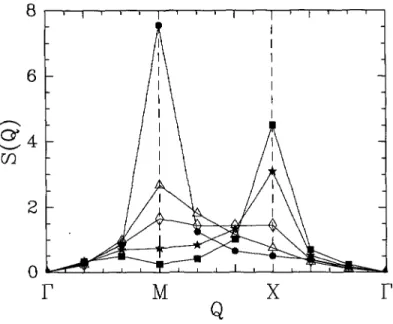
Fig.

9.

Magnetic

structure factor, as obtained from the N = 36

cluster,

in the Brillouin zone for

J2/Ji

" 0

(.),

0.55 (ZL), 0.6

(o),

0.65

(*),

1

(.).

The

points r, M,

X are

Q

= 0,

Qo, Qi,

respectively.

Note that nowhere there is

a maximum at a

point

different from M or X.

tainties. To obtain this

agreement

it was however crucial to use the normalization of

M((Q)

shown in

equation

(5). Using

_a factor

1/N~

instead we obtain for

large

J2

mo(Qi

*

0.4,

JA~hich

is far too low. The _reason for this is that _our

extrapolation

with N

=

16, 20, 32,

36

corresponds,

for

large

J2,

to a calculation on two

nearly

uncoupled

and unfrustrated

sublattices,

each with

N

=

8,10,16,18.

On such small

lattices,

short-range

effects are

obviously

rather

large,

and

therefore the _proper normalization of

M(

is

particularly

important.

Beyond

quantitative

results,

the most

important

conclusion of this

analysis

is the existence of a finite interval without

magnetic

long

range order: if all available clusters are included in

the

analysis,

this interval is 0.48

_£

_{J2 $}

0.6,

if,

because of the anomalies discussed above _one

omits the N

= 16

cluster,

the

nonmagnetic

interval is increased to 0.34

£ J2 £

0.68. The

study

of the

ground

state symmetry in this

region

requires

a detailed

analysis

of a number of

different

non-magnetic

order

parameters

and will be

reported

in a

subsequent

paper.

However,

at this

stage,

the

magnetic

structure factor

S(Q)

=

(N

+

2).lf(

IQ)

already gives

some valuable

information: in

fact,

as shown in

Figure

9,

with

increasing

J2

the collinear

peak

at the X

point

grows and the N4el

peak

at the M

point

shrinks,

however there never is a maximum at other

points.

There is thus _no evidence for incommensurate

magnetic

order.

3.2. GROUND STATE

ENERGY,

SPIN-WAVE

VELOCITY,

AND STIFFNESS CONSTANT, The

ground

state energy per site in the

thermodynamic

limit can be obtained from the finite-size

formula for an

antiferromagnet [4,24j

Eo(N)

IN

= eo

1.4372~

₊

,

(10)

where c is the

spin-wave

velocity.

Again,

in the collinear state, an

analogous

formula

holds,

-0.45 O -0.50 -+ x ~ 0 -O.55 * SS '

/

-O.60

~f

-O.65 -o.70 -O.75

O.OOO O.005 D-DID O.015 O.OZO

~-3/2

a)

-O.45 O -0.50 ~ ~° x o -o.55 SS

I

-O.60

~f

-O.65 -o.70

~°'~~0.000

_{O.DOS O.010 O.015 O.OZO}

~-3/2

b)

Fig.

10. Finite size results for the

ground

state energy per site for different values of J2. The full lines

are least squares fits to the data

according

to equation

(9),

using all available clusters. The dashed lines _are fits

using only

N

= 20, 32, 36.

shown in

Figure

10.

Away

from the "critical" intermediate

region,

I-e- for

J2

< 0.2 and

J2

>

0.8,

equation

(10)

provides

a rather

satisfying

description

of the

results,

in

particular

if

the N

= 16 cluster is

disregarded.

The fit is even

considerably

better than that for the order

~O.5 _{O N=16,20,32,36} 6 N=20,32,36 ~ o °~ -i.o ~'~ -Z -1 Z

Jz

Ii1

Fig.

II. Ground state _{energy per} site _as obtained from finite size

extrapolation

using equation

(9).

In the intermediate region 0A < J2 < 0.65 the

extrapolation

can not be used

reliably,

and no results are shown. Results obtained

using

different clusters are

undistinguishable

on the scale of this

figure.

The dash-dotted line is the spin-wave result,

equations

(16)

and

(Ii).

size correction to the

ground

state energy, as

compared

to those for the order

parameters.

On

the other

hand,

in the intermediate

region

0.4 <

J2

<

0.7,

the fits _are not very

good.

In

this

region

the

ground

state _{energy per} site is rather

irregular,

for

example

there is

generally

a decrease from N = 32 to N = 36

contrary

to what

equation

(10)

suggests.

The failure

of

equation

(10)

in the interniediate

region

is of _course not

surprising,

as the

analysis

of the

previous

section showed the absence of

magnetic

order,

which

implies

the non-existence of _an

effective nonlinear

sigma

model and therefore the

invalidity

of the

extrapolation

formula

(10).

The result of _our

extrapolations

is shown in

Figure

II. Over most of the

region shown,

results

from

extrapolations

using

different clusters are

indistinguishable

on the scale of the

figure.

Only

close to the critical

region

is there a

spread

of about 2 percent in the results. In

particular,

at

J2

= 0 we find values between eo = -0.668 and eo =

-0.670,

very close to the

probably

best

currently

available

estimate,

obtained front

large-scale

quantum Monte Carlo

calculations,

of

eo = -0.66934

[25, 31].

The

amplitude

of the

leading

correction term in

equation

(10)

allows for _a determination

of the

spin-wave velocity

c. Results are shown in

Figure

12. In this case, there is a wider

spread

in results. This is

certainly

not

surprising, given

that this

quantity

is derived from the

correction term in

equation

(10).

Nevertheless,

the

agreement

between different

extrapolations

is reasonable for

J2

< 0. At

J2

" 0 and

using

all clusters we find c =

1.44Ji,

close to but

somewhat lower than the best

spin-wave

result _csw

"

1.65Ji.

A smaller value is found from

the N

= 20, 32, 36

extrapolation:

c = 1.28. For

positive

J2

the

extrapolations

give

different

answers,

according

to whether the N = 16 cluster is included or not. This of course is due to

the-anomalous behavior of this cluster in the _energy

extrapolations

(see Fig. 10).

An

important

point

should however be noticed:

independently

of the inclusion of the N

3.0 _ O N=16,20,32,36 2.5 ' "~ ~,

~=~~~(~~(~

~ x N=16,20,36 0 N=16,20,32 ~ ~ * N=16,32 . N=16,36 . N=20,32 ~ N=20,36

?1.5

O i-o o.5

°'°-2.0

-1.5 -1.0 -0.5 0.0 0.5

Jz/Ji

Fig,

12. The spin _wave

velocity

in the

antiferromagnetic

state as obtained from finite size

extrapo-lation using

equation

(9).

No results _are shown in the region where

according

to the previous

analysis

there is

no

antiferromagnetic

order

(J2

> 0.48 or J2 > 0.34

according

to whether the N = 16 cluster

is included

or

not).

critical value

J2c

for the

disappearance

of the

antiferromagnetic

order the

spin-wave

velocity

remains finite.

In

principle,

better estimates for c

might

be

expected

including

the known next order

correc-tion to

equation

(10),

of order

N~~ [4]. However,

this term

predicts

a curvature of

Eo

IN)

IN

opposite

to that obtained in _our

calculations,

and _we thus feel _use of this

higher

order term to

be

inappropriate.

The final

_parameter

in the nonlinear

sigma

model is the

spin

stiffness constant ps. It can be

found from _our finite size results

[24]

~~(Q~)2~

~~

_8~(

' ~~~~

with _~i deterniined from

equation

(7)

[32].

This relation determines the second form of

equa-tion

(7)

above. Results _are shown in

Figure

13.

Again,

for the _{same reasons} as

before,

there

is some scatter in the

results,

because of the use of the correction terms in

equations

(7)

and

(10).

The results at

J2

= 0

(ps

= 0.165 or 0.125

according

to whether N = 16 is included or

not)

is lower than other estimates

(ps

m

0.18Ji)

Ill,

29].

The fact that ps - 0 as

J2

-

J2c

is

again

in

agreenient

with

expectations

from the nonlinear

sigma

model

analysis,

but is of _course

a trivial consequence of

equation

ill).

A much more reliable way to obtain the

spin

stiffness

is via a direct calculation of the effect of twisted

boundary

conditions

[33].

In the collinear

region,

there is an additional

anisotropy

parameter

in the effective

nonlin-ear

sigma

model,

and the

corresponding

effective parameters therefore cannot been obtained

o.5 O N=16,20,32,36 6 N=20,32,36 °.4

~=)~~(~~(~

N=16,36 * N=20,32 . N=20,36 O.3

',

-$

' , ~

i~

" 0.2

',

~,

'~

O-1

~

,+~ ~

~'~-O.6

-O.4 -O.2 -O.O O-Z 0.4 O.6

lz/li

Fig,

13. The

spin

stiffness in the antiferromagnetic state as obtained from finite size

extrapolation

using

equation

(lo).

Lines _{are a}

guide

to the _eye.

3.3. SUSCEPTIBILITY AT q = 0. An

independent

test of the

reliability

of our results can

be obtained

by

calculating

the

susceptibility

_{x: even} in _an

antiferromagnetically

ordered state,

the _q

= 0

susceptibility

is

finite,

whereas for unconventional states

(e,g.

dimer or

chiral),

one

has _a

spin

_gap and therefore

a

vanishing

susceptibility.

The

vanishing

of the

susceptibility

can thus be associated with the

vanishing

of the

magnetic

order

parameter.

Moreover,

in an

antiferromagnetic

state one has x =

ps/c~,

and we thus have a

consistency

check on our

calculated values for _c and _ps. At fixed cluster size _one has

~(N)

=

I/(NAT),

where

AT

is the excitation _energy of the lowest

triplet

state

(which

has momentum

Q

=

(~r,~r)

in an

antiferromagnetic

state).

An

extrapolation

of

x(N)

to the

thermodynamic

limit can be

per-formed

using

the finite-size formula

_{[31, 34]}

_x

=

x(j~T)

const.

@,

and results are shown in

Figure

14.

Again,

the N = 16 cluster behaves

anomalously

in that

x(N)

increases

going

from

N

= 16 to N =

20,

whereas for

bigger

clusters there is the

expected

decrease. In the present

case, this

anomaly

occurs for

nearly

the whole range

J2

> 0.

Also,

our result for

J2

= 0 and

using

N

=

20,

32, 36 is x =

0.0671,

very close to both Monte Carlo estimates [31] and series

expansion

results

[26,

27,

29].

We therefore think that the N =

20,

32, 36

extrapolation

is the

most reliable one, and this is confirmed

by

an error

analysis

as described above for the NAel

order parameter. The

vanishing

of the

susceptibility

can be used as an

independent

estimate

for the

boundary

of the NAel

region,

and this

gives

a critical value for the

disappearance

of

gapless

magnetic

excitations and therefore of

long-range

antiferromagnetic

order of

J2c

"

o.42,

with a lower bound of

approximately

0.37. These values are

quite

close to the e8timate we

found above

by considering

the NAel order

parameter.

A

quantitative

comparison

of results for the

susceptibility

obtained either from the excitation

gap or from the

previously

calculated values of c and ps and

using

x = ps

/c~

reveals considerable

discrepancies

(see

Fig.

14),

even well away from the "critical

region"

J2

m 0A. The most

likely

o.zo o.15 ~ ~ ~ ~ ~ ' ' ~ o-lo O N=16,20,32,36 6 N=20,32,36 05 ~ ~"l~>~~'~~'~~ ~ x N=20,32,36

~'~~-z,o

-1.5 -1.o -o.5 o-o o.5

Jz/Ji

Fig.

14. The

susceptibility

in the N6el

region

as obtained from y =

1/(N6T) (circles

and

triangles)

and from _x

"

Ps/c~ (crosses)

using

different extrapolations. As discussed in the text, the N = 20, 32, 36

extrapolation

is expected to be the most reliable

one.

finite-size

behavior,

whereas _{~ is} obtained

directly

from the gap. In

particular,

judging

from

the _case

J2

"

o,

we

probably

underestimate the

spin

wave

velocity by

quite

a bit. The direct

estimate of _{x is} thus

expected

to be more

precise.

An

analogous

calculation of the

susceptibility

can be

performed

in the

region

of

larger

J2,

where the lowest excited

triplet

state is at

Q

=

(~r,o).

In this case, because of the double

degeneracy

of this

state,

the

susceptibility

is

given by

x =

2/(NAT).

Because of the lower

symmetry

of the

wavevector,

the Hilbert _space needed to determine the excited state

roughly

double in

size,

and for N

= 36 has dimension 31561400. We use the same finite-size

extrapo-lation _as

before,

and results obtained for different combinations of cluster sizes _are shown in

Figure

15. The 16 site cluster

again

shows rather anomalous behavior and therefore _we do not take it into account in these

extrapolations.

The results then indicate a transition into a

non-magnetic

(x

=

o)

state at

J2/Ji

z o.6,

in

approximate

agreement

with what we obtained from

estimates of the order

_parameter

above. The decrease of _x with

increasing

J2

is not

surprising,

as for

large

J2

the model consists of two

nearly

decoupled

unfrustrated but

interpenetrating

Heisenberg

models,

each with

exchange

constant

J2,

and

consequently

_one has _x oc

1/J2.

What

is _a bit _more

surprising

is the

sharpness

of the maximum of _X around

J2/Ji

" o.7.

3.4. COMPARISON WITH SPIN-WAVE THEORY. Linear

spin-wave

theory

(LSWT)

has

proven to be a

surprisingly

accurate

description

of the ordered state of quantum

antiferro-magnets

even for

spin

one-half. We here compare our numerical results with that

approach.

The lowest order

spin-wave

energies

in the

antiferromagnetic

and collinear state are

UJAF(k)

=

2([1-

a(1

qk))~

~()~~~

,

(12)

~coll(k)

"

((2° +'f~)~

(2°4k +'fy)~)~~~

,

(l~)