ÉCOLE DE TECHNOLOGIE SUPÉRIEURE UNIVERSITÉ DU QUÉBEC
MASTER’S THESIS PRESENTED TO
ÉCOLE DE TECHNOLOGIE SUPÉRIEURE
IN PARTIAL FULFILLMENT OF THE REQUIREMENTS FOR MASTER’S DEGREE IN MECHANICAL ENGINEERING
M. Eng.
BY
Matin TIREH DAST
FINITE ELEMENT MODELING OF THE HEAT SOURCE DURING WELDING OF 415 STEEL JOINTS (13%CR-4% NI) WITH THE ROBOTIC FCAW
MONTREAL, JULY 29 2015
© Copyright reserved
Reproduction, saving or sharing of the content of this document, in whole or in part, is prohibited. A reader who wishes to print this document or save it on any medium must first obtain the author’s permission.
BOARD OF EXAMINERS
THIS THESIS HAS BEEN EVALUATED BY THE FOLLOWING BOARD OF EXAMINERS
Mr. Henri Champliaud, Thesis Supervisor
Mechanical Engineering department at École de technologie supérieure
Mr. Jacques Lanteigne, Thesis Co-supervisor Researcher – Institut de recherche d’Hydro-Québec Mr. Mohammad Jahazi , Chair, Board of Examiners
Mechanical Engineering department at École de technologie supérieure
Mr. Ngan Van Lê, Member of the jury
Mechanical Engineering department at École de technologie supérieure
Mr. Jean-Benoît Lévesque, External Evaluator Researcher - Institut de recherche d’Hydro-Québec
THIS THESIS WAS PRENSENTED AND DEFENDED
IN THE PRESENCE OF A BOARD OF EXAMINERS AND THE PUBLIC JUNE 22 2015
ACKNOWLEDGMENTS
First and foremost, I would like to sincerely thank my supervisors, Professors Henri Champliaud and Jacques Lanteigne for giving me the opportunity to work on this project. I want to express my gratitude for their inspiration, support and patience.
Besides my advisors, I would take this opportunity to thank to all my colleagues at IREQ (Institut de recherche d'Hydro-Québec). Special thank goes to Jean-Benoit Lévesque for his great support towards cracking the obstacles, Daniel Paquet for all those instructive discussions, Carlo Baillargeon for his assistance and guidance in experimental procedures. This project would not have been undertaken without the financial support of CReFARRE and IREQ.
I would like to thank all my friends who have supported me over the last few years in Montreal.
I am also grateful to my boyfriend, Shervin, who has supported me through good and bad times.
Last but most importantly, I would like to express my gratitude to my family, to my sister for her genuine love and support in every single moment of my life, to my parents, who supported me unconditionally.
MODÉLISATION PAR ÉLÉMENT FINIS DE LA SOURCE DE CHALEUR LORS DU SOUDAGE DE L’ACIER 415 (13%CR-4%NI) AVEC LE PROCÉDÉ ROBOTISÉ
FCAW Matin TIREH DAST
RÉSUMÉ
Les contraintes résiduelles constituent le problème le plus connu durant le processus de soudage en industrie, et a pour conséquence de réduire la durabilité de la partie soudée. Le modèle d’éléments finis peut prédire la distribution thermique le long de la pièce, induite par le processus de soudage et la distribution de contraintes résiduelles. Plusieurs approches ont été développées pour simuler la variation de température et des contraintes résiduelles pendant le soudage.
Malgré tous les efforts faits par les universitaires pour prédire le champ thermique dans le processus de soudage, le manque de précision reste encore un problème dans le voisinage de la zone affectée par la chaleur. Cette étude est menée dans le but de précisément calculer le champ thermique dans et au voisinage de la zone affectée par la chaleur en utilisant la méthode des éléments finis. Un code thermique d’éléments finis, développé à l’IREQ, est utilisé afin d’obtenir le champ thermique au sein du soudage multi-passe. Ce code a été modifié, afin de considérer les propriétés thermiques de l’Acier inoxydable martensitique 415 comme matériau de base, pour obtenir une simulation plus fiable de la transmission de chaleur. Ensuite, la capacité du code à prédire la distribution de température est évaluée aux nœuds donnés sur la plaque, pendant le soudage multi-passe, dans le but de la comparez avec les données expérimentales. Dans notre simulation, le mouvement d'une source de chaleur de Goldak est appliqué dans le code pour prendre en compte l’énergie thermique induite dans la pièce par le processus de soudage. De plus, la méthode naissance des éléments est employée pour modéliser le dépôt du métal d’apport. Afin de relier les résultats expérimentaux et analytiques, 20 thermocouples sont installés sur la plaque pendant le processus du soudage, dans le but de mesurer le changement de la température.
Une cartographie de la micro-dureté et de la microstructure des sections transversales sont analysées pour comparer avec la configuration prédite de la zone affectée par la chaleur. Enfin, la micro-dureté de petits spécimens est comparée à la mesure expérimentale de l’histoire thermique, simulée analytiquement, sur le spécimen, à la micro-dureté d’un nœud pour la même position sur la pièce.
La comparaison des résultats obtenus par le code et expérimentaux, avec les thermocouples, du profil thermique montrent que le modèle peut prédire justement le profil de température durant les processus de chauffage et de refroidissement pour le processus de soudage multi-passe. L’erreur moyenne calculée est inférieure à 10°C pour les trois passes de soudure
.
Mots-Clés: Soudage multi-passe, Éléments finis, Acier 415FINITE ELEMENT MODELING OF THE HEAT SOURCE DURING WELDING OF STEEL 415 (13%CR-4% NI) WITH THE ROBOTIC FCAW
Matin TIREH DAST ABSTRACT
Residual stress is one of the most known problems through welding process in industry, as it caused the durability of welded part to reduce. Finite element analysis can predict the thermal distribution induced by welding process along the part, thereby calculating the residual stress. Several approaches have been developed to simulate the temperature variation and the residual stresses during welding.
Despite all the efforts carried out by scholars to predict the temperature field within the welding processes, the lack of accuracy still remains an issue in the neighbouring of the heat-affected zone. This study was intended to precisely calculate the thermal field within and in the vicinity of the heat affected zone through multi-pass welding using finite element analysis. A developed thermal finite element code at IREQ (Institut de recherche d'Hydro-Québec) was employed to calculate the thermal field within the multi-pass welding process. The program was modified to consider thermal properties of martensitic stainless steel 415 as the base material in order to offer a more reliable simulation of the heat transfer. Then, the capability of the program to predict the temperature distribution was evaluated at given nodes in the plate during multi-pass welding through comparison with the experimentally collected data. Goldak’s moving heat source was applied in the program to consider the induced thermal energy to the part by the welding process into the simulation. Furthermore, the element birth and death method were employed to model the deposition of the filler metal. In order to link the experimental and the numerical results, 20 thermocouples were installed in the plate, and thereby the temperature variation was monitored during welding process. The map of micro hardness and microstructure of cross-sections were analyzed to compare with the predicted configuration of the heat-affected zone in the simulation. At last in this study, the micro-hardness of small specimens were compared upon experimentally reproduction of the analytically simulated thermal history on the specimen, to the micro-hardness of the node of the welded part model corresponding to this thermal history.
The comparison of the calculated and the experimentally measured thermal profile through the thermocouples demonstrate that the model can fairly predict the temperature profile during the heating and the cooling processes for the multi-pass welding process. The calculated average error was less than 10°C within the three pass welding, which is negligible compared to welding temperature.
TABLE OF CONTENTS
INTRODUCTION ...1
CHAPTER 1 LITERATURE REVIEW ...3
1.1 Welding ...3
1.1.1 Gas tungsten arc welding ... 3
1.1.2 Gas metal arc welding ... 4
1.1.3 Flux-cored arc welding ... 4
1.2 Residual stresses ...5
1.2.1 Thermal stresses ... 5
1.2.2 Phase transformation stress ... 6
1.3 Finite element method ...8
1.3.1 Modeling of filler material ... 8
1.3.2 Heat input determination... 10
1.3.3 Heat transfer ... 11
1.3.4 Thermal properties of material ... 11
1.4 Heat source models ...16
1.4.1 Rosenthal’s analytical model ... 16
1.4.2 Numerical methods ... 17
1.5 Stainless steel 415 ...24
1.6 Summary ...26
CHAPTER 2 RESEARCH OBJECTIVES AND HYPOTHESIS ...27
CHAPTER 3 METHODOLOGY AND EXPERIMENTAL CHARACTERIZATION ...29
3.1 Introduction ...29
3.2 Base material ...29
3.3 Heat treatment ...30
3.4 Heat treatment steps ...31
3.5 Preparation of plate and V-groove ...35
3.6 Thermocouples installation ...38
3.7 Characteristic of the welding set up ...38
3.8 Microstructure analysis ...42
3.9 Micro hardness Measurement ...44
3.10 Reproduction of calculated thermal history of welds ...45
CHAPTER 4 THERMAL SIMULATION OF MULTI-PASS WELDING ...49
4.1 Introduction ...49
4.2 Finite element method ...49
4.3 Arc modeling ...51
4.4 Mesh and element size ...53
4.5 Material properties ...54
4.5.1 Specific heat ... 54
4.5.2 Conductivity ... 55
CHAPTER 5 RESULTS AND DISCUSSION ...59
5.1 Goldak’s parameters adjustment ...59
5.2 Adjusting the second pass parameters ...71
5.3 Adjusting the third pass parameters ...75
5.4 Results for measured and calculated temperature profile of thermocouples ...79
5.5 Heat affected zone ...81
5.6 Results of reproduction & comparison of micro hardness ...84
CONCLUSION 89 RECOMMENDATIONS ...91
APPENDIX I MELTED ZONE IN FIRST WELDING ...93
APPENDIX II MEASURED MAXIMUM TEMPERATURE AND CALCULATED MAXIMUM TEMPERATURE OF THERMOCOUPLES ...103
APPENDIX III MEASURED AND CALCULATED THERMAL PROFILES OF THERMOCOUPLES ...115
LIST OF TABLES
Page
Table 1.1 Chemical compositions of CA6NM and five similar materials ...12
Table 3.1 Chemical composition of the base material and filler metal(wt%) ...30
Table 3.2 Summary of heat treatment temperature, time and hardness for different tests ..32
Table 4.1 Different methods of direct time integration solution ...51
Table 5.1 The average error corresponding to simulations #1 to #25 ...62
Table 5.2 The average error corresponding to simulations #26 to #46 ...64
Table 5.3 The average error corresponding to simulations #47 to #57 ...65
Table 5.4 Comparing calculated maximum temperature and measured maximum temperature of thermocouples for the first weld bead ...71
Table 5.5 Comparing variation of average error due to the coordinates of second heat source ...73
Table 5.6 Adjusted parameters for second heat source ...73
Table 5.7 Comparing variation of average error due to the coordinate of heat source ...77
Table 5.8 Adjusted parameters for third heat source ...78
Table 5.9 Comparing calculated maximum temperature and measured maximum temperature of thermocouples for third heat source ...79
LIST OF FIGURES
Page
Figure 1.1 Example of longitudinal stress a) mild steel b) high alloy steel with martensitic
filler metal ...6
Figure 1.2 a) forming a body centered tetragonal lattice from two face centered cubic network b) martensite network ...7
Figure 1.3 Schematic picture of shear stress and increased volume of atomic lattice during the transformation γ → M 7
Figure 1.4 Microstructure variation diagram in the heat affected zone ...8
Figure 1.5 Element movement technique ...10
Figure 1.6 Specific heat vs. temperature for five different materials during heating ...13
Figure 1.7 Thermal conductivity vs. temperature for five different materials ...14
Figure 1.8 Variation of emissivity coefficient for stainless steel 415 as a function of maximum temperature ...15
Figure 1.9 Schematic of disc model ...20
Figure 1.10 Double ellipsoid heat source configuration ...23
Figure 1.11 Phase diagram of stainless steel 415 ...26
Figure 3.1 Experimental strategy ...29
Figure 3.2 Installation of five k-type thermocouples to control the temperature inside oven during heat treatments ...33
Figure 3.3 The microstructure of martensitic stainless steel a) before heat treatment b) after heat treatment ...34
Figure 3.4 Schematic picture of machined plate and V-groove ...35
Figure 3.5 Schematic picture of v-preparation and drilled holes ...36
Figure 3.6 Drawing for machining, indicating the position of thermocouples on the plate 37 Figure 3.7 Schematic picture of K-thermocouples & installation ...38
Figure 3.8 Installation of the plate on three points ...39
Figure 3.9 Schematic picture of coordinates and work angle of first pass ...40
Figure 3.10 Schematic picture of coordinates and work angle of second pass ...41
Figure 3.11 Installation of the plate and angle of torch for second pass of welding ...41
Figure 3.12 Schematic picture of coordinates and work angle of third pass ...42
Figure 3.13 Two examples of phase transformation fraction ...43
Figure 3.14 Microstructure of cross section for first pass of welding ...44
Figure 3.15 Calculated thermal profile for a specific node in simulation ...46
Figure 3.16 Installation of equipment for reproduction of thermal history ...47
Figure 4.1 Shape factors corresponded to different surfaces ...52
Figure 4.2 Hexahedral mesh structure of the plate ...53
Figure 4.3 Applied specific heat of stainless steel 415 in simulation ...55
Figure 4.4 Applied conductivity of stainless steel 415 in simulation ...56
Figure 5.1 Origin coordinates in the plate ...60
Figure 5.2 The variation of average error based on the width of Goldak’s ellipsoid (parameter a) ...66
Figure 5.3 The variation of average error based on the depth of Goldak’s ellipsoid (parameter b) ...67
Figure 5.4 The variation of average error based on front length of ellipsoid (parameter cf)68 Figure 5.5 The variation of average error based on rear length of ellipsoid (parameter cr) 69 Figure 5.6 The variation of average error based efficiency (parameter ɳ) ...70
Figure 5.7 The coordinates of second heat source ...74
Figure 5.8 The location of third heat source ...78
Figure 5.9 Thermal profile of thermocouple #9 during multi-pass welding ...80
Figure 5.11 Experimental vs. calculated values of the size of the melted zone ...82
Figure 5.12 Microstructure of heat affected zone ...83
Figure 5.13 Micro hardness map of first welding ...84
Figure 5.14 A sample of calculated thermal profile and experimental thermal profile ...85
Figure 5.15 Schematic picture of calculated integral ...86
INTRODUCTION
Welding is a popular industrial process to join materials in countless applications, such as manufacturing of turbines, pipelines, and shipbuilding [1, 2]. Residual stress and distortion have been known as the most common problems in the welding process severely influencing the mechanical properties of the welded parts. These have been assigned to the temperature gradient induced by the welding process and the subsequent phase transformation across the weld zone [3]. This leads to the reduction of welded part durability due to the deterioration of geometrical arrangement derived from the residual stress and distortion [4].The analysis of residual stress becomes even more complicated through the multi pass welding compared to single pass, due to the relatively large thickness of plates, which are conducted to the multi pass welding [5].
Several numerical models have been suggested to predict the residual stress and the distortion induced through the multiple thermal cycles on the welded parts during the multi pass welding process [6,7,8]. However, it has been demonstrated that an accurate analysis of the thermal cycle is required to predict the residual stress of welding [7]. This is crucial to consider heat input from a moving heat source, temperature dependency of material properties and metal deposition to develop a realistic model to simulate the welding process [8].
Goldak’s heat source for welding simulation exhibited certain advances in welding simulation, as a moving heat source through the Gaussian distribution inside a double ellipsoidal volume [9]. It is of great interest to ascertain thermal dependency of material properties, such as specific heat and conductivity coefficients, to perform a reliable simulation of a welding process [10]. Furthermore, the deposition of filler metal should be involved into the simulation. Subsequently, numerous methods have been offered to consider the contribution of filler metal to the modeling procedure, such as element birth technique and element movement technique [5, 11].
In this research, the element birth technique was applied through activation and deactivation of the elements. The main objective of this study is to accurately calculate the thermal field within and in the vicinity of the heat affected zone for the multi-pass flux cored arc welding of stainless steel 415.
A three-dimensional finite element model was used to address this objective, including measured specific heat and conductivity coefficient of stainless steel 415. Subsequently, the predicted data through the simulation was compared to the experimental results.
This thesis is divided into five chapters:
The first chapter presents a comprehensive literature review on any subject, which one might run across within the main objective, consists of welding, moving heat source, deposition of filler metal in modeling and thermal properties of stainless steel 415. The second chapter explains the research main objective, specific objectives and hypothesis. The third chapter includes the methodology and the experiments in order to validate the predicted results of the simulation. In the fourth chapter, the thermal history associated with welding process was simulated using the finite element model. This chapter elaborates the heat source model, deposition of filler metal and characterizing of thermal properties in this research. The fifth chapter presents the collected results, analysis of data, and their discussion. The major conclusions of this work are summarized in chapter 6, followed by the recommendations for the future works.
CHAPTER 1
LITERATURE REVIEW 1.1 Welding
Welding is a widely used industrial process for joining metal parts [1]. Welding has been extensively employed in manufacturing process of pipelines, heavy buildings, ships and turbines. Various welding processes have been developed based on the manner of applying heat and type of equipment [2]. A heat source is always required to provide high temperature to melt the material during a welding process [3]. It has been shown that the heat source could be either an arc, electron beam, laser beam or a torch. Generally, the molten weld metal is protected from atmospheric oxidation using a shield gas.
Tungsten inert gas arc welding (TIG), gas metal arc welding (GMAW), flux cored arc welding (FCAW) are the most popular welding processes, with their own advantages and limitations. Therefore, the appropriate welding process is chosen depending on the application and the alloys to be joined.
1.1.1 Gas tungsten arc welding
The use of filler metal rod is optional in gas tungsten arc welding (GTAW) or tungsten inert gas welding (TIG) [4]. Nevertheless, this process can be conducted without filler metal while, the base metal provides the weld material. This process is gas shield protected using inert gasses such as Helium, Argon or a mixture of them [5]. Less deposition rate, lower productivity have been recognized as the disadvantages of gas tungsten arc welding compared to gas metal arc welding [3]. GTAW is usually recommended for the welding of thin plates of steel and other alloys such as aluminum and magnesium. The welding quality is influenced by welding current, arc length, wire-feeding rate, and welding speed [4].
1.1.2 Gas metal arc welding
Gas metal arc welding (GMAW) process is one of the most popular welding processes owing to its low cost and high productivity. Continuous wire feeding allows to have long weld beads without stopping the process [6].
GMAW is a complex process, consisting in several interrelated parameters, that influence the quality of welding joint such as welding current, welding voltage, travel speed and arc efficiency [7]. In this process, an electric arc is established between a consumable wire electrode and the work piece to be joined. The heat generated by the electric arc melts the filler metal and the work piece surface. The arc and the molten pool are protected from the atmosphere and oxidation by an external gas [8]. Running of the external shielding gas is considered as a major disadvantage during the GMAW process.
1.1.3 Flux-cored arc welding
The equipment, which is employed in flux-cored arc welding (FCAW), is similar to that of the gas metal arc welding [2]. Flux-cored arc welding can be either gas shielded or self-shielded [9]. The self-self-shielded welding is a major privilege of FCAW compared to the other processes, arising from a flux in the core of the filler wire [2]. A continuous filler metal is used in this process. It is striking that, the high deposition rate as well as the high productivity of FCAW caused the operator to enable performing the arc welding with less experience and skill, compared to that of GMAW. This can be also assumed as an advantage of FCAW process [10, 11]. This is worth noticing that GTAW process leads to obtain a more efficient impact strength and fracture toughness than FCAW and GMAW, despite the low productivity rate [12].
1.2 Residual stresses
During a welding process, heating and cooling result in a development of thermal stresses in the plate, due to an inhomogeneous temperature distribution along the plate [13]. It is noteworthy, that the stresses can be either residual or temporary. The temporary stresses are formed at the specific time scale during the welding and they release afterward. However, the residual stresses remain in the welded plate at ambient temperature [14].
Welding stresses are subdivided into two main categories based on the nature of the stresses; thermal stresses and phase transformation stresses [15]. These two categories will be explained in section 1.2.1 and 1.2.2.
1.2.1 Thermal stresses
Thermal stresses derive from a non-uniform temperature distribution during welding process. Regions nearby the weld arc are heated up to thousand centigrade degrees, then cooling down to room temperature. Temperature variations result in the development of thermal stress, arising from a volumetric change. The thermal expansion of the region nearby the weld arc is impeded through the surrounded cold metal. Therefore, a compressive stress is generated in the vicinity of the weld metal. The developed compressive longitudinal stress enhances with an increase of the temperatures up to the yield stress of material. In the cooling process, the temperature of work piece reaches ambient temperature. The surrounding cold metal restrains the welded area from retraction and consequently, at the end of cooling, the residual stresses will be tensile in the weld region.
Subsequent to cooling when theses stresses have reached or overcome the yield stress, the residual stress is developed [16]. It is noteworthy that stress can be affected by the micro-structural changes in the materials. Phase transformation causes expansion in martensitic filler metal during cooling. Therefore, a transition from tensile stress to compression stress occurs due to expansion of filler metal [14].
Figure 1.1 Example of longitudinal stress a) mild steel b) high alloy steel with martensitic filler metal
Taken from Pilipenko (2001)[14] 1.2.2 Phase transformation stress
Residual stress can be also caused by the phase transformation during welding [16]. Phase transformation occurs in the plate as the welded plate is cooled down to room temperature, corresponding to the chemical composition of the plate. The phase transformation also leads to a volume change in the work piece.
A martensitic stainless steel 13% Cr- 4%Ni is employed as the main material in this study. This material is known as a martensitic stainless steel owing to its microstructure, which includes a martensite (M) phase. The microstructure depends on the applied thermal cycle, during the welding process and the post weld heat treatment (PWHT). Nearly 100% fresh martensite is obtained in the absence of a post weld heat treatment in 13%Cr-4%Ni. PWHT will give rise to tempered martensite (around 85%) and a mixture of retained austenite and reformed austenite (around 15%) [17].
The face centered cubic lattice structure of austenite (γ) transforms during cooling into a martensitic structure with body center tetragonal crystalline lattice. This phase transformation causes a distortion of the material through an increase of the volume and subsequently a decrease of the density of the material. The confinement of the carbon in the martensite microstructure decreases the mobility of the dislocations in the crystal structure, improving
the hardness compared to the austenite phase [18]. Figure 1.2 shows a schematic of martensite and austenite lattices.
Figure 1.2 a) forming a body centered tetragonal lattice from two face centered cubic
network b) martensite network Taken from Porter (1992) [19]
It was discussed that the volume changes following the transformation of the austenite structure to martensite, elevating the internal stresses. A shear stress is imposed to the structure of the austenite, due to this transformation. The shear stress and the variation of volume are shown schematically during transformation in the Figure 1.3.
Figure 1.3 Schematic picture of shear stress and increased volume of
atomic lattice during the transformation γ → M Taken from Bhadeshia ( 2002) [20]
Consequently, inhomogeneous heating of the area nearby the arc welding resulted in the development of various microstructures in the heat affected zone, in comparison with the rest
γ Single Crystal
of work piece i.e. base metal. This creates a continuous variation of the microstructure, as illustrated in Figure 1.4.
Figure 1.4 Microstructure variation diagram in the heat
affected zone Taken from Bhadeshia (2002) [20]
1.3 Finite element method
Finite element method (FEM) is a numerical technique to solve partial differential equations. The whole object is divided into several structural elements in finite element method. Therefore, a complex geometry is simplified into simpler subdivisions. In this case, the equation of changes is derived individually for a distinct subdivision to predict the objective variation. Subsequently, the predicted value, in the distinct subdivisions, is extended to the whole geometry. Finite Element method is a well-known numerical approach, providing an accurate prediction of thermal and stress variations and their combination.
1.3.1 Modeling of filler material
The addition of filler metal is an important issue in the welding model. Several authors such as Krutz [1] did not deposit the filler metal in their model to reduce the complexity of simulation. It leads to some level of errors in the welding simulation since the surface of the model was changed due to deposition of a new material. Furthermore, as filler metal starts melting, heat loss through radiation becomes predominant at the high temperatures (>1000
℃) compared to heat loss due to convection. This is well-established that the convection mechanism of heat transfer is dominant at low temperature (< 200℃). Therefore, a comprehensive heat loss modeling is required. However, more accurate outcome is envisaged as the deposit filler metal applied in element birth technique and element movement technique, rather than no-deposit techniques [21, 22].
1.3.1.1 Element birth technique
The element birth technique is the most conducted method for deposition of the filler material [23, 24]. This method is based on deactivation and activation of the filler metal elements. These groups of elements are initially deactivated by assigning the physical properties of the ambient air to them. In order to simulate a weld pass deposition, the physical properties of the weld pool are gradually altered to the filler metal material properties and deactivated elements are progressively activated as the heat source moves along the welding line [22, 23]. The combination of element birth and lumped (grouped) weld passes technique has been suggested by Hong to reduce the simulation time and complexity of multi-pass welding [23]. A minimum of two weld passes are considered as a layer in lumped pass technique in simulation of multi-pass welding ([25] cited by[23]). 1.3.1.2 Element movement technique
Fanous [22] pointed out a new technique for metal deposition using element movement instead of the addition of material. In this method, the elements corresponding to filler metal are discerned from the elements of the base metal through gap elements. At first, the properties of gap elements are evaluated to be close to zero. Then, the length of the gap elements decreases as the heat source moves. This process continues up to the superposition of the nodes of welding elements and the base material (Figure 1.5). This new technique takes less time to complete in 3D analysis, in comparison with “element birth” method despite of its lower accuracy [21].
Figure 1.5 Element movement technique Taken from Fanous (2003) [22]
1.3.2 Heat input determination
The net heat input is calculated by equation 1.1, for all arc welding methods [26]
= ɳ (1.1)
Where , and ɳ stand for the net heat input, the arc energy and the heat transfer efficiency, respectively.
Also arc energy can be calculated from equations 1.2 and 1.3 [26, 27].
= . (1.2)
Then
= ɳ . . (1.3)
Where E and I stand for the arc voltage and the arc current, respectively. Voltage and current of arc are the parameters of arc used in experimental process. Heat transfer efficiency ɳ depends on the welding procedure and it reflects energy loss through the arc by radiation
[26]. Energy loss takes place mostly through radiation [28] and heat transfer efficiency is estimated between 70% -80% for FCAW process [26].
1.3.3 Heat transfer
During a welding process, the region nearby the arc is heated to a high temperature which is above the melting point of the filler metal, subsequently cooling down with a great rate. The heat transfer occurs through the plate and between the plate and environment during welding. Heat transfer mechanisms are conduction, convection and radiation. Heat is initially transferred through conduction and convection at the surface afterward the contribution of radiation to the heat transfer increases as filler metal begins to melt [29].
1.3.4 Thermal properties of material
Thermal properties of material, such as specific heat and thermal conductivity, are influenced by temperature and phase transformations [30]. Significant errors can emerge in the welding simulations if the variation of the physical properties is neglected. To avoid this problem, the temperature dependency of the material properties are applied to the simulation of the welding process [31].
1.3.4.1 Specific heat
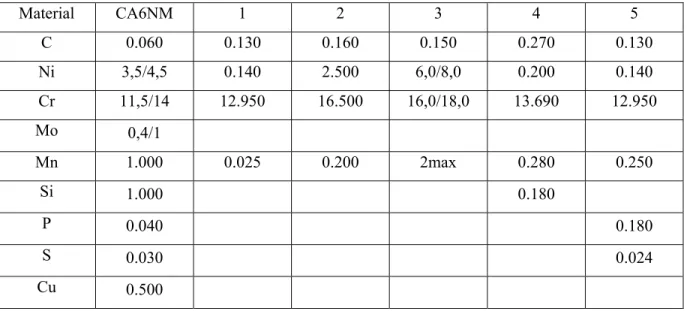
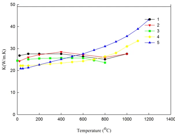
Specific heat is a temperature dependent property, defined as the amount of heat needed to raise the temperature of a certain quantity of material [32]. A comprehensive literature review revealed that the specific heat values were not reported for stainless steel 415 [33-35]. A reasonable approach to tackle this issue could be to use the specific heat of similar materials [27]. Therefore, the specific heats of five steels that have similar chemical compositions were collected and then interpolated to approximate the specific heat of stainless steel 415. The compositions of five similar materials are presented in Table 1.1.
Table 1.1 Chemical compositions of CA6NM and five similar materials Material CA6NM 1 2 3 4 5 C 0.060 0.130 0.160 0.150 0.270 0.130 Ni 3,5/4,5 0.140 2.500 6,0/8,0 0.200 0.140 Cr 11,5/14 12.950 16.500 16,0/18,0 13.690 12.950 Mo 0,4/1 Mn 1.000 0.025 0.200 2max 0.280 0.250 Si 1.000 0.180 P 0.040 0.180 S 0.030 0.024 Cu 0.500
Specific heat values of the mentioned materials versus temperature are plotted in Figure 1.6. As it can be observed, phase transformation of martensite → austenite in stainless steel can affect the specific heat in a temperature range of 600℃ to 800℃, whereas, the literature did not provide comprehensive information about the amount of heat specific for this phase transformation. Furthermore, the literature only provides data for increasing of the temperature. No information can be found for the austenitized material before developing of the martensite during the cooling. Therefore, further experimental investigations are needed to measure specific heat of stainless steel 415. The solid-state phase transformation was not observed within the DSC thermograph of material # 1 to 3 due to the absence of the exothermic. However, as it is shown in Figure 1.6, specific heat of material # 4 and 5 exhibited a change during the phase transformation. In this study, specific heat was measured distinctly during heating and cooling. This is discussed in section 4.5.
Figure 1.6 Specific heat vs. temperature for five different materials during heating
1.3.4.2 Thermal conductivity
Thermal conductivity is a material property characterizing the ability of material to conduct heat. Thermal conductivities of the materials in Table 1.1 are presented in Figure 1.7.
Figure 1.7 Thermal conductivity vs. temperature for five different materials
1.3.4.3 Convective heat transfer
Convective heat transfer coefficient is not a material property. Here, convection occurs between the metal surface and environment owing to the molecular mobility of the surrounding air. The convective heat transfer is estimated using equation (1.4) [29, 32].
= ℎ( − ) (1.4)
Where q, h, T and Ts stand for heat flux ( ⁄ ), convection heat transfer coefficient ( ⁄ ℃), material temperature (°C) and ambient temperature, respectively. The convective heat transfer coefficient, h, is considered to be 8 ( ⁄ ℃) according to the experimental work carried out at IREQ [36].
1.3.4.4 Radiation heat transfer
Radiation is the energy transported at the speed of light in the absence of material. Radiation depends on the forth power of the absolute temperature[37]. The contribution of the radiation heat transfer is assumed noticeable at high temperatures (1.5).
= . . ( − ) (1.5)
Where q, σ, ℰ, T and stand for heat flux ( ⁄ ), Stefan-Boltzmann constant (5.67 − 8 ⁄ ), emissivity, material temperature (K) and ambient temperature (K).
Here, emissivity depends on surface oxidation and temperature variations [32]. The emissivity of steel 415 is presented in Figure 1.8.
Figure 1.8 Variation of emissivity coefficient for stainless steel 415 as a function of maximum temperature
1.4 Heat source models
The input heat from welding causes a complex thermal cycle in the weldment. Subsequently, thermal stresses and microstructural variations result in the residual stress and distortion of the final product [7]. Residual stress and microstructural changes are predicted based on the welding thermal cycle. Moreover, the predicted thermal cycle provides information on the geometry of the heat-affected zone, the cooling rate as well as the weld penetration [38]. It has been demonstrated that a deep understanding of the thermal cycle is strongly required, particularly in a region nearby the heat source. Consequently, an accurate heat source model is needed in order to predict the exact temperature distributions [39]. To date, various methods have been developed to predict a thermal cycle precisely.
1.4.1 Rosenthal’s analytical model
Rosenthal developed a mathematical theory of heat distribution using the conventional heat transfer differential equation. He presented a method for predicting cooling time and its rate in welding Rosenthal’s analysis [40]. This method exhibited an analytical solution for the temperature distribution considering the heat source as a point, line, or plane [39]. Rosenthal’s method is still the most popular analytical method to evaluate the thermal history of welds [41].
Rosenthal’s theory was the first mathematical theory, capable of predicting the heat distribution of a moving heat source [42], However it was derived from a single formula [40]. For the first time, Rosenthal solution makes it possible to consider welding parameters such as current, voltage and welding speed in the analysis [31, 43]. Equation (1.6) presents Rosenthal’s equation for temperature distribution around the moving sources of a two dimensional problem [44, 45].
( − ) = 2
Where, T, , Q, K, α, V, R and W stand for temperature at a point (K), original plate temperature (K), heat input per unit time (W), thermal conductivity ( . . ), thermal diffusity ( . ), welding speed ( . ), distance to heat source (m) and distance along the weld center line (m), respectively.
Temperature field is predicted accurately far from the heat source using either point heat source, line heat source or surface heat source. However, this solution cannot predict temperature in or in the vicinity of fusion zone (FZ) and heat affected zone (HAZ). Furthermore, it is not either suitable for complex welding assemblies. This is a major drawback of this method, since this approach could not consider temperature-dependent properties of material as well as real boundary condition. Furthermore, the flux and temperature at the heat source have been assumed infinite in this model. These assumptions lead to considerable errors in estimation of temperature in comparison with experiments. In addition, Rosenthal’s solution provides no information related to the weld pool [6, 39, 42-44, 46-50].
1.4.2 Numerical methods
Inherent assumptions made to derive the equations are known as a limitation of analytical approaches. Numerical models have been developed to overcome the limitations of analytical methods. Finite element methods (FEM) is among the most widely used numerical methods. The FEM can manage analyses of complex geometries and temperature dependant material properties [24].
Rykalin [51] applied Fourier’s heat flow theory to a moving heat source to solve one and two dimensional heat flow problems using a numerical method [49]. The long running time had restricted the application of this model. Furthermore, either limited number of elements or coarse elements have been considered to overcome this drawback. This may sacrifice the accuracy of prediction in 1951 (cited by [43, 45]).
Westby prevailed the restriction of elements size and number as well as constant thermal properties by high performance computer in 1968 [43, 45].
Paley presented a computer program based on Westby work capable of analyzing non-rectangular cross sections such as V and U grooves using a non-uniform mesh.
Paley and Hibbert [43] and Westby [52] assumed that energy was distributed with a constant power density throughout the melted zone to reflect the digging effect of the arc with a finite difference analyses [6, 46, 47, 49, 53-55]. In 1975, Paley and Hibbert published a paper in which they described their model taking variable thermal properties into account and predicting actual weld shape and thermal history of the welding process [43]. However, in 1984 Goldak et al. demonstrated that this model was not able to predict complex geometry of welding pool because of using finite difference analyses. Furthermore, it did not present any criteria to predict the length of molten pool [6, 46, 49].
1.4.2.1 Disc model
Gaussian distribution of flux deposited on the surface of the work piece was proposed by Pavelic [56] for the first time. This distribution is described by equation (1.7).
( ) = (1.7)
Where ( ), q0, C and r stand for the surface flux at radius r (W/ ), the maximum flux at the center of the heat source (W/ ), the distribution width coefficient ( ) and the radial distance from the center of the heat source (m), respectively.
In disc model, the input energy is considered as the total energy of arc (Q). The uniform flux and C can be correlated where, is distributed in a circular disk, of diameter = 2
= 4
(1.8)
= (1.9)
( ) = (1.10)
C is related to the width of the heat source. Therefore, a more concentrated source such as laser beam shows a smaller diameter d and a larger C. Variation of C is shown in Figure 1.9. In order to measure the value of C, it is assumed that the imposed heat flux in the circle with radius( ) is equal to 5% of the maximum heat flux at the center of heat source.
( ) = (1.11)
0.05 = (1.12)
= (20)≈ 3 (1.13)
Pavelic’s distributed heat source model was explored by Krutz [1]. He applied a two dimensional finite element analysis to determine a relationship between temperature and time. He considered thermal conductivity and specific heat as a function of temperature and assumed a Gaussian distribution for heat flux.
It has been shown that the heat source model derived by Pavelic [56] and Krutz [1] can represent a precise prediction of temperature distribution. However, the arc penetration is as small as GTA welding since the contribution of arc digging action has been neglected in this model [6]. Thus, it increases the errors related to high power density sources, such as laser beam or electron beam.
Eagar and Tsai [44] presented a dimensionless solution for a traveling Gaussian distributed heat source in 1983. The same simplifications as Rosenthal’s theory were assumed such as
constant thermal properties and quasi-steady state semi-infinite. Eagar and Tsai successfully provided a first estimation of weld pool geometry based on fundamentals of heat transfer [39, 44]. Literally, this model demonstrated an accurate functional relation between both process and material parameters. Nonetheless, it cannot predict weld penetration accurately. Eagar and Tsai proposed to employ Myers [57] temperature enhancement factor to obtain better results.
Figure 1.9 Schematic of disc model Taken from Pavelic (1969)[56]
1.4.2.2 Hemispherical power density distribution
As it was described earlier in 1.4.2.1, disc model is not an appropriate approach for the heat source with a high power density since the arc transports the heat under the surface. Hemispherical Gaussian distribution of power density has been suggested as a more realistic model for these types of heat sources. Hemispherical distribution is determined by equation (1.14) [46].
( , , ) = 6√3 √
(1.14)
Where q, C and c stand for power density ( ⁄ ), distribution width coefficient ( ) and the radius of hemispher ( ), respectively.
As a matter of fact, hemispherical heat source solves the problem of ignoring the arc penetration. Nevertheless, it shows some limitations in modeling of a heat source. It assumes heat source embedded in a spherical symmetry. Ellipsoidal volume source is proposed to figure out this limitation.
1.4.2.3 Double-ellipsoidal Model
All the aforementioned methods suffer from several serious restrictions. Goldak [6] initially proposed a semi-ellipsoidal heat source with Gaussian heat flux distribution. This model is more precise allowing controlling the arc penetration. Heat Gaussian distribution is determined inside the volume by the equation (1.15)
( , , ) = (1.15)
Where is maximum value of the power density at the center of ellipsoid and A, B and C are heat flow distribution coefficients.
The energy of arc is equal to the heat flux Q since heat flow is distributed inside the semi-ellipsoid volume. Heat flux is calculated by multiplying the voltage and current by a coefficient of 2. The coefficient is related to the overall applied energy in a half ellipsoid. Q is calculated as follow: 2 = 2ɳ = 8 ( , , ) = 8 ( √ 2√ )( √ 2√ )( √ 2√ ) (1.16)
In the equation (1.16), η, V and I represent heat source efficiency, the voltage of the arc and current of the arc, respectively.
=2 √ √
(1.17)
It is speculated that power density on the surface of the ellipsoid with the spreading parameter of arc (a, b, c) is 0.05q0 [46]. So:
= 3 , = 3 , = 3
The experimental findings showed that the ellipsoid model could not precisely predict temperature gradient in front of the heat source. Double ellipsoidal source is suggested to overcome this limitation. The front half of the source is the quadrant of one ellipsoidal source, and the rear half is the quadrant of another ellipsoid. In this model, and are the rear fraction and front fraction of heat respectively, deposited in the front and rear quadrants, where + = 2. The power density distribution inside the front quadrant is:
( , , , ) =6√3
√ ∗ ∗
( ( ) (1.18)
The power density distribution is calculated in the rear quadrant similar to the front quadrant.
( , , , ) = 6√3
√ ∗ ∗
Figure 1.10 Double ellipsoid heat source
configuration Taken from Goldak (1984) [6]
Recently, a research has been carried out on thermal analysis of the heat source. Lundbäck [58] suggested to combine conical heat source and ellipsoid heat source. This model is consistent for a welding with high penetration such as electron beam welding. This model can accurately predict the penetration, as it was demonstrated by the comparison of finite element results with the experiments. Nevertheless, full penetration has not been achieved in the finite element model. Hong proposed a combination of body heat power and surface heat flux [23] for modeling of gas metal arc welding. It is mentioned as a simple model for asymmetric multi pass welding. Hong’s model has also been used for modeling of gas metal arc welding. The ratio of surface heat flux and body heat flux has been adjusted to achieve an accurate representation of fusion zone. In Hong’s study [23], surface heat flux was assumed to be in the form of Gaussian thermal distribution while the body heat flux was assumed to be constant.
A split heat source has been suggested by Wahab [38] to consider the heat transfer through convective movement of the liquid weld pool. This fact was neglected in Goldak model. Wahab [38] developed two conduction models as a 2D model and a 3D finite element model. In his approach, the total heat is split into several parts and distributed. One part of the heat input arises from the inclusion of a deposited weld bead. Then, the remaining heat is divided
into arc and drop sources. The part related to the arc is an ellipsoidal volume at the plate surface. The second part, from the drop is distributed below the plate surface at a depth proportional to the arc current. The result illustrates that the simple 2-section model and the 3D finite element conductive heat transfer models adequately simulate the gas metal arc welding.
In another study, Ohm divided the weld bead into N parts and sequentially deposited in time [59]. In this finite element analyses, the elements of weld bead have been activated at a specific time point, and then material properties and temperature were changed to bead material values. A constant temperature ( ) is applied to all nodes. Thermal analysis is solved for the first weld bead then the temperature load is removed from the first weld bead. In final step, same process is frequently run for each N in a weld bead. This numerical model is used for a single bead weld on a steel plate. This approach revealed better results on prediction of residual stresses compared to the moving heat source while moving heat source can estimate the temperature distribution more precisely. However, the estimation of residual stress is strongly interconnected to the prediction of the temperature distribution. In other words, more precise temperature distribution is calculated, the more accurate residual stress.
1.5 Stainless steel 415
The application of chromium steel is limited, owing to the brittleness of precipitated chromium carbide at the grain boundaries during welding, poor weld ability and consequently its cold cracking sensitivity [60].
Stainless steel 415 is a modified chromium steel via the reduction of the percentage of carbon and the addition of 3-4 % Ni to improve corrosion resistance and toughness [60, 61]. Therefore, 13 % Cr and 4 %Ni are distinguished in stainless steel 415 to improve its resistance to corrosion, cavitation corrosion, excellent weld ability and high strength [17, 62, 63]. Manufacturing of hydraulic turbine is one application of this stainless steel [17, 61, 64].
Weldability is an important feature of stainless steel 415. Nonetheless, a crack-free weld is acquired in thick plate using a matched filler metal (12% Cr, 4-6% Ni) and preheating [60].
Delta ferrite forms during solidification of stainless steel 415 according to the phase diagram as it is presented in Figure 1.11. The phase transformation of delta ferrite to austenite occurs in a temperature range of 1200˚C-1300 ˚C. Subsequently, austenite (f.c.c) transformed into martensite (b.c.c) during the cooling step with a volumetric change. However, the final structure of stainless steel can contain delta ferrite in a range of 1-4 %.
The combination of strength and toughness is optimized through austenitizing and tempering of stainless steel [65]. Toughness increases by tempering heat treatment in a range of 600℃ -620℃ accompanied with a decrease in the hardness of this material [60]. The microstructure of stainless steel is lath martensite after austenitizing. The variation of the volume fraction of the reformed austenite formation can occur in the tempering temperature range of 570℃-680℃ using different holding times. The formation of reformed austenite only depends on temperature as the tempering temperature reaches 680℃ [65].
Reformed austenite is distributed inter lath boundaries along the martensite. Accordingly,
high toughness of stainless steel after tempering is due to distribution of reformed austenite. Reformed austenite causes softening through transformation to martensite near crack. Transformation of austenite (fcc) into martensite (bcc) absorbs energy and closes cracks by volume expansion resulted from phase transformation. Therefore, reformed austenite is thermally stable but not mechanically. Nevertheless, austenite transforms into martensite at even a low stress [17, 62, 66]
The reformed austenite is stable as it cools down to room temperature from the tempering temperature between 600℃-630℃. However, the reformed austenite produced in a tempering temperature above 630℃ is partially transformed to martensite during cooling [67]. It has been shown that the reformed austenite is enriched with Ni atoms and the segregation of Ni makes reformed austenite stable. An increase of temperature improves amount of reformed
austenite decreasing the concentration of Ni [65]. It makes the reformed austenite less stable due to diminution amount of Ni atom [62].
Figure 1.11 Phase diagram of stainless steel 415 Taken from Folkhard (1988) [68]
1.6 Summary
In this chapter, a comprehensive literature review is carried out on base material’s properties and different moving heat source models. This review would broaden our understanding of welding process and would help us to calculate the thermal field for multi-pass welding accurate.
CHAPTER 2
RESEARCH OBJECTIVES AND HYPOTHESIS
Welding is a useful industrial process in turbine manufacturing and shipbuilding. As the arc crosses the weld assembly, residual stresses are produced because of the very steep thermal gradient and subsequent phase transformation. A precise modeling of the welding can predict welding outcome without requiring costly pre-production. Furthermore, it provides a comprehensive understanding of the welding process [38]
Finite element method has shown promising results in the modeling of welding as it can be seen in the numerous published studies [21, 27]. Among different approaches, most studies used Goldak’s moving heat source model to simulate temperature gradient. Moreover, element birth and death method has been suggested to consider deposition of filler metal in simulations.
After reviewing the literature relevant to the stainless steel 415, it is recognized that there is a lack of knowledge about thermal properties of this material such as specific heat and conductivity coefficient in different temperatures. Improvements in the understanding of the aforementioned material properties would lead to a significant contribution into simulation of welding process. Furthermore, a FEM which is able to predict the temperature contour with time within or nearby the heat affected zone is of high interest.
The global objective of this research is to accurately calculate the thermal field within and in the vicinity of the heat affected zone for multi-pass flux cored arc welding of stainless steel 415.
This study presents a three passes 410Nimo FCAW welding, performed on a triangular groove made on a AISI415 plate. Simulations were carried out using the thermal finite element code developed at IREQ to calculate the thermal field for multi-pass welding.
The research hypotheses of this thesis are:
• Temperature variations with time can be predicted within the heat-affected zone during a multi-pass welding process, using the developed FEM, with an average envisaged error less than 10% for the maximum temperature.
• Thermal conductivity and specific heat are considered as a function of temperature and a Gaussian distributed heat flux is used to determine temperature time relationships in this research.
To address the main objective, three specific objectives are defined:
Objective 1: To measure the specific heat and conductivity coefficients for stainless steel 415 by an experimental set up
Objective 2: To validate calculated thermal distributions during multi-pass welding through experimental investigation
Objective 3: To validate the finite element model by comparing the microstructure in small samples after applying the resultant thermal history from simulations with the experimental results.
CHAPTER 3
METHODOLOGY AND EXPERIMENTAL CHARACTERIZATION 3.1 Introduction
The purpose of this thesis is to develop a model to precisely predict the temperature profile nearby a heat source such as a welding zone. In order to validate the calculated results, temperature profiles were recorded through thermo-couples installed at different locations of a plate, during a multi-pass welding process. Furthermore, heat-affected zones (HAZ) were investigated using micro hardness measurements and micro-structural analysis of the plate cross section. Finally, experimental reproduction of thermal profile estimated at some nodes of the welded plate FEM model was carried out on base material samples, and micro hardness of these samples were compared to that of the actual welded plate at the same location. In this section, the characteristics of the installation, instrumentation and welding process are described.
Figure 3.1 Experimental strategy 3.2 Base material
Heat treatment was required in order to prepare the plate for welding process as the first step of the experimental procedure. Initially, the property of the base material should be
Plate of martensitic stainless steel 415
Welding Installing 20 K-type
thermocouples
Machining Heat treatment Installing 5 K-type
investigated. Martensitic stainless steel 13%Cr–4% Ni was employed as the base material in this study. This type of stainless steel contains Chromium, Nickel and a low percentage of Carbon. Furthermore, It is well-known for the high weld quality, high mechanical strength, and excellent corrosion resistance [17] as described in 1.5. The chemical composition of the base material and filler metal are presented in Table 3.1.
Table 3.1 Chemical composition of the base material and filler metal(wt%)
% C % S % P % Si % Mn % Cr % Ni % Mo % V % Cu Base
metal 0.017 0.001 0.015 0.47 0.8 12.0 4.2 0.58 0.02 0.17
Filler
metal 0.02 0.005 0.01 0.38 0.4 12.4 3.9 0.52 0.02 0.05
The term “Martensitic” is designated to the base metal since the microstructure is mainly included martensite. Austenite, martensite and α-ferrite are the main components of martensitic stainless steel. The amount of austenite and martensite depends on the applied heat treatment. Moreover, the amount of α-ferrite was detected to be up to 5 vol % in the base material [17, 64].
3.3 Heat treatment
Heat treatment consists of heating a metal to a specific temperature, holding it at that temperature for a required time, and finally cooling it to ambient temperature [69]. Heat treatment has been recommended to optimise physical and mechanical properties of the materials and to obtain a desired metallurgical structure [70]. The structure of a metal can be influenced by maximum temperature, holding time, rate of cooling and heating [69]. Ultimate structure of a metal can be predicted by its phase diagram [70]. Annealing, normalizing, aging, stress relieving, quenching and tempering are different types of heat treatment. One of the most important applications of the heat treatment process is to soften and reduce the hardening and to increase the toughness as it is employed in this study.
Various temperatures and holding times were selected to heat treat small specimens of base material. Hardness measurement and microstructure analysis were performed to achieve minimum hardness in the absence of grain growth. The key aspect of using heat treatment was to reduce as much as possible the hardness of the base material in order to produce the largest range of microhardness in the heat affected zone of the welded plate. That would increase the resolution of the hardness map since the hardness would remain low in the base metal far from the weld and very high in the weld metal and HAZ, since austenization and martensitic transformation is attended to occur. Heat treatment steps to achieve this lowest hardness of the base metal are described in section 3.4 with more details.
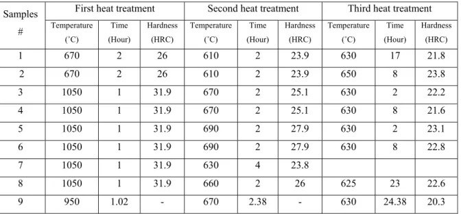
3.4 Heat treatment steps
The hardness for the base material (prior to the heat treatment) was measured to be 26 HRC, respectively. This as-received condition from the steel supplier Carlson was achieved by austenitizing at 1050°C, followed by a double tempering heat treatment.
Samples, from the base metal, were prepared with a square cross section (38.1×38.1 mm2) and a height of 76.2 mm. These were subjected to various heat treatment procedures.
The samples were put in a furnace and held for a sufficient period at a desired temperature. Subsequently, the samples were taken out and cooled rapidly to room temperature.
Heat treatment sequences and resulting hardness are presented in Table 3.2. After each step, hardness of the heat-treated samples were measured with a load of 150 kg on the Rockwell-C scale.
Heat treatments for samples #1 and #2 were triple tempering heat treatments added to the previous double-tempering given by the supplier at similar temperatures. As expected, the amount of reformed austenite has probably increased since the hardness reduced from 28.3 HRC to 21.8 HRC (WP #1).
The purpose of heat treatments for samples #3 to #8 was to re-austenitize the steel, therefore completely removing the initial Carlson metallurgical condition (which was unknown to us) and impose our own double-tempering heat treatment directly from the as-quenched condition. The selected heat treatment (last line of the table) was a re-austenitizing at a slightly lower temperature (because the capacity of the available furnace to hold the whole plate could not exceed 1000°C), with a 24 h sustained second tempering heat treatment at 630°C. An average hardness of 20.1 HRC +/- 1.2 was obtained out of 10 measurements on the plate.
Table 3.2 Summary of heat treatment temperature, time and hardness for different tests
The plate was made of martensitic stainless steel 13%Cr-4%Ni with length, width and thickness of 472 ×254×38.1 mm3 respectively.
As discussed in the last section, the plate was heat treated in a three-step sequence, as described below
In the first step, the plate was held in the oven at 950 ℃ for 1.03h in order to austenitize the plate in depth. The set point of the furnace was adjusted to obtain 950°C as the average response of five K-type thermocouples tack welded on the plate, as indicated in Figure 3.2.
Samples #
First heat treatment Second heat treatment Third heat treatment Temperature (˚C) Time (Hour) Hardness (HRC) Temperature (˚C) Time (Hour) Hardness (HRC) Temperature (˚C) Time (Hour) Hardness (HRC) 1 670 2 26 610 2 23.9 630 17 21.8 2 670 2 26 610 2 23.9 650 8 23.8 3 1050 1 31.9 670 2 25.1 630 2 22.2 4 1050 1 31.9 670 2 25.1 630 8 21.6 5 1050 1 31.9 690 2 27.9 630 2 23.1 6 1050 1 31.9 690 2 27.9 630 8 22.8 7 1050 1 31.9 630 4 23.8 8 1050 1 31.9 660 2 26 625 23 22.6 9 950 1.02 - 670 2.38 - 630 24.38 20.3
Figure 3.2 Installation of five k-type thermocouples to control the temperature
inside oven during heat treatments (This picture was taken after a first heat treatment, where the plate was
rapidly cooled. The plate was reheated and slowly cooled in the furnace)
This temperature was maintained for 1.03 h. The plate was then slowly cooled down in the furnace. Phase transformation within the steps was predicted from equilibrium diagram of stainless steel 13%Cr-4%Ni.
Austenitization occurred in the plate at 950℃ according to phase diagram (Figure 1.11 ). The austenite to martensite (γ → M) phase transformation took place as the plate was being cooled down. Consequently, the microstructure of base material was transformed entirely into fresh martensite as it was described in chapter 1 [18, 66].
In the second step, the plate was held at 670°C for 2.38 h, subsequently being cooled down to room temperature. The microstructure then consists of a mixture of austenite and martensite at room temperature after tempering at 670℃. According to the phase diagram, austenite appears in the microstructure at a rough temperature range of 620 ℃ to 720℃.
Consequently, fresh martensite was converted to a tempered martensite and reformed austenite at this stage. It is consistent with the micro hardness measurements as the measured value for hardness decreased to 25.1 HRC.
The third step included holding the plate at 630°C for 24 h, then cooling it down to room temperature. The ultimate microstructure of the base material was tempered martensite and more reformed austenite compared to the second step. The plate hardness was measured to be 20.3 HRC.
No grain growth was confirmed by microstructural investigations using optical microscopy. Figure 3.3 revealed no grain growth occurred during the heat treatment of sample 9. Figure 3.3-a and Figure 3.3-b indicated the microstructure of martensitic stainless steel prior to the heat treatment and after 3-step of heat treatment, respectively. The micrograph exhibited that the grain size was the same for both samples.
Figure 3.3 The microstructure of martensitic stainless steel a) before heat treatment
b) after heat treatment
3.5 Preparation of plate and V-groove
In this process, the heat-treated plate was ground to its final shape and size. The V groove preparation has been suggested for welding of thick plates similar to the one employed in this study [2].
Schematic picture of the plate and v-groove is presented in Figure 3.4. The z-axis designated to the longitudinal direction of the plate. The x and y-axes were assigned to the transverse and normal directions, respectively. V–groove was prepared along the z direction for multi-pass welding.
Figure 3.4 Schematic picture of machined plate and V-groove
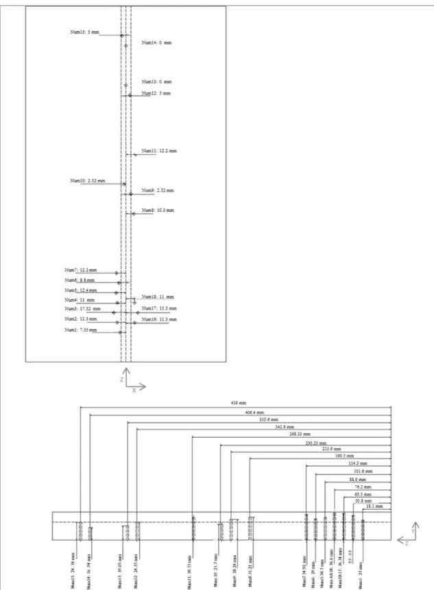
Moreover, eighteen 3.26 mm diameter holes were drilled in the inferior surface of the plate to embed thermocouples. As shown in Figure 3.5, these holes were located in the x-z plane at different depth.
Y X
Figure 3.5 Schematic picture of v-preparation and drilled holes
The locations of thermocouples were determined through simulations. Critical temperatures for base material specimens were set within a temperature range between 620℃ and 720℃ corresponding to the phase transformation (M→ γ) occuring in the base metal. Consequently, it is expected that the microstructure and hardness of base material will change in HAZ. The 18 thermocouples were installed in the processed holes, in the lower face of the plate. Furthermore, two more thermocouples were installed on the upper surface of the plate to monitor temperature far from the welding zone.
Figure 3.6 Drawing for machining, indicating the position of thermocouples on the plate
3.6 Thermocouples installation
The thermal history induced by welding was recorded experimentally. K-type thermocouples were employed in this research. Schematic set up of K-type thermocouples is presented in Figure 3.7. This type of thermocouples consists of two different wires protected against a contact with the plate by a ceramic tube with two holes. Each wire is passed through a hole in ceramic tube [27]. It is worth noticing that the k-type thermocouples are limited to applications with the temperature lower than 1200℃. The positions and depth of thermocouples are shown in Figure 3.5.
Figure 3.7 Schematic picture of K-thermocouples & installation 3.7 Characteristic of the welding set up
Flux-cored arc welding (FCAW) was employed as the welding process in this study. The base material and the filler metal were martensitic stainless steel 415 and 410 Ni-Mo TQS 1/16, respectively. The filler metal and the base metal have similar chemical compositions illustrated in Table 3.1. The plate was simply supported at three points to minimize heat transfer by conduction through direct contact with the structure. The installation of plate and welding torch are presented in Figure 3.8.
Figure 3.8 Installation of the plate on three points
Multi-pass welding was required to fill the V-groove in this study. Multi-pass welding is suggested to weld thick plates to avoid high current and to maintain adequate properties in the HAZ.
Prior to the first pass, the plate was preheated to 100℃ to ensure crack free welding [60]. The first pass was positioned at x=127 mm, = 25.4 mm, and z varying from 0 to 457.2 mm. The arc characteristics were voltage of 28V, current of 292.9A, and feed rate of 6.5mm/s. A backhand technique was conducted for the three passes accompanied by a travel angle of
6˚.1 A work angle of 90˚ was applied for the first pass. In addition, the molten weld pool and hot surrounding metal were protected from ambient air for the three passes by mixed gas Argon- 25% .
Figure 3.9 Schematic picture of coordinates and work angle of first pass
The second pass of welding was positioned at x=123.698 mm, y=32.512 mm and z varying from 0 to 304.8 mm. Inter pass temperature was approximately 150 ℃ for the second pass. A work angle of 65˚ was applied for second pass as shown in Figure 3.10. The arc characteristics were voltage of 28 V, current of 292.9 A, and feed rate of 6.5 mm/s.
1 In the backhand welding technique, the torch is held perpendicular to the plate, tilting in the direction of welding for 6 degrees.
Figure 3.10 Schematic picture of coordinates and work angle of second pass
The angle between torch and the plate (work angle) for the second welding is presented in.Figure 3.11.
Figure 3.11 Installation of the plate and angle of torch for second pass of welding
The third pass of welding was positioned at x= 129.54 mm, y=32.512 mm and z varying from 0 to 152.4 mm. The inter pass temperature was measured to be 150℃. Arc characteristics were voltage of 28 V, current of 294.3 A, and feed rate of 6.5 mm/s. A work angle of 90˚ was applied for third pass too.
Figure 3.12 Schematic picture of coordinates and work angle of third pass
3.8 Microstructure analysis
The fully reversible nature of the phase transformation (γ →M) is known as an exceptional feature of martensitic steel 13%Cr- 4%Ni. The fraction of austenite transformed in the HAZ depends on the thermal cycle at each point. The measured hardness in HAZ reflects the fraction of martensite transformed to austenite.