Bouakez : HEC Montréal and CIRPÉE. Correspondence : HEC Montréal, 3000 Côte-Sainte-Catherine, Montréal,
QC, Canada H3T 2A7. Tel. : 1 514 340-7003; Fax : 1 514 340-6469 [email protected]
Chihi : HEC Montréal and CIRPÉE Normandin : HEC Montréal and CIRPÉE
Cahier de recherche/Working Paper 11-23
Fiscal Policy and External Adjustment: New Evidence
Hafedh Bouakez
Foued Chihi
Michel Normandin
Abstract:
Relatively little empirical evidence exists about countries’ external adjustment to
changes in fiscal policy and, in particular, to changes in taxes. This paper addresses this
question by measuring the effects of tax and government spending shocks on the
current account and the real exchange rate in a sample of four industrialized countries.
Our analysis is based on a structural vector autoregression in which the interaction of
fiscal variables and macroeconomic aggregates is left unrestricted. Identification is
instead achieved by exploiting the heteroscedasticity of the structural disturbances.
Three main findings emerge: (i) the data provide little support for the twin-deficit
hypothesis, (ii) the estimated effects of unexpected tax cuts are generally inconsistent
with the predictions of standard economic models, except for the US, and (iii) the
puzzling real depreciation triggered by an expansionary public spending shock is
substantially larger in magnitude than predicted by traditional identification approaches.
Keywords: Government spending, current account, exchange rate, taxes, structural
vector auto-regression, twin deficits
1.
Introduction
The latest financial crisis has revived interest in the macroeconomic effects of fiscal policy and its role as a stabilization tool, as nominal interest rates approached zero, leaving little room for monetary policy. However, while a large body of work has focused on assessing the effectiveness of tax and public spending policies in stimulating output and domestic absorption, relatively less effort has been devoted to studying the implications of those policies for countries’ external adjustment and, by extension, for global imbalances. In particular, to our knowledge, only one paper, namely Kim and Roubini (2008), attempted to empirically evaluate the reaction of the current account and the real exchange rate to changes in taxes, and only a handful of studies attempted to measure the response of those two variables to changes in government spending (Corsetti and M¨uller 2006; Kim and Roubini 2008; M¨uller 2008; Monacelli and Perotti 2010; Enders, M¨uller and Scholl 2011). This is somewhat surprising given that the current account is commonly regarded as a barometer of a country’s solvency, and that exchange-rate fluctuations critically affect a country’s competitiveness on the world market and its trade balance.
Using structural vector autoregressions (SVARs) and focusing mostly on US data, the papers cited above find that unexpected tax cuts and increases in public spending unambiguously depre-ciate the real exchange rate. Kim and Roubini (2008) also find that a surprise tax cut worsens the budget deficit but improves the current account, a situation referred to as “twin divergence”. On the other hand, no consensus has been reached regarding the effects of an unexpected increase in government spending on the current account, or whether it leads to twin divergence or twin deficits (i.e., positive comovement between the budget and external deficits).
Generally speaking, these findings are puzzling from a theoretical standpoint. A wide class of open-economy macro models indeed predict that an unexpected fiscal expansion should appreciate the currency in real terms and deteriorate the current account. In the case of a tax cut, the real appreciation occurs because there is a higher incentive to invest,1 which raises the real interest rate. The rise in investment is typically larger than the increase in national saving, causing a
current-1
account deficit. In the case of an increase in government spending, the appreciation results from the fact that public expenditures are relatively more intensive in domestically produced goods, which means that the increase in aggregate demand brought about by the increase in public spending will raise their relative price with respect to foreign goods. The rise in public spending also entails a negative wealth effect that induces households to borrow abroad to prevent a large drop in their consumption, thus worsening the current account.
The purpose of this paper is to provide new evidence on the effects of fiscal policy on changes in the net foreign position and on the real exchange rate in a sample of four industrialized countries, namely, Australia, Canada, the United Kingdom, and the United States. These four countries are known to have reliable non-interpolated quarterly data on fiscal variables. Our contribution to the empirical literature is threefold. First, we provide more comprehensive evidence on the response of the current account and the exchange rate to changes in taxes than Kim and Roubini, who focused exclusively on the US. Second, we use an estimation strategy that relaxes the identifying assumptions used in previous SVAR-based studies, which restrict the interaction of the variables of interest in a rather arbitrary way. Third, we document the implications of imposing these restrictions for the response of the current account and the exchange rate to fiscal shocks.
Our empirical strategy builds on that developed in our earlier work (Bouakez, Chihi, and Normandin 2010). More specifically, we identify fiscal-policy shocks by exploiting the conditional hetereoscedasticity of the shocks. When there is enough time variation in the conditional variances of the time series used in estimation, it becomes possible to identify the structural shocks and their effects without having to impose additional parametric restrictions, as would be the case under (the usually maintained assumption of) conditional homoscedasticity (see Sentana and Fiorentini 2001). Incidentally, several studies document that the macroeconomic time series that we use in our analysis display significant time-varying conditional volatilities.2 In our framework, the matrix of contemporaneous interaction nests the parametric restrictions typically imposed in the literature,
2
See, for example, Hsieh (1988, 1989), Engel and Hamilton (1990), Garcia and Perron (1996), Den Haan and Spear (1998), Engel and Kim (1999), Fountas and Karanasos (2007), Fernandez-Villaverde, Guerr´on-Quintana, Kuester, and Rubio-Ram´ırez (2010), and Fernandez-Villaverde, Guerr´on-Quintana, Rubio-Ram´ırez, and Uribe (2011).
thereby allowing one to assess the bias resulting from such restrictions.3
The empirical framework developed in our earlier paper casts fiscal policy in the context of a market for newly issued government bonds. The supply of bonds may or may not shift as a result of changes in taxes or public expenditures, depending on the government’s implicit target. In turn, variations in taxes and public expenditures reflect both the automatic and systematic responses of these variables to changes in economic conditions, as well as fiscal-policy shocks. We extend this framework by assuming that the demand for government bonds originates not only domestically but also abroad, implying that the real exchange rate enters the bond-demand equation. We also include the current account among the vector used in estimation, while leaving its interaction with the remaining variables completely unrestricted.
Our results show important differences in the response of the current account to tax shocks across the four countries. While the current account remains essentially unresponsive to unex-pected tax cuts in Australia and the UK, it improves in Canada and deteriorates in the US. In contrast, the primary budget deficit worsens in all cases, implying that the twin-deficit hypothesis (conditional on a tax shock) is supported only by US data. We also find that the real exchange rate remains essentially unchanged following the tax cut in Australia and the UK, but that it appre-ciates significantly and persistently in Canada and the US. These findings are novel and have not been previously reported in the empirical literature. Importantly, they are generally at odds with the predictions of standard economic models, except in the US. Finally, we show that imposing the restrictions commonly used to identify tax shocks leads to important mis-measurements of their effects. For example, the identification schemes proposed by Kim and Roubini (2008) or Monacelli and Perotti (2010) counterfactually imply that unexpected tax cuts lead to a twin divergence and to a real depreciation in the US.
3
Leeper, Walker and Yang (2008) pointed out that the SVAR approach may not be robust to fiscal forsight– the phenomenon that, due to legislative and implementation lags, economic agents are likely to react to changes in taxes and governement spending several months before those changes actually take place. In the extreme case where all fiscal shocks are anticipated, Leeper et al. show that the resulting time series may have a non-invertible moving average component, such that it would be impossible to recover the true fiscal shocks from current and past variables. In, Bouakez, Chihi, and Normandin (2010), however, we provide suggestive evidence that the fiscal foresight problem is not sufficiently severe to undermine the SVAR approach. This is likely due to the fact that empirical studies mostly use quarterly data and that an important fraction of the changes in fiscal policy are implemented within a quarter,
Regarding the effects of government spending shocks, our results also reveal the absence of a clear pattern regarding the reaction of the current account. In response to an unexpected increase in public spending, the current account deteriorates in the UK, improves with a delay in Canada and the US, and remains unchanged in Australia. For its part, the budget deficit shrinks with a delay in Australia and the UK and worsens in Canada and the US. Again, these findings lend little support to the twin-deficit hypothesis. As for the real exchange rate, it depreciates significantly in all countries, except Canada, where it exhibits a muted and statistically insignificant response. Interestingly, our results indicate that the magnitude of the real depreciation triggered by an unexpected increase in public spending is larger than what is found using the commonly used approaches, making the “exchange rate puzzle” even worse.
The rest of the paper is organized as follows. Section 2 presents the empirical methodology, including the identification strategy, the estimation method, and the data. Section 3 discusses the estimation results and the dynamic effects of tax and government spending shocks. Section 4 evaluates the robustness of the results to alternative detrending methods and to an alternative sample period. Section 5 concludes.
2.
Empirical Methodology
2.1 Specification and identification
Assume that the data are represented by the following SVAR:
Azt=
m
∑
i=1
Aizt−i+ ϵt, (1)
where zt is a vector of variables that includes output (yt) , the price of bonds (qt), government
spending (gt), taxes (τt), the real exchange rate (st) defined as the relative price of a foreign
basket in terms of the domestic basket, and the current account (xt); and ϵtis a vector of mutually
uncorrelated structural innovations, which include fiscal shocks. Denote by νtthe vector of residuals
(or statistical innovations) obtained by projecting zton its own lags. These residuals are linked to
the structural innovations through
where A ≡ [ai,j]i,j=1,...,6 is the matrix that captures the contemporaneous interaction among the
variables included in zt. We cast fiscal policy in the context of a market for newly issued bonds.
More specifically, we assume the following structure:
νb,td = −ανq,t+ β(νy,t− ντ,t) + γνs,t+ σdϵd,t, (3)
νp,t ≡ νg,t− ντ,t = νq,t+ νb,ts , (4)
νg,t = ηgνy,t+ θgσdϵd,t+ ψgστϵτ,t+ σgϵg,t, (5)
ντ,t = ητνy,t+ θτσdϵd,t+ ψτσgϵg,t+ στϵτ,t. (6)
Equation (3) is the private sector’s demand for newly issued government bonds (Treasury bills), expressed in innovation form. This formulation extends the one proposed in Bouakez, Chihi, and Normandin (2010) by assuming that the demand for bonds, νb,td , depends not only on the price of bonds, νq,t, and on disposable income, νy,t−ντ,t, but also on the real exchange rate, νs,t, in order to
capture the portion of demand originating in the rest of the world. In this equation, ϵd,trepresents
a demand shock and σd is a scaling parameter. The parameter α measures the (absolute value of
the) slope of the demand curve, and is assumed to be different from 1. The parameters β and γ are the elasticities of this demand to disposable income and to the real exchange rate, respectively, and both are assumed to be positive.
Equation (4) is (an approximation of) the government’s budget constraint, and states that the innovation in the primary deficit, νp,t, (i.e., the difference between government spending and
taxes) must be equal to the innovation in the value of debt, with νb,ts being the supply of bonds. Note that because this constraint is expressed in innovation form, it does not include the payment for bonds that mature in period t (since those bonds were issued in period t− 1).4 Equations (5) and (6) describe the procedures followed by the government to determine fiscal spending and taxes. The disturbances ϵg,t and ϵτ,t are the fiscal shocks that we aim to identify. The former is
a shock to government spending and the latter is a tax shock. The terms σg and στ are scaling
parameters. Equation (5) states that government spending may change in response to changes in 4For simplicity, this equation also abstracts from seignorage revenues, which have historically been small in
indus-output or to demand and tax shocks. Equation (6) has an analogous interpretation for taxes. In these equations, the parameters ηg and ητ measure the automatic and systematic responses of,
respectively, government spending and taxes to changes in output. In this respect, ηg and ητ do
not necessarily coincide with the elasticities of fiscal variables with respect to output estimated by Blanchard and Perotti (2002), which capture only the automatic adjustment of government spending and taxes.
Imposing equilibrium in the bonds market and solving for the structural innovations, ϵt, in
terms of the residuals, νt, yield
a11 a12 a13 a14 a15 a16 −β σd α−1 σd 1 σd β−1 σd − γ σd 0 ψg(ητ−βθτ)−(ηg−βθg) σg(1−ψgψτ) (1−α)(θg−θτψg) σg(1−ψgψτ) 1−θg+θτψg σg(1−ψgψτ) (1−β)(θg−θτψg)−ψg σg(1−ψgψτ) γ(θg−θτψg) σg(1−ψgψτ) 0 ψτ(ηg−βθg)−(ητ−βθτ) στ(1−ψgψτ) (1−α)(θτ−θgψτ) στ(1−ψgψτ) ψτ(θg−1)−θτ στ(1−ψgψτ) 1+(1−β)(θτ−θgψτ) στ(1−ψgψτ) γ(θτ−θgψτ) στ(1−ψgψτ) 0 a51 a52 a53 a54 a55 a56 a61 a62 a63 a64 a65 a66 vy,t vq,t vg,t vτ,t vs,t vx,t = ϵ1,t ϵd,t ϵg,t ϵτ,t ϵ5,t ϵ6,t , (7)
where aij (i = 1, 5, 6, j = 1, ..., 6) are unconstrained parameters. This specification imposes the
following restrictions: a26= 0, a36= 0, a46= 0, a24=−(a21+ a23), aa2232 = aa3525, and aa4222 = aa4525.5
The conditional scedastic structure of system (7) is: Σt= A−1ΓtA−1
′
, (8)
where Σt = Et−1(νtνt′) is the (non-diagonal) conditional covariance matrix of the statistical
in-novations and Γt = Et−1(ϵtϵ′t) is the (diagonal) conditional covariance matrix of the structural
innovations. Without loss of generality, the unconditional variances of the structural innovations are normalized to unity (I = E(ϵtϵ′t)). The dynamics of the conditional variances of the structural
innovations are determined by
Γt= (I− ∆1− ∆2) + ∆1• (ϵt−1ϵ′t−1) + ∆2• Γt−1. (9)
5
Note that the last two restrictions imply the redundant restriction a42 a32 =
a45 a35.
The operator• denotes the element-by-element matrix multiplication, while ∆1and ∆2are diagonal
matrices of parameters. Equation (9) involves intercepts that are consistent with the normalization
I = E(ϵtϵ′t). Also, (9) implies that all the structural innovations are conditionally homoscedastic if
∆1 and ∆2 are null. On the other hand, some structural innovations display time-varying
condi-tional variances characterized by univariate generalized autoregressive condicondi-tional heteroscedastic [GARCH(1,1)] processes if ∆1and ∆2— which contain the ARCH and GARCH coefficients,
respec-tively — are positive semi-definite and (I−∆1−∆2) is positive definite. Finally, all the conditional
variances follow GARCH(1,1) processes if ∆1, ∆2, and (I− ∆1− ∆2) are positive definite.
Under conditional heteroscedasticity, system (7) can be identified, allowing us to study the effects of fiscal policy shocks. The sufficient (rank) condition for identification states that the conditional variances of the structural innovations are linearly independent. That is, λ = 0 is the only solution to Γλ = 0, such that (Γ′Γ) is invertible — where Γ stacks by column the conditional volatilities associated with each structural innovation. The necessary (order) condition requires that the conditional variances of (at least) all but one structural innovations are time-varying. In practice, the rank and order conditions lead to similar conclusions, given that the conditional variances are parameterized by GARCH(1,1) processes (see Sentana and Fiorentini 2001). For further discussion of the intuition underlying identification through conditional heteroscedasticity, see Bouakez, Chihi, and Normandin (2010).
2.2 Identification under homoscedasticity: Existing approaches
Under conditional homoscedasticity, 15 restrictions need to be imposed on the matrix A in order to achieve identification. These restrictions constrain the contemporaneous interaction of the vari-ables of interest in a way that reflects the econometrician’s judgment about the process by which policy variables are determined and/or the manner in which they affect certain variables. Existing approaches to identify fiscal-policy shocks within SVARs can be grouped into the following four categories, depending on the resulting shape of the A matrix.
Recursive scheme
This scheme implies a system in which the matrix A is a lower triangular: ˜ a11 0 0 0 0 0 ˜ a21 ˜a22 0 0 0 0 ˜ a31 ˜a32 ˜a33 0 0 0 ˜ a41 ˜a42 ˜a43 ˜a44 0 0 ˜ a51 ˜a52 ˜a53 ˜a54 ˜a55 0 ˜ a61 ˜a62 ˜a63 ˜a64 ˜a65 ˜a66 vg,t vy,t vτ,t vx,t vq,t vs,t = ϵg,t ϵ2,t ϵτ,t ϵ4,t ϵ5,t ϵ6,t . (10)
In this specification, government spending is predetermined with respect to any other variable in the system and thus government spending shocks can be obtained simply by a Cholesky decomposition of the covariance matrix of the VAR residuals, where public spending is ranked first. This is the strategy employed by Kim and Roubini (2008), Corsetti and M¨uller (2006), and M¨uller (2008) to identify the effects of government spending shocks on the current account and the exchange rate. Among the three studies, only the one by Corsetti and M¨uller (2006) used data from multiple countries, namely Australia, Canada, the UK, and the US; the two others having focused exclusively on the US.
The system above also implies that output is predetermined with respect to taxes. Thus, following a tax shock, the initial response of output is nil by construction. On the other hand, taxes may respond contemporaneously to unexpected changes in output, reflecting the automatic and systematic responses of government revenue to changes in economic activity. This strategy of ordering output before taxes in a Cholesky decomposition has only been performed by Kim and Roubini, whereas the two other studies cited above did not study the effects of tax shocks on external variables.
Non-recursive scheme (KR)
Kim and Roubini (2008) consider an alternative identification scheme whereby government spending is still predetermined with respect to all the remaining variables, but where the contemporaneous interaction of output and taxes is left unrestricted. In order to obtain this additional degree of freedom, however, a parametric restriction must be imposed elsewhere in the system. Kim and
Roubini achieve this requirement by setting ˜a31= 0, which yields ˜ a11 0 0 0 0 0 ˜ a21 ˜a22 ˜a23 0 0 0 0 ˜a32 ˜a33 0 0 0 ˜ a41 ˜a42 ˜a43 ˜a44 0 0 ˜ a51 ˜a52 ˜a53 ˜a54 ˜a55 0 ˜ a61 ˜a62 ˜a63 ˜a64 ˜a65 ˜a66 vg,t vy,t vτ,t vx,t vq,t vs,t = ϵg,t ϵ2,t ϵτ,t ϵ4,t ϵ5,t ϵ6,t . (11) Non-recursive scheme (MP)
Monacelli and Perotti (2010) also consider an alternative non-recursive scheme that does not impose any prior ordering between taxes and output, assuming that the two variables are simulta-neously determined. However, in contrast to KR, they leave unrestricted the parameter ˜a31. Since
such an assumption implies an additional parameter to estimate, Monacelli and Perotti follow the strategy originally proposed by Blanchard and Perotti (2002) of calibrating the elasticity of taxes with respect to output based on institutional information. More specifically, this elasticity mea-sures the automatic adjustment of taxes to changes in output. In terms of our notation, such a specification can be written as
˜ a11 0 0 0 0 0 ˜ a21 ˜a22 ˜a23 0 0 0 ˜ a31 −ϕ˜a33 ˜a33 0 0 0 ˜ a41 ˜a42 ˜a43 ˜a44 0 0 ˜ a51 ˜a52 ˜a53 ˜a54 a˜55 0 ˜ a61 ˜a62 ˜a63 ˜a64 a˜65 a˜66 vg,t vy,t vτ,t vx,t vq,t vs,t = ϵg,t ϵ2,t ϵτ,t ϵ4,t ϵ5,t ϵ6,t , (12)
where ϕ is the elasticity of taxes with respect to output. Monacelli and Perotti apply this scheme to measure the effects of government spending shocks on the current account and the exchange rate in Australia, Canada, the UK, and the US, though a special attention is paid to the latter country. It is worth emphasizing, however, that these responses are identical to those that would be obtained from the recursive or the KR schemes. Only in the case of tax shock would these three approaches imply different results.
Sign restrictions
An alternative identification strategy to pin down the effects of government spending shock is the so-called sign restriction approach, which identifies the elements of A such that the impulse responses of interest satisfy a number of shape and sign restrictions imposed by the econometrician. Enders, M¨uller, and Scholl (2011) apply this methodology to measure the effects of government spending shocks on the current account and the exchange rate. Their identification assumptions ensure that the following restrictions are satisfied in response to a positive government spending shock : (i) public spending increases during the first four quarters after the shock, (ii) the primary budget deficit increases for four quarters, (iii) output increases for two quarters, (iv) investment increases for six quarters, (v) the nominal interest rate increases for four quarters, and (vi) inflation increases immediately after the shock. The response of the current account and the exchange rate, on the hand, are left unrestricted.
2.3 Estimation method and data
The elements of A, ∆1, and ∆2 are estimated using the following two-step procedure. We first
estimate by ordinary least squares an m−order VAR that includes output, the price of bonds, the current account, the real exchange rate, government spending and taxes,6 and extract the implied
residuals, νt, for t = m + 1, ..., T. For given values of the elements of the matrices A, ∆1, and ∆2,
it is then possible to construct an estimate of the conditional covariance matrix Σt recursively,
using equations (8) and (9) and the initialization Γm = ϵmϵ′m = I. Assuming that the residuals
are conditionally normally distributed, the second step consists in selecting the elements of the matrices A, ∆1, and ∆2 that maximize the likelihood of the sample.
We use quarterly data covering the period 1973-1 to 2008-4. The analysis is performed for Australia, Canada, the UK, and the US. The choice of this sample of countries is mainly motivated by the availability of non-interpolated quarterly data on fiscal variables at the general government level. The series used in estimation are constructed as follows. Output is measured by real GDP.
6
The price of bonds is measured by the inverse of the gross real return on 3-month treasury bills,7 where the GDP deflator is used to deflate the gross nominal return. The current account is defined as the change in net foreign assets and is expressed as a fraction of GDP, and the exchange rate is measured by the real effective exchange rate, which is constructed such that an increase corresponds to a real depreciation. Government spending is defined as the sum of federal (defense and non-defense), state and local consumption and gross investment expenditures. Taxes are defined as total government receipts less net transfer payments. The spending and tax series are expressed in real terms using the GDP deflator. Output, government spending and taxes are divided by total population and all the series, except the current account to output ratio, are expressed in logarithm. The data sources and further details on the construction of the series are provided in the Appendix.
3.
Results
This section discusses the estimation and test results, as well as the dynamic responses to tax and government spending shocks implied by (7). It also compares these responses to those obtained by imposing the identifying restrictions commonly used in the literature.
3.1 Parameter estimates and specification test
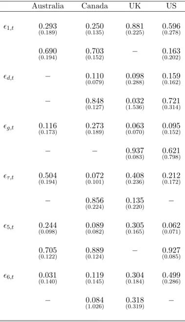
For each country, we estimate a 4-order VAR (m = 4). Table 1 reports the p-values associated with the McLeod-Li test statistic applied to the squared VAR residuals. In the vast majority of cases, the test rejects the null hypothesis of absence of autocorrelation in the squared VAR residuals at 1, 2 and 4 lags. This result hints to the presence of conditional heteroscedasticity in the statistical innovations, which is likely to translate into time-varying conditional variances of the structural innovations.
Table 2 presents the estimates of the GARCH(1,1) parameters. For each country, the estimates indicate that the conditional variances of (at least) five structural innovations are time-varying, and 7We found the results to be robust when we measure the price of bonds using the return on 10-year treasury
that the conditional variances of the structural innovations are linearly independent, thus satisfying the order (necessary) and rank (sufficient) conditions for the identification of system(7). The table also shows that government spending shocks exhibit a conditional volatility that is moderately persistent for Australia and Canada, but highly persistent for the UK and the US– where the persistence is measured by the sum of the ARCH and GARCH coefficients. On the other hand, the conditional volatility of tax shocks is highly persistent for all the countries except the US. A more telling representation of these conditional variances is provided by Figure 1. The figure shows important time variation in the conditional variances of both fiscal and non-fiscal shocks, which often display alternating episodes of high and low volatility. These results corroborate the findings of earlier studies that documented the presence of conditional volatility in the time series of output (Fountas and Karanasos 2007), the nominal interest rate (Garcia and Perron 1996; Den Haan and Spear 1998; Fernand`ez-Villaverde et al. 2010), the exchange rate (Hsieh 1988, 1989, Engel and Hamilton 1990, Engel and Kim 1999), and fiscal variables (Fernand`ez-Villaverde et al. 2011).
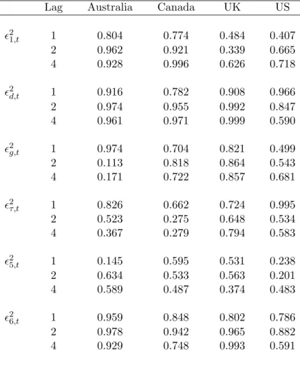
Does the GARCH(1,1) specification provide an adequate description of the process that governs the conditional variances of the structural innovations? To answer this question, we test whether there is any autocorrelation in the ratio of the squared structural innovations relative to their conditional variances. The Mcleod-Li test results, reported in Table 3, indicate that the null hypothesis of no autocorrelation cannot be rejected at any conventional level of significance for 1, 2 and 4 lags. This suggests that the GARCH(1,1) process is well specified.
Next, we turn to the estimates of the structural (bond-market) parameters, which we report in Table 4. The estimates of α indicate that the slope of the demand for newly issued government bonds is negative and statistically significant for all countries. The estimates of β are positive and statistically significant in all cases, indicating a positive relation between the demand for bonds and disposable income. The elasticity of demand for bonds with respect to the real exchange rate,
γ, is precisely estimated only for the US, but has the expected sign in all cases. The parameters
measuring the automatic/systematic responses of government spending and taxes to output, ηg and ητ respectively, are statistically significant for Canada and the US. The point estimates of ητ for
these two countries are substantially larger than the elasticity estimated by Blanchard and Perotti (2002) for the US, thus indicating that the systematic response of taxes to changes in output is quantitatively important. The parameters θg and θτ are mostly statistically significant, whereas
the opposite is true for ψg and ψτ. Finally, the scaling factor of government spending shocks, σg,
is smaller than that of tax shocks, στ.
The parametric restrictions implied by our model, i.e., a26 = 0, a36 = 0, a46 = 0, a24 =
−(a21+ a23), aa3222 = aa3525, and aa4222 = aa4525, are tested using a Wald test. The p-values associated with
the test statistic, reported in Table 5, indicate that these restrictions cannot be rejected at any conventional significance level for Australia, the UK, and the US. For Canada, these restrictions cannot be rejected only at the 4 percent (or lower) significance level. Since system (7) appears to be generally supported by the data, we henceforth refer to it as the unrestricted system and to its implications as the unrestricted ones.
3.2 Dynamic effects of tax shocks
Figure 2 depicts the dynamic effects of an unexpected tax cut on output, the primary budget deficit, the current account and the real exchange rate. The first observation that emerges from this figure is that there is, in general, a similarity in results between Australia and the UK on the one hand, and Canada and the US on the other hand. Notwithstanding that tax cut is much less persistent in Canada and the US than in Australia and the UK, it leads to a persistent and statistically significant increase in output in the former countries, whereas in the latter the output response is muted on impact and mostly statistically insignificant. The negative tax shock deteriorates the primary budget deficit in all four countries, but the effect is larger and much more persistent in Australia and the UK than in Canada and the US.
In contrast, the response of the current account in the former two countries is flat and indistin-guishable from zero. Hence, there is no evidence of twin deficits or twin divergence conditional on tax shocks for these two countries. On the other hand, the tax cut improves the current account in Canada, thus moving budget and external deficits in opposite directions–twin divergence. The opposite scenario occurs in the US, where the tax cut worsens both the budget deficit and the
current account-twin deficits. Therefore, there is no overwhelming evidence that, in a response to a tax shock, budget and external deficits move in tandem. In addition, these results provide little support to the hypothesis that the likelihood and magnitude of twin deficits increase with the degree of openness of an economy (see Corsetti and M¨uller 2006). Finally, Figure 2 shows that the real exchange rate is unresponsive, in a statistical sense, to the tax cut in Australia and the UK, but that it appreciates significantly in Canada and the US, although in the latter case, the exchange rate response ceases to be significant six quarters after the shock. These results constitute the first novelty of the present paper, as no empirical evidence exists about the effects of tax shocks on external variables in countries other than the US. Importantly, we find that the US is an outlier inasmuch as it is the only case where the effects of unexpected tax cuts are generally consistent with the predictions of standard economic models.
How do these results compare with those obtained by imposing the identifying restrictions used in earlier studies? Answering this question enables one to assess whether or not and to what extent those restrictions are innocuous. To conserve space, we restrict the comparison to the case of the US. Figure 3 superimposes on the unrestricted responses obtained for the US those implied by the recursive identification scheme discussed in Section 2 and by the two non recursive schemes employed by Kim and Roubini (KR) and Monacelli and Perotti (MP).8 In all cases, the system is estimated under the assumptions of conditional heteroscedasticity, so that any difference in results between the unrestricted and restricted systems would be solely attributed to the parametric restrictions on the coefficients of the matrix A. The figure shows that the three sets of identifying restrictions lead to important counterfactual implications. First, both the recursive and MP schemes severely understate the output response, predicting that it is essentially nil at all horizons, whereas the KR scheme implies that output actually falls in a response to a tax cut. Second, the three restricted systems imply that the unanticipated decrease in taxes worsens the budget primary deficit and improves the current account in the US, which contradicts the twin-deficit result obtained under the unrestricted specification. Finally, the tax cut leads to a real depreciation of the US dollar
8
under the three alternative identification schemes, whereas the unrestricted system predicts a real appreciation.9 These findings clearly show that imposing arbitrary parametric restrictions in order to achieve identification can lead to mistaken inference about a country’s external adjustment to tax shocks.
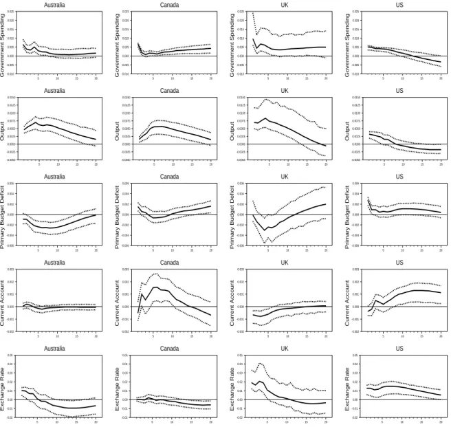
3.3 Dynamic effects of government spending shocks
The impulse responses to an expected increase in government spending shock are illustrated in Figure 4. The shock is expansionary in all four countries, leading to a persistent and statistically significant increase in output, except in the US, where the positive effect on output becomes statis-tically insignificant five quarters after the shock. The increase in government spending deteriorates the primary budget deficit in Canada and the US, and improves it in Australia and the UK,10 although in the latter case, the effect is mostly statistically insignificant. The current account remains unresponsive in Australia, improves in Canada and the US, and deteriorates in the UK. Thus, conditional on a government spending shock, there is stronger evidence of twin divergence than twin deficits. Again, we find little support for the hypothesis that twin deficits are more likely to occur in more open economies. Finally, Figure 4 indicates that the real exchange rate depreciates in a response to an unexpected increase in public spending, except in Canada, where the response is muted and statistically insignificant. This depreciation contradicts the predictions of standard open-economy models.
Figure 5 compares the results for the US with those obtained from the identification schemes used in existing studies, namely the recursive and sign-restriction approaches. Note that the dy-namic responses to a government spending shock implied by the KR and MP are identical to those implied by the recursive approach, since all of these systems assume that government spending is predetermined with respect to any other variable and impose the same number of exclusion restric-tions. In implementing the sign-restriction approach, we imposed the following restrictions on the 9The results obtained under the KR identification scheme are consistent with those reported in Kim and Roubini
(2008), which are based on a shorter sample period.
10
It is possible to obtain an improvement in the budget deficit following an expansionary public spending shock because our specification allows for an endogenous adjustment in taxes following such a shock, whereas earlier approaches restrict the initial response of taxes to be nil.
dynamic responses to a positive government spending shock: (i) government spending increases for 4 quarters, (ii) the primary budget deficit (as a fraction of output) worsens for four quarters, (iii) output increases for two quarters, and (iv) the real price of bonds falls on impact.11
At short horizons, the results obtained from the recursive and sign-restriction approaches re-garding the response of the budget deficit and the current account to a government spending shock are generally similar to those obtained from the unrestricted specification. All three approaches predict a worsening of the budget deficit and an improvement of the current account in the US in response to an expansionary spending shock. At longer horizons, however, the two alternative approaches under-estimate the response of the current account. More important discrepancies exist when it comes to the response of the real exchange rate. While the recursive approach yields a real depreciation, the latter is much smaller in magnitude than that predicted by the unrestricted system, especially at short horizons (up to two years). The sign-restriction approach, on the other hand, predicts that the median exchange rate response is very small in magnitude and changes sign during the first 10 quarters after the shock, but that there is so much uncertainty about such a response, that one cannot in fact reject the hypothesis that it is actually nil. Together, the results imply that the “real exchange rate puzzle” is worse than one may think based on traditional approaches.
4.
Robustness Analysis
We now study the robustness of the results to alternative detrending methods and to an alternative sample period. Recall that the benchmark results discussed so far were obtained from a system in which variables are expressed as deviations from a quadratic trend, and which is estimated over the post-1973 period. In this section, we report results based on systems in which variables are expressed (i) in levels, (ii ) as deviations from a linear trend, (iii) in first differences (except the current account and the real exchange rate, which are expressed in levels). We also estimate the system (with quadratically detrended data) for the post-1980 period, given that some studies
11
These restrictions are very similar to those imposed by Enders, M¨uller, and Scholl (2011), though not exactly the same. The reason is that our estimated system differs slightly from theirs. The dynamic responses we obtain using this approach are nonetheless remarkably similar to those reported by these authors.
suggest the presence of a structural break around the year 1980 (see Perotti 2005). We again restrict our attention to the US and report the results in Figure 6 for the case of a tax shock, and in Figure 7 for the case of a government spending shock. In the case where the data is expressed in first differences, the reported responses are those of the variables in levels and are obtained by cumulating the responses of the variables in first differences.
In general, the responses to a tax shock obtained under the alternative detrending methods are fairly similar to (and often statistically indistinguishable from) the benchmark responses, especially at short horizons. The only exceptions are the responses of output when the variables are expressed in levels and as deviations from a linear trend. On the other hand, the responses obtained for the post-1980 period are relatively smaller in magnitude than those pertaining to the entire sample period, although the wedge is generally not significantly large. An even stronger similarity in results between the benchmark and the alternative estimations is observed in the case of a government spending shock. The only notable difference concerns the response of the real exchange rate, which is smaller in magnitude in the post-1980 period than when the entire sample period is used in estimation.
To summarize, this robustness check confirms the message conveyed by the benchmark analysis regarding the adjustment of the US current account and exchange rate to fiscal-policy shocks: A surprise tax cut deteriorates the current account and appreciates the real exchange rate, whereas a surprise increase in public spending improves the current account with a delay and depreciates the real exchange rate.
5.
Conclusion
This paper has investigated the effects of fiscal policy shocks on the current account and the exchange rate using an empirical methodology that relaxes the commonly used identifying assump-tions, and which instead achieves identification by exploiting the conditional heteroscedasticity of the structural shocks within an SVAR.
four countries included in our sample, we found some similarities between Australia and the UK on the one hand, and Canada and the US on the other hand. More importantly, we found little support for the twin-deficit hypothesis regardless of the underlying fiscal shock. We also found that the effects of unexpected tax cuts are generally at odds with standard economic theory, except for the US. Finally, our results indicate that unexpected increases in public spending depreciates the currency in real terms in all but one country (Canada). While this puzzling depreciation (from the perspective of standard open-economy models) has also been documented by other studies, our results indicate that those studies severely understate the magnitude of the exchange rate response, thus suggesting that the “exchange rate puzzle” is worse than one might think based on traditional identification approaches.
Appendix: Data Construction and Sources
This appendix describes the data used in this paper. The sample covers the 1973-1 to 2008-4 period for Australia, Canada, the UK, and the US. For Australia and the UK, the data are taken from the International Financial Statistics (IFS) released by the International Monetary Funds, the Main Economic Indicators (MEI) and Economic Outlook (EO) released by the Organization for Economic Cooperation and Development, and from Datastream. Data for Canada are collected from the databases released by Statistics Canada (SC), while data for the US are taken from the National Income and Products Accounts (NIPA), the Federal Reserve Bank of Saint-Louis’ Fred database (FRED), and the Federal Reserve Statistical Releases (FRSR).
Output is measured by the nominal GDP (sources: EO for Australia and the UK, SC for Canada, and NIPA for the US) normalized by the GDP deflator (sources: EO for Australia and the UK, SC for Canada, and NIPA for the US). The price of bonds is constructed as the inverse of the gross real return, where the GDP deflator is used to deflate the gross nominal return. The nominal return is measured by the 90 day commercial bill rate for Australia (source: MEI), the 3-month treasury bill rate for Canada (source: SC), the UK (source: IFS), and the US (source: FRED). Except for the US, the exchange rate is defined as the consumer price index-based real effective exchange rate (source: MEI). For the US, the exchange rate is measured by the trade-weighted real exchange rate index against major currencies (source: FRSR). The current account (sources: EO for Australia and the UK, SC for Canada, and NIPA for the US) is expressed as a percentage of GDP. Government expenditures are measured by the sum of consumption and gross investment expenditures of the general government (sources: EO for Australia and the UK, SC for Canada, and NIPA for the US) normalized by the GDP deflator. Taxes are defined as total receipts of the general government less net transfers (sources: EO for Australia and the UK, SC for Canada, and NIPA for the US) normalized by GDP deflator. Output, government spending and taxes are expressed in per capita terms by dividing them by total population (sources: Datastream for Australia and the UK, SC for Canada and FRED for the US). Output, government spending, taxes, the price of bonds and the exchange rate are expressed in logarithm.
References
[1] Blanchard, Olivier J. and Roberto Perotti (2002), “An Empirical Characterization of the Dynamic Effect of Changes in Government Spending and Taxes on Output,” Quarterly Journal
of Economics 117: 1329–1368.
[2] Bouakez, Hafedh, Foued Chihi and Michel Normandin (2010), “Measuring the Effects of Fiscal Policy,” CIRP ´EE Working Paper No. 10–16.
[3] Corsetti, Giancarlo and Gernot J. M¨uller (2006), “Twin Deficits: Squaring Theory, Evidence and Common Sense,” Economic Policy 21: 597-638.
[4] Den Haan, Wouter J. and Scott A. Spear (1998), “Volatility Clustering in Real Interest Rates: Theory and Evidence,” Journal of Monetary Economics 41: 431-453.
[5] Enders, Zeno, Gernot J. M¨uller and Almuth Scholl (2011), “How Do Fiscal and Technology Shocks Affect Real Exchange Rates?: New evidence for the United States,” Journal of
Inter-national Economics 83: 53-69.
[6] Engel, Charles and James D. Hamilton (1990), “Long Swings in the Dollar: Are They in the Data and Do Markets Know It?,” American Economic Review 80: 713-869.
[7] Engel, Charles and Chang-Jin Kim (1999), “The Long-Run U.S./U.K. Real Exchange Rate,”
Journal of Money, Credit and Banking 31: 335-356.
[8] Fernandez-Villaverde, J´esus, Pablo Guerr´on-Quintana, Keith Kuester and Juan F. Rubio-Ram´ırez (2010), “Fiscal Volatility Shocks and Economic Activity,” manuscript.
[9] Fernandez-Villaverde, J´esus, Pablo Guerr´on-Quintana, Juan F. Rubio-Ram´ırez and Mart´ın Uribe (2011), “The Real Effects of Volatility Shocks,” American Economic Review,
[10] Fountas, Stilianos and Menelaos Karanasos (2007), “Inflation, Output Growth, and Nominal and Real Uncertainty: Empirical Evidence for the G7,” Journal of International Money and
Finance 26: 229-250.
[11] Garcia, Ren´e and Pierre Perron (1996), “An Analysis of the Real Interest Rate Under Regime Shifts,” The Review of Economics and Statistics 78: 111-125.
[12] Hsieh, David A. (1988), “The Statistical Properties of Daily Foreign Exchange Rates: 1974-1983,” Journal of International Economics 24: 129-145.
[13] Hsieh, David A. (1989), “Modeling Heteroscedasticity in Daily Foreign-Exchange Rates,”
Jour-nal of Business & Economic Statistics 7: 307-317.
[14] Kim, Soyoung and Nouriel Roubini (2008), “Twin Deficit or Twin Divergence? Fiscal Policy, Current Account, and Real Exchange Rate in the U.S”, Journal of International Economics 74: 362-383.
[15] Leeper, Eric M., Todd B. Walker and Shu-Chun Susan Yang (2008), “Fiscal Foresight: Ana-lytics and Econometrics,” manuscript, Indiana University.
[16] Mertens, Karel and Morten O. Ravn (2010), “Measuring the Impact of Fiscal Policy in the Face of Anticipation: A Structural VAR Approach,” The Economic Journal, 120: 393-413. [17] Monacelli, Tommaso and Roberto Perotti (2010), “Fiscal Policy, the Real Exchange Rate, and
Traded Goods,” The Economic Journal, 120: 437-461.
[18] M¨uller, Gernot J. (2008), “Understanding the Dynamic Effects of Government Spending on Foreign Trade,” Journal of International Money and Finance 27: 345-371.
[19] Perotti, Roberto (2005), “Estimating the Effects of Fiscal Policy in OECD Countries,”
Pro-ceedings, Federal Reserve Bank of San Francisco.
[21] Sims, Christopher and Tao Zha (1999), “Error Bands for Impulse Responses”, Econometrica, 67: 1113–1157.
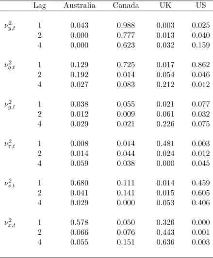
Table 1. Heteroscedasticity Test Results
Lag Australia Canada UK US
νy,t2 1 0.043 0.988 0.003 0.025 2 0.000 0.777 0.013 0.040 4 0.000 0.623 0.032 0.159 νq,t2 1 0.129 0.725 0.017 0.862 2 0.192 0.014 0.054 0.046 4 0.027 0.083 0.212 0.012 νg,t2 1 0.038 0.055 0.021 0.077 2 0.012 0.009 0.061 0.032 4 0.029 0.021 0.226 0.075 ντ,t2 1 0.008 0.014 0.481 0.003 2 0.014 0.044 0.024 0.012 4 0.059 0.038 0.000 0.045 νs,t2 1 0.680 0.111 0.014 0.459 2 0.041 0.141 0.015 0.605 4 0.029 0.000 0.053 0.406 νx,t2 1 0.578 0.050 0.326 0.000 2 0.066 0.076 0.443 0.001 4 0.055 0.151 0.636 0.003
Notes: Entries are the p-values associated with the McLeod-Li test statistic applied to the squared VAR residuals.
Table 2. Estimates of the GARCH(1,1) Parameters Australia Canada UK US ϵ1,t 0.293 (0.189) (0.135)0.250 (0.225)0.881 (0.278)0.596 0.690 (0.194) (0.152)0.703 − (0.202)0.163 ϵd,t − 0.110 (0.079) (0.288)0.098 (0.162)0.159 − 0.848 (0.127) (1.536)0.032 (0.314)0.721 ϵg,t 0.116 (0.173) (0.189)0.273 (0.070)0.063 (0.152)0.095 − − 0.937 (0.083) (0.798)0.621 ϵτ,t 0.504 (0.194) (0.101)0.072 (0.236)0.408 (0.172)0.212 − 0.856 (0.224) (0.220)0.135 − ϵ5,t 0.244 (0.098) (0.082)0.089 (0.165)0.305 (0.071)0.062 0.705 (0.122) (0.124)0.889 − (0.085)0.927 ϵ6,t 0.031 (0.140) (0.145)0.119 (0.184)0.304 (0.286)0.499 − 0.084 (1.026) (0.319)0.318 −
Notes: Entries are the estimates (standard errors) of the parameters of the GARCH(1,1) processes. For each structural innovation, the first and second rows refer to the ARCH and GARCH coeffi-cients, respectively. A dash (−) indicates that zero-restrictions are imposed to ensure that ∆1 and
Table 3. Specification Test Results
Lag Australia Canada UK US
ϵ21,t 1 0.804 0.774 0.484 0.407 2 0.962 0.921 0.339 0.665 4 0.928 0.996 0.626 0.718 ϵ2d,t 1 0.916 0.782 0.908 0.966 2 0.974 0.955 0.992 0.847 4 0.961 0.971 0.999 0.590 ϵ2 g,t 1 0.974 0.704 0.821 0.499 2 0.113 0.818 0.864 0.543 4 0.171 0.722 0.857 0.681 ϵ2τ,t 1 0.826 0.662 0.724 0.995 2 0.523 0.275 0.648 0.534 4 0.367 0.279 0.794 0.583 ϵ25,t 1 0.145 0.595 0.531 0.238 2 0.634 0.533 0.563 0.201 4 0.589 0.487 0.374 0.483 ϵ2 6,t 1 0.959 0.848 0.802 0.786 2 0.978 0.942 0.965 0.882 4 0.929 0.748 0.993 0.591
Notes: Entries are the p-values associated with the McLeod-Li test statistic applied to the squared structural innovations relative to their conditional variances.
Table 4. Estimates of the Structural Parameters
Parameter Australia Canada UK US
α 0.844 (0.186) (0.243)0.549 (0.195)1.066 (0.168)1.099 β 1.193 (0.120) (0.132)0.919 (0.294)0.986 (0.111)0.884 γ 0.073 (0.097) (0.104)0.012 (0.165)0.056 (0.104)0.267 ηg 0.484 (0.480) −0.237(0.741) 0.602 (1.230) (0.258)0.515 ητ 1.134 (1.197) 12.038(6.393) (1.914)1.152 (2.027)5.783 θg 0.732 (0.159) (0.192)0.425 (0.153)1.001 (0.179)0.371 θτ 1.176 (0.192) (0.726)1.001 (0.320)0.490 −0.076(0.859) ψg −0.186 (0.114) −0.037(0.056) 0.017 (0.301) (0.124)0.153 ψτ 1.372 (1.818) −2.571(2.472) 0.428 (2.734) −8.774(6.874) σd 0.019 (0.003) (0.007)0.018 (0.005)0.027 (0.005)0.011 σg 0.004 (0.005) (0.002)0.007 (0.017)0.005 (0.002)0.003 στ 0.036 (0.007) (0.027)0.056 (0.009)0.040 (0.012)0.025
Table 5. Test of the Parametric Restrictions
Australia Canada UK US
P-value 0.619 0.040 0.948 0.612
Note: Entries are the p-values of the χ2-distributed Wald test statistic associated with the restric-tions a26= 0, a36= 0, a46= 0, a24=−(a21+ a23), aa2232 = aa3525, and aa4222 = aa4525.
Australia G shock 1975 1980 1985 1990 1995 2000 2005 0.88 0.96 1.04 1.12 1.20 1.28 1.36 1.44 Canada G shock 1974 1979 1984 1989 1994 1999 2004 0.5 1.0 1.5 2.0 2.5 3.0 UK G shock 1975 1980 1985 1990 1995 2000 2005 0.00 0.25 0.50 0.75 1.00 1.25 US G shock 1975 1980 1985 1990 1995 2000 2005 0.72 0.84 0.96 1.08 1.20 1.32 1.44 1.56 1.68 1.80 Australia Tax shock 1974 1979 1984 1989 1994 1999 2004 0.0 0.8 1.6 2.4 3.2 4.0 4.8 5.6 Canada Tax shock 1974 1979 1984 1989 1994 1999 2004 0.6 0.8 1.0 1.2 1.4 1.6 1.8 2.0 UK Tax shock 1974 1979 1984 1989 1994 1999 2004 0 1 2 3 4 5 6 US Tax shock 1975 1980 1985 1990 1995 2000 2005 0.75 1.00 1.25 1.50 1.75 2.00 2.25 Australia Demand shock 1975 1980 1985 1990 1995 2000 2005 0.00 0.25 0.50 0.75 1.00 1.25 1.50 1.75 2.00 Canada Demand shock 1974 1979 1984 1989 1994 1999 2004 0.4 0.6 0.8 1.0 1.2 1.4 1.6 1.8 2.0 UK Demand shock 1974 1979 1984 1989 1994 1999 2004 0.5 1.0 1.5 2.0 2.5 3.0 3.5 4.0 4.5 US Demand shock 1975 1980 1985 1990 1995 2000 2005 0.50 0.75 1.00 1.25 1.50 1.75 2.00 2.25 Australia Shock 1 1975 1980 1985 1990 1995 2000 2005 0.00 0.25 0.50 0.75 1.00 1.25 1.50 1.75 2.00 Canada Shock 1 1974 1979 1984 1989 1994 1999 2004 0.0 0.5 1.0 1.5 2.0 2.5 3.0 UK Shock 1 1975 1980 1985 1990 1995 2000 2005 0.00 0.25 0.50 0.75 1.00 1.25 1.50 1.75 2.00 2.25 US Shock 1 1974 1979 1984 1989 1994 1999 2004 0.0 0.5 1.0 1.5 2.0 2.5 3.0 3.5 Australia Shock 5 1975 1980 1985 1990 1995 2000 2005 0.25 0.50 0.75 1.00 1.25 1.50 1.75 2.00 Canada Shock 5 1974 1979 1984 1989 1994 1999 2004 0.4 0.8 1.2 1.6 2.0 2.4 2.8 3.2 UK Shock 5 1974 1979 1984 1989 1994 1999 2004 0.5 1.0 1.5 2.0 2.5 3.0 US Shock 5 1974 1979 1984 1989 1994 1999 2004 0.4 0.5 0.6 0.7 0.8 0.9 1.0 1.1 1.2 Australia Shock 6 1975 1980 1985 1990 1995 2000 2005 0.96 0.98 1.00 1.02 1.04 1.06 1.08 1.10 1.12 Canada Shock 6 1974 1979 1984 1989 1994 1999 2004 0.8 0.9 1.0 1.1 1.2 1.3 1.4 1.5 1.6 UK Shock 6 1975 1980 1985 1990 1995 2000 2005 0.50 0.75 1.00 1.25 1.50 1.75 2.00 2.25 2.50 2.75 US Shock 6 1974 1979 1984 1989 1994 1999 2004 0.5 1.0 1.5 2.0 2.5 3.0
Australia Taxes 5 10 15 20 -0.05 -0.04 -0.03 -0.02 -0.01 0.00 0.01 0.02 Australia Output 5 10 15 20 -0.0075 -0.0050 -0.0025 0.0000 0.0025 0.0050 0.0075 0.0100 Australia
Primary Budget Deficit
5 10 15 20 -0.004 -0.002 0.000 0.002 0.004 0.006 0.008 0.010 Australia Current Account 5 10 15 20 -0.003 -0.002 -0.001 0.000 0.001 0.002 0.003 0.004 0.005 Australia Exchange Rate 5 10 15 20 -0.020 -0.015 -0.010 -0.005 0.000 0.005 0.010 0.015 0.020 Canada Taxes 5 10 15 20 -0.05 -0.04 -0.03 -0.02 -0.01 0.00 0.01 0.02 Canada Output 5 10 15 20 -0.0075 -0.0050 -0.0025 0.0000 0.0025 0.0050 0.0075 0.0100 Canada
Primary Budget Deficit
5 10 15 20 -0.004 -0.002 0.000 0.002 0.004 0.006 0.008 0.010 Canada Current Account 5 10 15 20 -0.003 -0.002 -0.001 0.000 0.001 0.002 0.003 0.004 0.005 Canada Exchange Rate 5 10 15 20 -0.020 -0.015 -0.010 -0.005 0.000 0.005 0.010 0.015 0.020 UK Taxes 5 10 15 20 -0.05 -0.04 -0.03 -0.02 -0.01 0.00 0.01 0.02 UK Output 5 10 15 20 -0.0075 -0.0050 -0.0025 0.0000 0.0025 0.0050 0.0075 0.0100 UK
Primary Budget Deficit
5 10 15 20 -0.004 -0.002 0.000 0.002 0.004 0.006 0.008 0.010 UK Current Account 5 10 15 20 -0.003 -0.002 -0.001 0.000 0.001 0.002 0.003 0.004 0.005 UK Exchange Rate 5 10 15 20 -0.020 -0.015 -0.010 -0.005 0.000 0.005 0.010 0.015 0.020 US Taxes 5 10 15 20 -0.05 -0.04 -0.03 -0.02 -0.01 0.00 0.01 0.02 US Output 5 10 15 20 -0.0075 -0.0050 -0.0025 0.0000 0.0025 0.0050 0.0075 0.0100 US
Primary Budget Deficit
5 10 15 20 -0.004 -0.002 0.000 0.002 0.004 0.006 0.008 0.010 US Current Account 5 10 15 20 -0.003 -0.002 -0.001 0.000 0.001 0.002 0.003 0.004 0.005 US Exchange Rate 5 10 15 20 -0.020 -0.015 -0.010 -0.005 0.000 0.005 0.010 0.015 0.020
Figure 2: Unrestricted dynamic responses to a negative tax shock.
Notes: The solid lines correspond to the dynamic responses to a negative tax shock extracted from the unrestricted system for each country. The dotted lines are the 68 percent confidence intervals computed using the Sims-Zha (1999) Bayesian procedure.
Recursive Taxes 5 10 15 20 -0.04 -0.03 -0.02 -0.01 0.00 0.01 0.02 Recursive Output 5 10 15 20 -0.008 -0.006 -0.004 -0.002 0.000 0.002 0.004 Recursive
Primary Budget Deficit 5 10 15 20
-0.003 -0.002 -0.001 0.000 0.001 0.002 0.003 0.004 0.005 0.006 Recursive Current Account 5 10 15 20 -0.0015 -0.0010 -0.0005 0.0000 0.0005 0.0010 0.0015 Recursive Exchange Rate 5 10 15 20 -0.015 -0.010 -0.005 0.000 0.005 0.010 0.015 Non Recursive (KR) Taxes 5 10 15 20 -0.04 -0.03 -0.02 -0.01 0.00 0.01 0.02 Non Recursive (KR) Output 5 10 15 20 -0.008 -0.006 -0.004 -0.002 0.000 0.002 0.004 Non Recursive (KR)
Primary Budget Deficit 5 10 15 20
-0.003 -0.002 -0.001 0.000 0.001 0.002 0.003 0.004 0.005 0.006 Non Recursive (KR) Current Account 5 10 15 20 -0.0015 -0.0010 -0.0005 0.0000 0.0005 0.0010 0.0015 Non Recursive (KR) Exchange Rate 5 10 15 20 -0.015 -0.010 -0.005 0.000 0.005 0.010 0.015 Non Recursive (MP) Taxes 5 10 15 20 -0.04 -0.03 -0.02 -0.01 0.00 0.01 0.02 Non Recursive (MP) Output 5 10 15 20 -0.008 -0.006 -0.004 -0.002 0.000 0.002 0.004 Non Recursive (MP)
Primary Budget Deficit 5 10 15 20
-0.003 -0.002 -0.001 0.000 0.001 0.002 0.003 0.004 0.005 0.006 Non Recursive (MP) Current Account 5 10 15 20 -0.0015 -0.0010 -0.0005 0.0000 0.0005 0.0010 0.0015 Non Recursive (MP) Exchange Rate 5 10 15 20 -0.015 -0.010 -0.005 0.000 0.005 0.010 0.015
Figure 3: Dynamic responses to a negative tax shock: Alternative identification schemes
Notes: The solid (dashed) lines correspond to the dynamic responses to a negative tax shock extracted from the unrestricted (alternative) system for the US. The dotted lines are the 68 percent confidence intervals computed using the Sims-Zha (1999) Bayesian procedure.
Australia Government Spending 5 10 15 20 -0.010 -0.005 0.000 0.005 0.010 0.015 0.020 0.025 Australia Output 5 10 15 20 -0.0050 -0.0025 0.0000 0.0025 0.0050 0.0075 0.0100 0.0125 0.0150 Australia
Primary Budget Deficit
5 10 15 20 -0.006 -0.004 -0.002 0.000 0.002 0.004 0.006 Australia Current Account 5 10 15 20 -0.002 -0.001 0.000 0.001 0.002 0.003 Australia Exchange Rate 5 10 15 20 -0.02 -0.01 0.00 0.01 0.02 0.03 0.04 0.05 Canada Government Spending 5 10 15 20 -0.010 -0.005 0.000 0.005 0.010 0.015 0.020 0.025 Canada Output 5 10 15 20 -0.0050 -0.0025 0.0000 0.0025 0.0050 0.0075 0.0100 0.0125 0.0150 Canada
Primary Budget Deficit
5 10 15 20 -0.006 -0.004 -0.002 0.000 0.002 0.004 0.006 Canada Current Account 5 10 15 20 -0.002 -0.001 0.000 0.001 0.002 0.003 Canada Exchange Rate 5 10 15 20 -0.02 -0.01 0.00 0.01 0.02 0.03 0.04 0.05 UK Government Spending 5 10 15 20 -0.010 -0.005 0.000 0.005 0.010 0.015 0.020 0.025 UK Output 5 10 15 20 -0.0050 -0.0025 0.0000 0.0025 0.0050 0.0075 0.0100 0.0125 0.0150 UK
Primary Budget Deficit
5 10 15 20 -0.006 -0.004 -0.002 0.000 0.002 0.004 0.006 UK Current Account 5 10 15 20 -0.002 -0.001 0.000 0.001 0.002 0.003 UK Exchange Rate 5 10 15 20 -0.02 -0.01 0.00 0.01 0.02 0.03 0.04 0.05 US Government Spending 5 10 15 20 -0.010 -0.005 0.000 0.005 0.010 0.015 0.020 0.025 US Output 5 10 15 20 -0.0050 -0.0025 0.0000 0.0025 0.0050 0.0075 0.0100 0.0125 0.0150 US
Primary Budget Deficit
5 10 15 20 -0.006 -0.004 -0.002 0.000 0.002 0.004 0.006 US Current Account 5 10 15 20 -0.002 -0.001 0.000 0.001 0.002 0.003 US Exchange Rate 5 10 15 20 -0.02 -0.01 0.00 0.01 0.02 0.03 0.04 0.05
Figure 4: Unrestricted dynamic responses to a positive government spending shock.
Notes: The solid lines correspond to the dynamic responses to a positive government spending shock extracted from the unrestricted system for each country. The dotted lines are the 68 percent confidence intervals computed using the Sims-Zha (1999) Bayesian procedure.
Recursive Government Spending 5 10 15 20 -0.004 -0.002 0.000 0.002 0.004 0.006 0.008 0.010 Recursive Output 5 10 15 20 -0.003 -0.002 -0.001 0.000 0.001 0.002 0.003 0.004 Recursive
Primary Budget Deficit 5 10 15 20
-0.005 -0.004 -0.003 -0.002 -0.001 0.000 0.001 0.002 0.003 0.004 Recursive Current Account 5 10 15 20 -0.0015 -0.0010 -0.0005 0.0000 0.0005 0.0010 0.0015 Recursive Exchange Rate 5 10 15 20 -0.015 -0.010 -0.005 0.000 0.005 0.010 0.015 0.020 Sign Government Spending 5 10 15 20 -0.004 -0.002 0.000 0.002 0.004 0.006 0.008 0.010 Sign Output 5 10 15 20 -0.003 -0.002 -0.001 0.000 0.001 0.002 0.003 0.004 Sign
Primary Budget Deficit 5 10 15 20
-0.005 -0.004 -0.003 -0.002 -0.001 0.000 0.001 0.002 0.003 0.004 Sign Current Account 5 10 15 20 -0.0015 -0.0010 -0.0005 0.0000 0.0005 0.0010 0.0015 Sign Exchange Rate 5 10 15 20 -0.015 -0.010 -0.005 0.000 0.005 0.010 0.015 0.020
Figure 5: Dynamic responses to a government spending shock: Alternative identification schemes.
Notes: The solid (dashed) lines correspond to the dynamic responses to a positive government spending shock extracted from the unrestricted (alternative) system for the US. The dotted lines are the 68 percent confidence intervals computed using the Sims-Zha (1999) Bayesian procedure for the recursive case and the 68 percent intervals of the admissible dynamic responses for the sign-restriction case.
Level Taxes 5 10 15 20 -0.03 -0.02 -0.01 0.00 0.01 0.02 0.03 Level Output 5 10 15 20 -0.0025 0.0000 0.0025 0.0050 0.0075 0.0100 0.0125 Level
Primary Budget Deficit
5 10 15 20 -0.005 -0.004 -0.003 -0.002 -0.001 0.000 0.001 0.002 0.003 0.004 Level Current Account 5 10 15 20 -0.005 -0.004 -0.003 -0.002 -0.001 0.000 0.001 Level Exchange Rate 5 10 15 20 -0.030 -0.025 -0.020 -0.015 -0.010 -0.005 0.000 0.005 0.010 Linear Trend Taxes 5 10 15 20 -0.03 -0.02 -0.01 0.00 0.01 0.02 0.03 Linear Trend Output 5 10 15 20 -0.0025 0.0000 0.0025 0.0050 0.0075 0.0100 0.0125 Linear Trend
Primary Budget Deficit
5 10 15 20 -0.005 -0.004 -0.003 -0.002 -0.001 0.000 0.001 0.002 0.003 0.004 Linear Trend Current Account 5 10 15 20 -0.005 -0.004 -0.003 -0.002 -0.001 0.000 0.001 Linear Trend Exchange Rate 5 10 15 20 -0.030 -0.025 -0.020 -0.015 -0.010 -0.005 0.000 0.005 0.010 First Difference Taxes 5 10 15 20 -0.03 -0.02 -0.01 0.00 0.01 0.02 0.03 First Difference Output 5 10 15 20 -0.0025 0.0000 0.0025 0.0050 0.0075 0.0100 0.0125 First Difference
Primary Budget Deficit
5 10 15 20 -0.005 -0.004 -0.003 -0.002 -0.001 0.000 0.001 0.002 0.003 0.004 First Difference Current Account 5 10 15 20 -0.005 -0.004 -0.003 -0.002 -0.001 0.000 0.001 First Difference Exchange Rate 5 10 15 20 -0.030 -0.025 -0.020 -0.015 -0.010 -0.005 0.000 0.005 0.010 Post-80 Sample Taxes 5 10 15 20 -0.03 -0.02 -0.01 0.00 0.01 0.02 0.03 Post-80 Sample Output 5 10 15 20 -0.0025 0.0000 0.0025 0.0050 0.0075 0.0100 0.0125 Post-80 Sample
Primary Budget Deficit
5 10 15 20 -0.005 -0.004 -0.003 -0.002 -0.001 0.000 0.001 0.002 0.003 0.004 Post-80 Sample Current Account 5 10 15 20 -0.005 -0.004 -0.003 -0.002 -0.001 0.000 0.001 Post-80 Sample Exchange Rate 5 10 15 20 -0.030 -0.025 -0.020 -0.015 -0.010 -0.005 0.000 0.005 0.010
Figure 6: Dynamic responses to a negative tax shock: Robustness analysis.
Notes: The solid lines correspond to the dynamic responses extracted from the unrestricted system for the US. The dashed lines correspond to the responses computed using alternative detrending methods and an alternative sample period. The dotted lines are the 68 percent confidence intervals computed using the Sims-Zha (1999) Bayesian procedure.
Level Government Spending 5 10 15 20 -0.006 -0.004 -0.002 0.000 0.002 0.004 0.006 0.008 Level Output 5 10 15 20 -0.004 -0.002 0.000 0.002 0.004 0.006 0.008 Level
Primary Budget Deficit
5 10 15 20 -0.003 -0.002 -0.001 0.000 0.001 0.002 0.003 0.004 0.005 Level Current Account 5 10 15 20 -0.0015 -0.0010 -0.0005 0.0000 0.0005 0.0010 0.0015 0.0020 0.0025 0.0030 Level Exchange Rate 5 10 15 20 -0.010 -0.005 0.000 0.005 0.010 0.015 0.020 Linear Trend Government Spending 5 10 15 20 -0.006 -0.004 -0.002 0.000 0.002 0.004 0.006 0.008 Linear Trend Output 5 10 15 20 -0.004 -0.002 0.000 0.002 0.004 0.006 0.008 Linear Trend
Primary Budget Deficit
5 10 15 20 -0.003 -0.002 -0.001 0.000 0.001 0.002 0.003 0.004 0.005 Linear Trend Current Account 5 10 15 20 -0.0015 -0.0010 -0.0005 0.0000 0.0005 0.0010 0.0015 0.0020 0.0025 0.0030 Linear Trend Exchange Rate 5 10 15 20 -0.010 -0.005 0.000 0.005 0.010 0.015 0.020 First Difference Government Spending 5 10 15 20 -0.006 -0.004 -0.002 0.000 0.002 0.004 0.006 0.008 First Difference Output 5 10 15 20 -0.004 -0.002 0.000 0.002 0.004 0.006 0.008 First Difference
Primary Budget Deficit
5 10 15 20 -0.003 -0.002 -0.001 0.000 0.001 0.002 0.003 0.004 0.005 First Difference Current Account 5 10 15 20 -0.0015 -0.0010 -0.0005 0.0000 0.0005 0.0010 0.0015 0.0020 0.0025 0.0030 First Difference Exchange Rate 5 10 15 20 -0.010 -0.005 0.000 0.005 0.010 0.015 0.020 Post-80 Sample Government Spending 5 10 15 20 -0.006 -0.004 -0.002 0.000 0.002 0.004 0.006 0.008 Post-80 Sample Output 5 10 15 20 -0.004 -0.002 0.000 0.002 0.004 0.006 0.008 Post-80 Sample
Primary Budget Deficit
5 10 15 20 -0.003 -0.002 -0.001 0.000 0.001 0.002 0.003 0.004 0.005 Post-80 Sample Current Account 5 10 15 20 -0.0015 -0.0010 -0.0005 0.0000 0.0005 0.0010 0.0015 0.0020 0.0025 0.0030 Post-80 Sample Exchange Rate 5 10 15 20 -0.010 -0.005 0.000 0.005 0.010 0.015 0.020
Figure 7: Dynamic responses to a positive government spending shock: Robustness analysis.
Notes: The solid lines correspond to the dynamic responses extracted from the unrestricted system for the US. The dashed lines correspond to the responses computed using alternative detrending methods and an alternative sample period. The dotted lines are the 68 percent confidence intervals computed using the Sims-Zha (1999) Bayesian procedure.