Annabi: HEC Montréal
Breton: HEC Montréal and GERAD François: HEC Montréal and CIRPÉE
Correspondance to: Michèle Breton, HEC Montreal, 3000 Côte-Sainte-Catherine, Montreal (QC), Canada H3T 2A7 [email protected]
Cahier de recherche/Working Paper 11-13
Game Theoretic Analysis of Negotiations under Bankruptcy
Amira Annabi
Michèle Breton
Pascal François
Abstract:
We extend the contingent claims framework for the levered firm in explicitly modeling the
resolution of financial distress under formal bankruptcy as a non-cooperative game
between claimants under the supervision of the bankruptcy judge. The identity of the
class of claimants proposing the first reorganization plan is found to be a key
determinant of the likelihood of liquidation and of the renegotiated value of claims. Our
quantitative results confirm the economic intuition that a bankruptcy design must
trade-off the initial priority of claims with the viability of reorganized firms.
Keywords: Bankruptcy procedure, game theory, dynamic programming
1
Introduction
The legal bankruptcy procedure is a major channel for resolving corporate financial distress. In the U.S. for instance, bankruptcydata.com has recorded more than 31,000 bankruptcy procedures since 1990. The 20 largest bankruptcy filings since 1980 totalled more than $1.8 billion.
One important alternative resolution of financial distress is out-of-court renegotiations. Early contingent claims models have analyzed this type of bargaining procedure using game theory (see in particular Anderson and Sundaresan, 1996, Mella-Barral and Perraudin, 1997, Mella-Barral, 1999, or Fan and Sundaresan, 2000). In these works, renegotiations are mod-elled as cooperative Nash bargaining games in which claimholders redistribute renegotiations surplus to avoid costly liquidation. Similar assumptions are made in other contingent claims models focusing on the U.S. bankruptcy procedure (namely, Chapter 11 of the Bankruptcy Code). These works include François and Morellec (2004), Galai, Raviv and Wiener (2007), and Broadie, Chernov and Sundaresan (2007).
The game theoretic modelling of a legal bankruptcy procedure requires a different spec-ification, however. Indeed, Brown (1989) and Gertner and Scharfstein (1991) argue that firms in financial distress will cease private negotiations and file bankruptcy when hold-out problems are severe — a view empirically supported by Gilson, John and Lang (1990) and Datta and Iskandar-Datta (1995). Consequently, it seems more appropriate to appeal to non-cooperative game theory to address the issue of renegotiations under legal bankruptcy. Another major difference between legal procedures and private workout is the monitoring of the renegotiation process by a bankruptcy judge. The empirical study of Chang and Schoar (2008) emphasizes the influence of the judge on the bankruptcy outcome. In a related work, Annabi, Breton and François (2010) explicitly account for Chapter 11 features into a game theoretic analysis and show how their calibrated model accurately reproduces stylized facts about outcomes of the U.S. bankruptcy procedure.
In this paper, we rely on the common legal features highlighted by White (1996) in her analysis of the bankruptcy procedures in the U.S., Canada, France, Germany and the U.K.
and examine the impact of the identity of the player having the first lead in the negotiation process. Specifically, we adapt the game theoretic modelling of Annabi et al. (2010) to a case where different types of players (shareholders, creditors, or Court-appointed trustee) have the opportunity to propose a first reorganization plan, submitted to a voting procedure. We find that the identity of the first proposer has a significant impact on what the various claimholders can expect to recover from the bankruptcy procedure, as well as on the viability of the reorganized firm. Specifically, our model explicitly quantifies the fundamental trade-off — initially put forward by Aghion, Hart and Moore (1992) — in bankruptcy procedure objectives: Depending on which type of claimholders is given the first mover advantage, the procedure succeeds in either preserving the initial priority of claims, or in allowing a financially sound firm to emerge. But none of the bankruptcy designs under study enable the procedure to meet the two objectives simultaneously.
The rest of the paper is organized as follows. Section 2 outlines the structure of the model. The negotiation game is formally detailed in Section 3. The algorithm to implement the model numerically is described in Section 4. We analyze our results in Section 5 and conclude in Section 6.
2
The negotiation model under bankruptcy
Under bankruptcy protection, the claimholders of a firm seek to renegotiate their claims and, depending on the success of this renegotiation, the firm can either be reorganized or liquidated. Accordingly, our modelling of the bargaining process under bankruptcy will successively address the characteristics of the bankrupt firm, the different players involved in the negotiation, the costs associated to the procedure, and the possible outcomes.
2.1
The bankrupt firm
The bankrupt firm files under bankruptcy at time 0. The value of its assets, denoted by , follow a geometric Brownian motion under the risk neutral probability measure. In accordance with a standard provision in bankruptcy codes (see e.g. White, 1996), we assume
that all payments to claimholders are suspended during the procedure, and resume if and once the firm emerges from bankruptcy at date ∗. Consequently, the payout rate for is nil between time 0 and time ∗. In case of successful reorganization, the firm resumes the payments to her claimants and we denote by the payout rate. Thus, the dynamics for the firm’s assets can be written as
= ⎧ ⎨ ⎩ + if 0 ≤ ∗ ( − ) + if ∗≤ (1)
where denotes the risk-free rate, the volatility of the assets, and is a standard
Brownian motion. Furthermore, time represents the date of a future financial distress event, which is assumed to eventually occur after a first successful reorganization.
2.2
The players
In practice, bankrupt firms may have a relatively complex capital structure involving multi-ple classes of claimants. To keep the negotiation process tractable, we focus on a bankrupt firm with two classes of debt with different priorities receiving a continuous coupon.
The negotiation process involves all the claimants of the firm and the bankruptcy judge. The creditors and equityholders are strategic participants, whereas the bankruptcy judge is a non-strategic player. Player will identify the class of shareholders, while Players and will identify the senior and junior creditors, respectively. Negotiation proceeds in successive bargaining rounds, where a class of claimants proposes a reorganization plan subject to the vote of other classes1. All claimants make their decisions independently, by taking into
account their best individual interest.
Although claimants are encouraged to voluntarily reach an agreement about the re-organization plan, the bankruptcy judge may interfere in the outcome of the negotiation process. She has a right to intervene at any bargaining round and her actions can consist in: (i) imposing a reorganization plan (cramdown), or (ii) liquidating the firm. Let denote
1In bankruptcy Codes where the management team stays in place during bankruptcy (e.g. the U.S. or
the probability of judge intervention at any given negotiation round. The judge intervenes to liquidate the firm when claimants unanimously reject the proposed plan, so that she deems any future negotiation doomed to fail. In the event of a cramdown, the judge can decide to impose a bargaining solution (with probability ) or the last proposed plan (with probability 1 − ). In the absence of judge intervention, the negotiation process carries on to the next round if players do not reach an agreement.
We finally assume homogenous information among players. In particular, all claimants and the judge observe the firm’s asset value process , and all claimants share the same exact anticipation of judge behavior (i.e. they all know the value of parameters and ).
2.3
Bankruptcy costs and outcomes
The bankruptcy process entails costs of financial distress, and also liquidation costs in case of negotiation failure. Both types of costs are borne by the firm. Considering for simplicity that all bargaining rounds are of equal length , we assume that a fixed amount 0,
proportional to the size of the firm and the length of the bargaining rounds, is due (in priority) at the end of each bargaining round, thus reducing the total value of the shares of the claimants in the reorganized firm. This amount accounts for both direct bankruptcy costs (such as legal fees) and indirect bankruptcy costs (such as productivity loss). As far as liquidation costs are concerned, we assume that a fraction 1 − of the ex-bankruptcy costs asset value is recovered in the case of a liquidation.
At the end of the negotiation process, either the firm is reorganized and resumes its operation with a new capital structure, or its assets are liquidated.
3
The negotiation game
3.1
Time-line
Our model spans the life of the firm, over an infinite horizon, starting from = 0 when a default event triggers the bankruptcy negotiation process. If the process results in a
reorganization, at date ∗, the reorganized firm continues operating until a second default event occurs at date . The firm stops operating, with a null recovery value, if at any time during the negotiation the value of the assets vanishes due to the accumulation of financial distress costs.
We model the negotiation process as a succession of sequential non-cooperative three player games, where one of the players, the leader, proposes a reorganization plan to the two others, the followers. If both followers approve the plan, or if the judge intervenes with a cramdown, a new reorganized firm emerges and continues its operations until . If the judge intervenes and imposes liquidation, the firm is liquidated according to the Absolute Priority Rule and the process terminates. Otherwise, the negotiation process continues to the next round, where the leadership is taken by another player. The process continues until either the firm is reorganized or liquidated (possibly with a null recovery value). For simplicity and tractability reasons, we assume that any further financial distress after the eventual reorganization leads to the liquidation of the firm.
This setting is similar to the negotiation model under the U.S. Chapter 11 bankruptcy procedure proposed in Annabi et al. (2010). Our model differs from the former by two essential features: First, we do not a priori limit the number of negotiation rounds, so that the negotiation game is solved over an infinite horizon. Second, we do not assume, as it is the case under Chapter 11, that the equityholders have the privilege of presenting the first plan, and we vary the order in which the players assume the leadership in the successive negotiation rounds. This allows us to analyze the impact of this specific feature on the length of the process, the ultimate recovery by the players, the probability of emergence, and the viability of the emerged firm.
The players strategies and the resulting outcomes depend on the observed level of the assets value, net of the financial distress costs, which defines the state of the system and is denoted by . We briefly recall the value function computation according to the various possible outcomes of a negotiation round.
3.2
Liquidation value
If the firm is liquidated, the assets of the firm, net of the financial distress costs, are disposed of at a proportional liquidation costs . The liquidation value of the firm is then given by
() = max [(1 − ) 0] , (2)
while the senior, junior and equityholders liquidation payoffs, according to Absolute Priority Rule, depend on the contractual coupons, denoted 0
(senior) and 0 (junior) and are given
respectively by () = min ∙ () 0 ¸ (3) () = min " max ∙ () − 0 0 ¸ 0 # (4) and () = max ∙ () − 0 ; 0 ¸ (5)
We denote by () =³(·) (·) (·)´the vector of liquidation values at assets value
3.2.1 Emergence value
If the firm emerges from financial distress at asset value , then the reorganized firm contin-ues its operations by distributing new coupons and to the senior and junior creditors
respectively, until further default and liquidation at time . The value at of the reorga-nized firm depends on the reorgareorga-nized coupon ≡ + and is given by
( ) = + Ã 1 − µ ¶ 1− ! − µ ¶ 1− (6)
where is the liquidation barrier and where = +++ , =
−−2 2 and = p 2 + 2.
The first term in (6) is the value of the assets at the emergence time, the second term is the present value of tax benefits of the operating firm, and the third term is the present value of liquidation costs.
Following Leland (1994), we assume that the liquidation barrier is determined so as to maximize equity value, and is given by
= (1 − )
. (7)
Rearranging (6), the total value of the firm at when the reorganized coupon is is given by: ( ) = Ã + − µ 1 − + ¶ µ (1 − ) ¶ 1 1− ! (8)
Denote ≡ (1−) Since this future liquidation leaves all the residual value to the
creditors, it is straightforward to compute the value of equity ( ) = µ − + (1 − )³ ´ 1 1− ¶ (9) and the value of senior and junior debt
( ) = µ 1 −³ ´ 1− ¶ + min h (1 − ) i ³ ´ 1− (10) ( ) = µ 1 −³ ´ 1− ¶ + maxh(1 − ) − 0 i ³ ´ 1− (11) as a function of the negotiated coupon. We denote by ( ) =
³
(·) (·) (·) ´ the vector of reorganization values at asset value when the reorganized coupon is ( ).
3.2.2 Bargaining solution value
Finally, we assume that the judge can impose in some cases an equitable plan, akin to the solutions of cooperative negotiation processes. Thus, we assume that this reorganization plan gives to each player at least his liquidation payoff, and equally shares the residual value among the claimants. Denoting ∗ = ∗+ ∗ the resulting total reorganized coupon, each claimant’s payoff then satisfies
() = 1 3 ¡ ( ∗) − (1 − ) ¢ | {z } Residual value + () ∈ { } (12)
This can be assimilated to the solution of a Nash bargaining game, where all claimant’s bargaining powers are equal.
3.2.3 Continuation values
If the firm is neither reorganized, nor liquidated at a given negotiation round, the continua-tion values are simply the expected values of the players future payoffs, taking into account the dynamics of the firm’s asset value and the equilibrium strategies. These future payoffs depend on the observed value of the firm’s asset, but also on the role (leader or follower) of the players in the upcoming negotiations. Accordingly, we assume that the order in which the players alternate in proposing plans is known in advance,2 and given by () identifying the identity of the player who takes the lead immediately after player (notice that with three players, there are only two possible such orderings). Continuation values are thus given, for ∈ { } by
( ) = −E[∗ ( ())] (13)
where ∗( ) = ³∗(·) ∗(·) ∗(·)´ denotes the vector of equilibrium outcomes of a negotiation round when the firms’ assets value is and Player is the leader, that is
∗ ( ) = ⎧ ⎪ ⎪ ⎪ ⎨ ⎪ ⎪ ⎪ ⎩
() if the firm is liquidated
( ) if the firm is reorganized with
( ) otherwise.
(14)
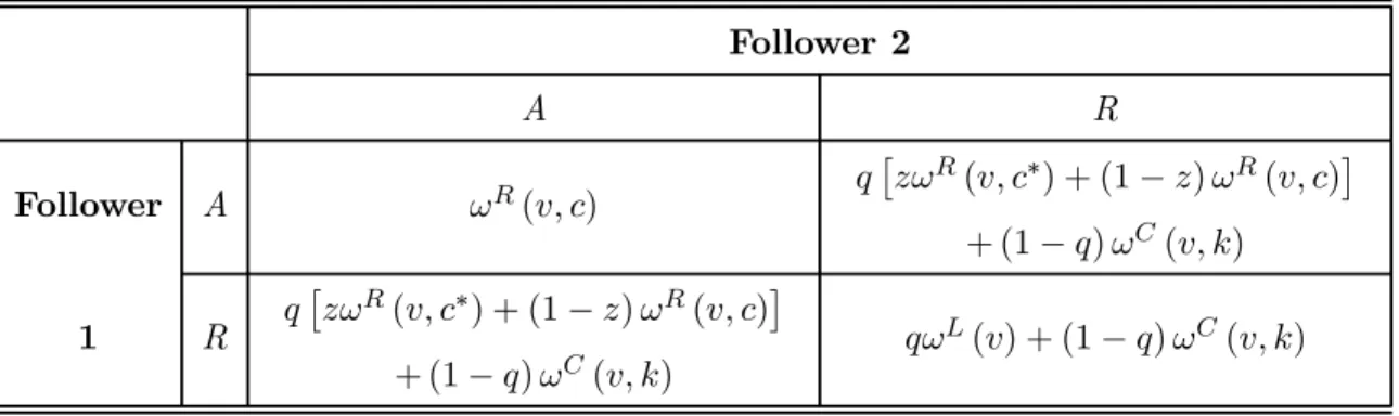
The Stackelberg/Nash equilibrium solution at a given negotiation round is obtained as in Annabi et al. (2010), where identifies the leader at this round. Thus, when the leader proposes his reorganization plan, he takes into account the equilibrium reactions of the two followers, where neither player has a unilateral incentive to change his strategy. Table 1 depicts the normal form representation of the game at a given round, between the claimant who proposes a reorganization plan and the other two claimants (Follower 1 and Follower 2), who vote on it.
2
One could also assume that the next leader will be chosen at random among the two followers. This alternate assumption gives similar qualitative results.
4
Numerical implementation
The function ∗( ) is the expected value, for claimant , of what he will ultimately recover from the bankruptcy process if the player who is currently the leader is Player and if the current value of assets is . This value function is defined recursively by the infinite horizon dynamic program (13)-(14) and is obtained by a value iteration algorithm. The value functions are evaluated on a grid of discretized asset values and interpolated by linear splines. Notice that the expectation of the resulting piecewise linear interpolation functions is then easy to obtain analytically, yielding the continuation values.
Upon convergence, the equilibrium strategies and payoffs of all players are obtained as a function of the asset value, net of bankruptcy costs, and of the identity of the leader. A Monte Carlo simulation of the negotiation period is then performed using these strategies to evaluate the expected length of the negotiation process, the probability of the various outcomes and the emergence values of the claimants according to the sequence of leaders starting from the first negotiation round. The algorithm is the following.
Algorithm 1. Initialization
Read parameter values, order of leadership, tolerance . Define a grid G on the asset’s value space.
Compute the liquidation value vector () ∈ G according to (3)-(5). Compute the bargaining solution vector () according to (12). Set ( ) = 0 for ∈ { } = 1 2 3 ∈ G.
2. Negotiation rounds
For ∈ { } compute the equilibrium outcome of the negotiation round where Player is the leader and where the payoff is given in Table 6.
(a) Find the coupon optimizing the payoff of the leader it both followers accept the proposed plan.
(b) Find the coupon optimizing the payoff of the leader if only one of the other followers accept the proposed plan.
(c) Compare the leader’s payoff for the four possible decision pairs of the follower. Record the equilibrium strategies ( ) and outcomes ∗( ), for ∈ { } according to (14).
3. Continuation values
(a) For ∈ { } interpolate ∗( ) and compute 0( ) according to (13).
(b) If¯¯0( ) ( )¯¯ for all and , go to step 4. (c) Otherwise, set ( ) = 0( ) and go to step 2.
4. Equilibrium outcomes
Simulate trajectories for the firm’s asset value using (1) for ∗ Using the
equilib-rium strategies (), record the final outcome on each trajectory.
5
Analysis of results
The literature on bankruptcy design highlights two important goals for the bankruptcy procedure (see e.g. White, 1989, or Aghion, Hart and Moore, 1992): (i) to preserve the bonding role of debt, and (ii) to filter out the economically sound firms that deserve to be reorganized (whereas the economically unsound firms should be liquidated). Accordingly, we can assess the quality of a bankruptcy procedure along three dimensions: (i) its ability to maintain the same priority among claimholders before and after reorganization (cf. the bonding role of debt), (ii) its ability to reorganize firms with high going concern value, and (iii) the costs incurred to pursue these two goals.
After calibrating the model in the next subsection, we compute the value functions of claims as well as the prevailing equilibrium as a function of asset value. Then, by simulating the dynamics of asset value, we can assess claimholders’ wealth (as the discounted
expected value of their claim at the end of the bankruptcy procedure). This allows us to examine how claimants share the value of the firm differently from their initial capital structure agreement. Simulations also enable us to compute the probabilities of the various bankruptcy outcomes and assess how much is the reorganized firm exposed to the risk of subsequent default.
5.1
Model calibration
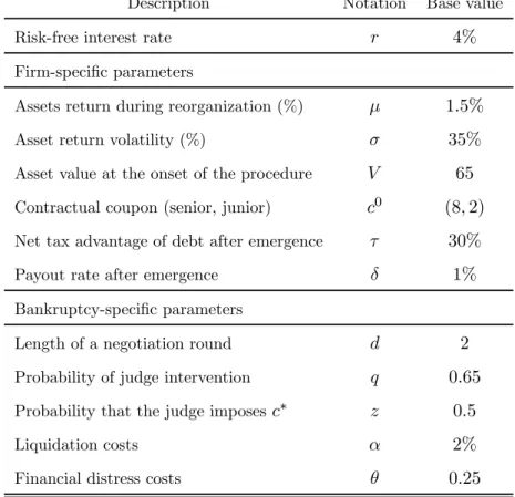
Definition, notation and base case values for various parameters are given in Table 2. We consider a firm whose assets grow at expected rate = 15% with a standard deviation of = 35%. These asset parameters are similar to those in Annabi et al. (2010). The firm is financed with a total coupon of 10. With a risk-free rate of = 4%, a corporate tax rate of = 30% and a payout rate of = 1%, the optimal default threshold, as defined in equation (7), is = 65098. Accordingly, we assume the firm files for bankruptcy when assets are worth 0 = 65.
As far as bankruptcy-specific parameters are concerned, we consider negotiation rounds with a two-year duration. The probability that the judge interferes if renegotiations fail is set at = 065. This relatively high value ensures that the threat of judge intervention is credible, but it does not reflect the actual probability of cramdown (which remains low, as it will be clear from our simulations). When the judge imposes a plan, chances are equal that it is the lately rejected plan or the “fair and equitable” plan, that is, = 05.
As far as the U.S. bankruptcy procedure is concerned, empirical studies report a rel-atively low estimate of median direct expenses of liquidation, ranging between 1.1% and 2.5% according to Ang, Chua and McConnell (1982), Lawless and Ferris (1997) and Bris, Zhu and Welch (2006). Non-U.S. evidence is more scarce and points towards slightly higher estimates. Ravid and Sundgren (1998) report median costs of 7.48% of assets for the Finnish liquidation procedure. Thorburn (2000) provides an estimate of 4.5% for the Swedish case. We choose to keep liquidation costs at a reasonably low level ( = 2%).
trustees and lawyers commissions, as well as indirect effects (much more difficult to estimate) mostly consisting of reputational costs and loss of investment opportunities. Given the lack of international evidence on financial distress costs, we will examine different values for parameter in our simulations with a base case value of 25% of initial asset value per year.
5.2
Value functions and equilibria
The bankruptcy procedure establishes a sequence in the proposals of plans. We therefore account for six different bankruptcy designs. For instance, the design labeled “E-S-J” gives equityholders the right to propose the first plan. Then senior (resp. junior) debtholders may propose a plan in the second (resp. third) round. If more than three rounds are needed, the sequence follows the same rotation among claimants.
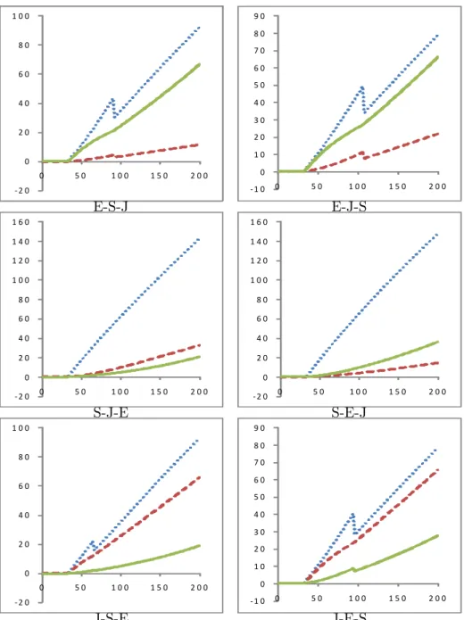
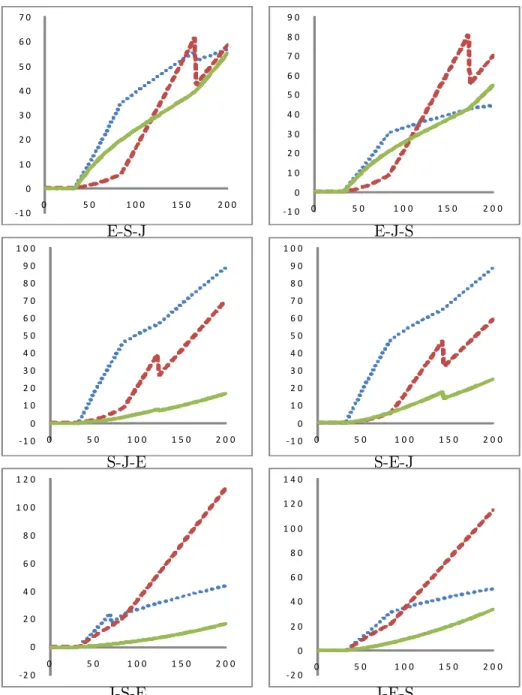
Figures 1 and 2 plot the value functions of equity, senior debt and junior debt as a function of asset value. In Figure 1, 80% of debt coupon is senior. In Figure 2, 80% of debt coupon is junior. The value functions are plotted for the six possible round sequences. They represent the expected value held by each claimholder at the end of the leader’s round. Their discontinuities result from a change in prevailing equilibrium. For instance in the top left graph in Figure 1 (representing the bankruptcy design E-S-J), equilibria are as follows: for asset value below 33, the firm is liquidated; for asset value between 33 and 35, the plan is rejected by one class of claimants; for asset value between 35 and 91, the plan is unanimously accepted; and for asset value above 91, the plan is rejected by one class of claimants.
When the leader is equityholders or junior creditors, they propose a plan that is unan-imously adopted for an intermediate range of asset values, which starts slightly above the liquidation region. In other words, the firm is reorganized under the leader’s plan for ∈ [ ] with and denotes the critical liquidation threshold. However, when
asset value is high (i.e. ), the leader proposes a plan that is unacceptable to one
class of claimants, who is better-off turning down the proposed plan in the hope of getting more in subsequent rounds (in particular when they become leader); when the asset value
is high, it is interesting for the leader to do so because there is a possibility that this plan be imposed by the judge, or that the process continues to a next round. If asset value is low and close to the liquidation region (i.e. ), senior creditors vote against the
plan as they know they will recover more from the liquidation procedure.
By contrast, when the leader is senior creditors, they propose a plan that is unanimously adopted for a range of asset values starting immediately above the liquidation region. In other words, the firm is reorganized under the leader’s plan for ∈ [ ]. Indeed, even
if asset value is low and close to the liquidation region, then both followers (equityholders and junior creditors) vote for the plan as they expect nothing from liquidation.
5.3
Firm and claim values
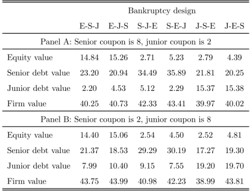
Table 3 reports the expected value of the three claims at the end of the bankruptcy pro-cedure, discounted at time zero. The sum of these three values represent the value of the firm as it enters bankruptcy.
We first observe that the bankruptcy design has an economically significant impact on firm value. Depending on the initial capital structure (panel A or B), firm value is impacted by around 10% because of the bankruptcy design. When debt is mostly senior (panel A), the most value enhancing bankruptcy designs are the ones allowing senior creditors to propose the first plan. By contrast, when debt is mostly junior (panel B), they are the ones where equityholders move first.
Table 3 also illustrates the impact of the bankruptcy procedure on the sharing rule of the value of the firm. It clearly indicates that the procedure gives a first mover advantage. In panel A for instance, senior creditors hold the biggest claim on firm value (they hold 80% of the total coupon). In the cases where they are given the right to propose the first plan (cases S-J-E and S-E-J), they benefit of the highest expected value for their claim. In all other cases, they have to make concessions to the two other classes of claimants, though they still keep the highest stake in the firm. In panel B (where senior creditors only hold 20% of the total coupon), junior debt value should be higher than that of senior debt.
Nevertheless, this is only the case where the bankruptcy procedure allows them to propose the first plan. In all other cases, they lose their rank as major stakeholders at the benefit of senior creditors and even equityholders in designs E-S-J and E-J-S.
Interestingly, when equityholders propose the first plan (as it is the case for Chapter 11 procedure for instance), they manage to end up being the second most important claimant, even though they rank last in priority.
Overall, we notice that out of the 12 possible bankruptcy designs, the initial priority rule of claims is maintained in 5 cases (S-J-E, J-S-E and J-E-S in panel A, and J-S-E and J-E-S in panel B), and is violated in the 7 other cases. Our simulations indicate that the initial priority rule of claims is best enforced when junior creditors are given the right to propose the first plan.
5.4
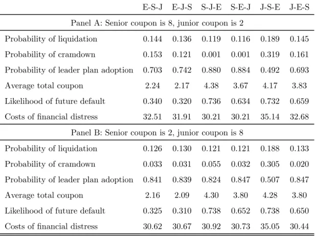
Bankruptcy outcomes
Table 4 summarizes the main bankruptcy outcomes generated by the model. For all 6 bankruptcy designs (characterized by the sequence of leadership in plan proposal), we report the probabilities for the three possible equilibria: liquidation, plan imposed by the judge (cramdown), or plan accepted by claimants’ vote. To gauge the financial health of the reorganized firm, we report its average total coupon as well as its “likelihood of future default”. This metric is essentially the ratio of the post-emergence default boundary over the post-emergence asset value.3 Formally, it is given by
(1 − )
where stands for the total coupon and is the simulated asset value at emergence. Table 4 finally reports the present value of average costs of financial distress, calculated as the costs per unit of time (i.e. costs per round scaled by round duration) multiplied by the average time spent under bankruptcy, and discounted at the risk-free rate.
3For each sample path of asset value, the likelihood of future default can be interpreted as the inverse of
Our model clearly indicates that the bankruptcy designs which allow equityholders to propose the first plan are the ones for which the firm emerges as the most viable going concern. In these cases indeed, both leverage (proxied by total coupon) and likelihood of future default are significantly lower.
By contrast, when senior debtholders move first, liquidation probabilities are smaller, firms remain highly levered, and the probability of them defaulting again in the near future is higher — all results that cast doubt on the ability of the bankruptcy procedure to efficiently filter-out poor performing firms. Bankruptcy designs where junior creditors move first share the same features, except that their liquidation rate is substantially higher.
We further note that our model cannot discriminate bankruptcy designs according to their implied costs of financial distress, as the time spent in bankruptcy is roughly the same across all possible designs.
Overall, our results show how conflicting the two bankruptcy procedure main goals are. If the legislator wants to put more emphasis on preserving the priority of claims, then by giving the initiative to junior creditors, the latter can better protect their weak rights. Conversely, if the legislator wants to put more emphasis on reorganizing sound firms, then by giving the initiative to equityholders, the latter can better de-leverage the firm and thus benefit of future upside performance.
5.5
Robustness checks
We generate the main bankruptcy outcomes with varying round duration (), probability of judge intervention () and costs of financial distress (). Results are reported in Table 5. The duration of negotiation rounds increases the probability of liquidation as more costs of financial distress accumulate (panel A). More costly rounds induce claimholders to be more “reasonable” in the plans they propose. As a result, for most bankruptcy designs, the firm emerges with less debt and in better financial health.
As expected, raising the probability of judge intervention increases the probability of cramdown (panel B). More counterintuitively, it also increases the time spent in
bank-ruptcy (and therefore the costs of financial distress), essentially because claimholders have a stronger incentive to “try their luck” on proposing an unreasonable plan that could be enforced by the judge. As a result, the firm emerges as a more levered and less viable going concern. This finding emphasizes the subtle role that the judge has to play in the procedure. A too credible threat of intervention, combined with the uncertainty about the cram-down plan, has the perverse effect of slowing down the convergence towards plan acceptance.
Finally, when costs of financial distress per period are higher (panel C), liquidation probability increases accordingly, and so does the probability of cramdown. As a matter of fact, claimholders have a stronger incentive to reach a quick agreement — rendering judge intervention less likely. Consequently, the total spent costs of financial distress actually decrease for most bankruptcy designs. Although the firm emerges with less debt, it is nevertheless more vulnerable to future default except when equityholders move first.
Even though the equilibrium probabilities may be significantly affected by changes in parameter values, our overall conclusion about bankruptcy designs remains robust. In all three panels in Table 5, the designs giving the initiative to senior creditors (resp. equity-holders) remain the ones in which firms emerge in greatest financial frailty (resp. health).
6
Conclusion
We have presented a contingent claims model of the levered firm in which the bankruptcy procedure is formally represented by a non-cooperative game between claimants under the supervision of the bankruptcy judge. One notable implication of our model is the explicit quantification of the two conflicting objectives (highlighted by the law and economics liter-ature) pursued by a bankruptcy procedure. These objectives are the maintenance of initial claims priority on one hand, and the ability to filter-out economically sound firms on the other hand. We show in this paper that the trade-off between these two objectives is greatly influenced by the identity of the class of claimants allowed to initiate the negotiations.
Our paper is also a first step towards modeling the impact of judge behavior on bank-ruptcy outcomes. Our analysis could be further developed by assigning the judge an explicit
objective function, thereby enriching the consequences of judge interference on the negoti-ation process. This is left for future research.
The procedure we are modeling captures essential legal features that are common to the bankruptcy laws prevailing in most OECD countries and others. Our approach is flexible enough to be calibrated to specific bankruptcy procedures throughout the world, leading to country-specific testable predictions. This is also left for future research.
References
[1] Aghion, P., Hart, O., and Moore, J., 1992. The Economics of Bankruptcy Reform. Journal of Law, Economics and Organization 8, 523—546.
[2] Anderson, R., and Sundaresan, S., 1996. The Design and Valuation of Debt Contracts. Review of Financial Studies 9, 37—68.
[3] Ang, J., Chua J., and McConnell, J., 1982. The Administrative Costs of Corporate Bankruptcy. Journal of Finance 37, 219—226.
[4] Annabi, A., Breton, M. and François, P., 2010. Resolution of Financial Distress under Chapter 11. Cahiers du GERAD G-2011-12 and CIRPÉE working paper#10-48. [5] Bris, A., Zhu, N., and Welch, I., 2006. The Costs of Bankruptcy. Journal of Finance
61, 1253—1303.
[6] Broadie, M., Chernov, M., and Sundaresan, S., 2007. Optimal Debt and Equity Values in the Presence of Chapter 7 and Chapter 11. Journal of Finance 62, 1341—1377. [7] Brown, D., 1989. Claimholder Incentive Conflicts in Reorganization: The Role of
Bank-ruptcy Law. Review of Financial Studies 2, 109—123.
[8] Chang, T., and Schoar, A., 2008. Judge Specific Differences in Chapter 11 and Firm Outcomes. Working Paper. MIT and NBER.
[9] Datta, S., and Iskandar-Datta, M. E., 1995. Reorganization and Financial Distress: An Empirical Investigation. Journal of Financial Research 18, 15—32.
[10] Fan, H., and Sundaresan, S., 2000. Debt Valuation, Renegotiation, and Optimal Divi-dend Policy. Review of Financial Studies 13, 1057—1099.
[11] François, P., and Morellec, E., 2004. Capital Structure and Asset Prices: Some Effects of Bankruptcy Procedures. Journal of Business 77, 387—411.
[12] Galai, D., Raviv, A., and Wiener, Z., 2007. Liquidation Triggers and the Valuation of Equity and Debt. Journal of Banking and Finance 31, 3604—3620.
[13] Gertner, R., and Scharfstein, D., 1991. A Theory of Workouts and the Effects of Re-organization Law. Journal of Finance 46, 1189—1222.
[14] Gilson, S., John, K., and Lang, L., 1990. Troubled Debt Restructurings: An Empirical Study of Private Reorganization of Firms in Default. Journal of Financial Economics 27, 315—353.
[15] Lawless, R. M. and Ferris, S. P., 1997. Professional Fees and Other Direct Costs in Chapter 7 Business Liquidations. Washington University Law Quarterly 75, 1207—1236. [16] Leland, H. E., 1994. Risky Debt, Bond Covenants and Optimal Capital Structure.
Journal of Finance 49, 1213—1252.
[17] Mella-Barral, P., 1999. The Dynamics of Default and Debt Reorganization. Review of Financial Studies 12, 535—578.
[18] Mella-Barral, P., and Perraudin, W., 1997. Strategic Debt Service. Journal of Finance 52, 531—556.
[19] Ravid, S. A., and Sundgren, S., 1998. The Comparative Efficiency of Small-Firm Bank-ruptcies: A Study of the US and the Finnish Bankruptcy Codes. Financial Management 27, 28—40.
[20] Thorburn, K. S., 2000. Bankruptcy Auctions: Costs, Debt Recovery, and Firm Survival. Journal of Financial Economics 58, 337—368.
[21] White, M., 1989. The Corporate Bankruptcy Decision. Journal of Economic Perspec-tives 3, 129—51.
[22] White, M., 1996. The Costs of Corporate Bankruptcy: A U.S.-European Comparison. In Bhandari J., Economic and Legal Perspectives, Cambridge UK: Cambridge Univer-sity Press.
Tables and figures
Follower 2 A R Follower A ( ) £ ( ∗) + (1 − ) ( )¤ + (1 − ) ( ) 1 R £ ( ∗) + (1 − ) ( )¤ + (1 − ) ( ) () + (1 − ) ( )Table 1: Normal form representation of the game at a given round.
This table shows the outcomes of a negotiation game at any given round, where the leader proposes a reorganization plan to the two other players. The followers decide independently whether to accept (A) or reject (R) the plan, which consists in a new reorganized coupon. If both followers accept the leader’s plan, then the firm is reorganized and the reorganized coupons are distributed. If both followers reject the plan, then the firm is liquidated by the bankruptcy judge with probability
, and the game moves to the next bargaining round otherwise. Finally, if the followers take opposite decisions on the leader’s plan, then the firm is reorganized by the judge with probability. In this case, the reorganized coupon can either be the bargaining solution ∗ with probability , or the Leader’s propositionwith probability(1 − ).
Description Notation Base value
Risk-free interest rate 4%
Firm-specific parameters
Assets return during reorganization (%) 15%
Asset return volatility (%) 35%
Asset value at the onset of the procedure 65
Contractual coupon (senior, junior) 0 (8 2)
Net tax advantage of debt after emergence 30%
Payout rate after emergence 1%
Bankruptcy-specific parameters
Length of a negotiation round 2
Probability of judge intervention 065
Probability that the judge imposes∗ 05
Liquidation costs 2%
Financial distress costs 025
Bankruptcy design
E-S-J E-J-S S-J-E S-E-J J-S-E J-E-S Panel A: Senior coupon is 8, junior coupon is 2
Equity value 14.84 15.26 2.71 5.23 2.79 4.39 Senior debt value 23.20 20.94 34.49 35.89 21.81 20.25 Junior debt value 2.20 4.53 5.12 2.29 15.37 15.38 Firm value 40.25 40.73 42.33 43.41 39.97 40.02
Panel B: Senior coupon is 2, junior coupon is 8
Equity value 14.40 15.06 2.54 4.50 2.52 4.81 Senior debt value 21.37 18.53 29.29 30.19 17.27 19.30 Junior debt value 7.99 10.40 9.15 7.55 19.20 19.70 Firm value 43.75 43.99 40.98 42.23 38.99 43.81
Table 3: Firm and claim values.
Table 3 reports the expected value of equity, senior debt and junior debt, discounted at initial date. Parameters are those in Table 2. Triplets of letters in column account for the bankruptcy design which consists in the sequence of leadership in reorganization plan proposal where E, S, and J stand for Equityholders, Senior debtholders and Junior debtholders, respectively. Reported results are based on 10,000 simulation paths.
Bankruptcy design
E-S-J E-J-S S-J-E S-E-J J-S-E J-E-S Panel A: Senior coupon is 8, junior coupon is 2
Probability of liquidation 0.144 0.136 0.119 0.116 0.189 0.145 Probability of cramdown 0.153 0.121 0.001 0.001 0.319 0.161 Probability of leader plan adoption 0.703 0.742 0.880 0.884 0.492 0.693 Average total coupon 2.24 2.17 4.38 3.67 4.17 3.83 Likelihood of future default 0.340 0.320 0.736 0.634 0.732 0.659 Costs of financial distress 32.51 31.91 30.21 30.21 35.14 32.68
Panel B: Senior coupon is 2, junior coupon is 8
Probability of liquidation 0.126 0.130 0.121 0.121 0.188 0.133 Probability of cramdown 0.033 0.031 0.055 0.032 0.305 0.020 Probability of leader plan adoption 0.841 0.839 0.824 0.847 0.507 0.847 Average total coupon 2.16 2.09 4.30 3.80 4.28 3.80 Likelihood of future default 0.325 0.310 0.738 0.652 0.738 0.650 Costs of financial distress 30.62 30.67 30.92 30.73 35.05 30.44
Table 4: Bankruptcy outcomes.
Table 4 reports the main bankruptcy outcomes of the model. Parameters are those in Table 2. Triplets of letters in column account for the bankruptcy design which consists in the sequence of leadership in reorganization plan proposal where E, S, and J stand for Equityholders, Senior debtholders and Junior debtholders, respectively. For all 6 bankruptcy designs, we report the prob-abilities for the three possible equilibria: liquidation, plan imposed by the judge (cramdown), or plan accepted by claimants’ vote. Also reported is the average total coupon as well as the “likelihood of future default”. This latter metric is computed as the ratio of the post-emergence default boundary over the post-emergence asset value. Table 4 finally reports the present value of average costs of financial distress, calculated as the costs per unit of time (i.e. costs per round scaled by round duration) multiplied by the average time spent under bankruptcy, and discounted at the risk-free rate. Reported results are based on 10,000 simulation paths.
Bankruptcy design
E-S-J E-J-S S-J-E S-E-J J-S-E J-E-S Panel A: Negotiation round duration ( = 1 = 3)
Prob. liquidation (0.011,0.459) (0.017,0.440) (0.000,0.422) (0.000,0.421) (0.027,0.558) (0.023,0.466) Prob. cramdown (0.471,0.162) (0.456,0.137) (0.000,0.037) (0.000,0.037) (0.594,0.400) (0.608,0.176) Prob. leader plan adoption (0.518,0.378) (0.526,0.423) (0.999,0.541) (0.999,0.543) (0.379,0.041) (0.368,0.357) Average total coupon (3.22,2.51) (3.10,2.46) (5.41,4.32) (4.36,3.74) (4.97,5.07) (4.62,4.23) Likelihood of future default (0.450,0.371) (0.411,0.349) (0.722,0.697) (0.585,0.595) (0.727,0.743) (0.648,0.642) Costs of financial distress (18.38,47.99) (18.26,47.24) (14.39,45.23) (14.39,45.35) (19.56,53.01) (19.72,48.30)
Panel B: Probability of judge intervention ( = 06 = 07)
Prob. liquidation (0.133,0.159) (0.132,0.150) (0.121,0.117) (0.119,0.119) (0.159,0.279) (0.136,0.185) Prob. cramdown (0.086,0.271) (0.051,0.244) (0.001,0.002) (0.000,0.001) (0.168,0.627) (0.067,0.405) Prob. leader plan adoption (0.780,0.570) (0.816,0.605) (0.877,0.881) (0.881,0.880) (0.673,0.093) (0.797,0.409) Average total coupon (2.11,2.34) (1.95,2.30) (4.30,4.39) (3.57,3.65) (4.08,4.66) (3.76,4.07) Likelihood of future default (0.317,0.376) (0.288,0.354) (0.722,0.742) (0.626,0.643) (0.720,0.735) (0.642,0.689) Costs of financial distress (31.69,33.61) (31.20,33.11) (30.18,30.20) (30.18,30.21) (33.43,38.09) (31.34,34.99)
Panel C: Costs of financial distress ( = 02 = 03)
Prob. liquidation (0.076,0.217) (0.075,0.210) (0.055,0.201) (0.056,0.218) (0.135,0.264) (0.087,0.222) Prob. cramdown (0.232,0.095) (0.197,0.066) (0.001,0.020) (0.001,0.019) (0.422,0.231) (0.271,0.098) Prob. leader plan adoption (0.692,0.688) (0.727,0.724) (0.944,0.779) (0.943,0.763) (0.442,0.505) (0.641,0.679) Average total coupon (2.56,1.97) (2.45,1.84) (4.66,4.14) (3.91,3.51) (4.51,3.98) (4.19,3.61) Likelihood of future default (0.363,0.330) (0.342,0.322) (0.726,0.777) (0.621,0.824) (0.722,0.767) (0.654,0.836) Costs of financial distress (33.56,31.44) (33.15,30.96) (30.26,30.37) (30.25,30.36) (36.97,33.70) (34.19,31.46)
Table 5: Bankruptcy outcomes — Robustness analysis.
Table 5 reports the main bankruptcy outcomes of the model for some parameters variations. Parameters are those in Table 2. Senior coupon is 8, junior coupon is 2. Definition of reported outcomes is the same as in Table 4. Reported results are based on 10,000 simulation paths.
‐ 2 0 0 2 0 4 0 6 0 8 0 1 0 0 0 5 0 1 0 0 1 5 0 2 0 0 E-S-J ‐ 1 0 0 1 0 2 0 3 0 4 0 5 0 6 0 7 0 8 0 9 0 0 5 0 1 0 0 1 5 0 2 0 0 E-J-S ‐ 2 0 0 2 0 4 0 6 0 8 0 1 0 0 1 2 0 1 4 0 1 6 0 0 5 0 1 0 0 1 5 0 2 0 0 S-J-E ‐ 2 0 0 2 0 4 0 6 0 8 0 1 0 0 1 2 0 1 4 0 1 6 0 0 5 0 1 0 0 1 5 0 2 0 0 S-E-J ‐ 2 0 0 2 0 4 0 6 0 8 0 1 0 0 0 5 0 1 0 0 1 5 0 2 0 0 J-S-E ‐ 1 0 0 1 0 2 0 3 0 4 0 5 0 6 0 7 0 8 0 9 0 0 5 0 1 0 0 1 5 0 2 0 0 J-E-S
Figure 1: Value functions of claims — debt mostly senior.
Value functions of equity, senior debt and junior debt are plotted as a function of asset value with straight, short-dashed and long-dashed lines, respectively. Parameters are those in Table 2. Senior coupon is 8 and junior coupon is 2. The caption of each figure indicates the sequence of leadership in reorganization plan proposal where E, S, and J stand for Equityholders, Senior debtholders and Junior debtholders, respectively.
‐1 0 0 1 0 2 0 3 0 4 0 5 0 6 0 7 0 0 5 0 1 0 0 1 5 0 2 0 0 E-S-J ‐ 1 0 0 1 0 2 0 3 0 4 0 5 0 6 0 7 0 8 0 9 0 0 5 0 1 0 0 1 5 0 2 0 0 E-J-S ‐ 1 0 0 1 0 2 0 3 0 4 0 5 0 6 0 7 0 8 0 9 0 1 0 0 0 5 0 1 0 0 1 5 0 2 0 0 S-J-E ‐ 1 0 0 1 0 2 0 3 0 4 0 5 0 6 0 7 0 8 0 9 0 1 0 0 0 5 0 1 0 0 1 5 0 2 0 0 S-E-J ‐ 2 0 0 2 0 4 0 6 0 8 0 1 0 0 1 2 0 0 5 0 1 0 0 1 5 0 2 0 0 J-S-E ‐ 2 0 0 2 0 4 0 6 0 8 0 1 0 0 1 2 0 1 4 0 0 5 0 1 0 0 1 5 0 2 0 0 J-E-S
Figure 2: Value functions of claims — debt mostly junior.
Value functions of equity, senior debt and junior debt are plotted as a function of asset value with straight, short-dashed and long-dashed lines, respectively. Parameters are those in Table 2. Senior coupon is 2 and junior coupon is 8. The caption of each figure indicates the sequence of leadership in reorganization plan proposal where E, S, and J stand for Equityholders, Senior debtholders and Junior debtholders, respectively.