HAL Id: hal-01757113
https://hal.archives-ouvertes.fr/hal-01757113v2
Preprint submitted on 26 Sep 2018
HAL is a multi-disciplinary open access
archive for the deposit and dissemination of
sci-entific research documents, whether they are
pub-lished or not. The documents may come from
teaching and research institutions in France or
abroad, or from public or private research centers.
L’archive ouverte pluridisciplinaire HAL, est
destinée au dépôt et à la diffusion de documents
scientifiques de niveau recherche, publiés ou non,
émanant des établissements d’enseignement et de
recherche français ou étrangers, des laboratoires
publics ou privés.
Time Blocks Decomposition of Multistage Stochastic
Optimization Problems
Pierre Carpentier, Jean-Philippe Chancelier, Michel de Lara, Tristan Rigaut
To cite this version:
Pierre Carpentier, Jean-Philippe Chancelier, Michel de Lara, Tristan Rigaut. Time Blocks
Decompo-sition of Multistage Stochastic Optimization Problems. 2018. �hal-01757113v2�
Noname manuscript No. (will be inserted by the editor)
Time Blocks Decomposition of Multistage Stochastic Optimization Problems
P. Carpentier ¨ J.-P. Chancelier ¨ M. De Lara ¨ T. Rigaut
the date of receipt and acceptance should be inserted later
Abstract Multistage stochastic optimization problems are, by essence, complex because their solutions are indexed both by stages (time) and by uncertainties (scenarios). Their large scale nature makes decomposition methods appealing. The most common approaches are time decomposition — and state-based resolution methods, like stochastic dynamic programming, in stochastic optimal control — and scenario decomposition — like progressive hedging in stochastic programming. We present a method to decompose multistage stochastic optimization problems by time blocks, which covers both stochastic programming and stochastic dynamic programming. Once established a dynamic programming equation with value functions defined on the history space (a history is a sequence of uncertainties and controls), we provide conditions to reduce the history using a compressed “state” variable. This reduction is done by time blocks, that is, at stages that are not necessarily all the original unit stages, and we prove a reduced dynamic programming equation. Then, we apply the reduction method by time blocks to two time-scales stochastic optimization problems and to a novel class of so-called decision-hazard-decision problems, arising in many practical situations, like in stock management. The time blocks decomposition scheme is as follows: we use dynamic programming at slow time scale where the slow time scale noises are supposed to be stagewise independent, and we produce slow time scale Bellman functions; then, we use stochastic programming at short time scale, within two consecutive slow time steps, with the final short time scale cost given by the slow time scale Bellman functions, and without assuming stagewise independence for the short time scale noises.
Keywords: multistage stochastic optimization, dynamic programming, decomposition, time blocks, two time-scales, decision-hazard-decision.
MSC: 90C06,90C39,93E20.
1 Introduction
Multistage stochastic optimization problems are, by essence, complex because their solutions are indexed both by stages (time) and by uncertainties. Their large scale nature makes decomposition methods appealing. The most common approaches are time decomposition — and state-based resolution methods, like stochastic dynamic programming, in stochastic optimal control — and scenario decomposition — like progressive hedging in stochastic programming.
On the one hand, stochastic programming deals with an underlying random process taking a finite number of values, called scenarios [10]. Solutions are indexed by a scenario tree, the size of which explodes with the number of stages, hence generally few in practice. However, to overcome this obstacle, stochastic programming takes advantage of scenario decomposition methods (progressive hedging [9]). On the other hand, stochastic control deals with a state model driven by a white noise, that is, the noise is made of
UMA, ENSTA ParisTech, Universit´e Paris-Saclay E-mail: [email protected] ¨ Universit´e Paris-Est, CERMICS (ENPC) E-mail: [email protected] ¨ Universit´e Paris-Est, CERMICS (ENPC) E-mail: [email protected] ¨ Efficacity E-mail: [email protected]
a sequence of independent random variables. Under such assumptions, stochastic dynamic programming is able to handle many stages, as it offers reduction of the search for a solution among state feedbacks (instead of functions of the past noise) [2, 8].
In a word, dynamic programming is good at handling multiple stages — but at the price of assuming that noises are stagewise independent — whereas stochastic programming does not require such assump-tion, but can only handle a few stages. Could we take advantage of both methods? Is there a way to apply stochastic dynamic programming at a slow time scale — a scale at which noise would be statis-tically independent — crossing over short time scale optimization problems where independence would not hold? This question is one of the motivations of this paper.
We will provide a method to decompose multistage stochastic optimization problems by time blocks. In Sect. 2, we present a mathematical framework that covers both stochastic programming and stochastic dynamic programming. First, in §2.1, we sketch the literature in stochastic dynamic programming, in order to locate our contribution. Second, in §2.2, we formulate multistage stochastic optimization prob-lems over a so-called history space, and we obtain a general dynamic programming equation. Then, we lay out the basic brick of time blocks decomposition, by revisiting the notion of “state” in Sect. 3. We lay out conditions under which we can reduce the history using a compressed “state” variable, but with a reduction done by time blocks, that is, at stages that are not necessarily all the original unit stages. We prove a reduced dynamic programming equation, and apply it to two classes of problems in Sect. 4. In §4.1, we detail the case of two time-scales stochastic optimization problems. In §4.2, we apply the reduction method by time blocks to a novel class consisting of decision-hazard-decision models. In the appendix, we relegate technical results, as well as the specific case of optimization with noise process.
2 Stochastic Dynamic Programming with Histories
We recall the standard approaches used to deal with a stochastic optimal control problem formulated in discrete time, and we highlight the differences with the framework used in this paper.
2.1 Background on Stochastic Dynamic Programming
We first recall the notion of stochastic kernel, used in the modeling of stochastic control problems. Let pX, Xq and pY, Yq be two measurable spaces. A stochastic kernel from pX, Xq to pY, Yq is a mapping ρ : X ˆ Y Ñ r0, 1s such that
– for any Y PY, ρp¨, Y q is X-measurable;
– for any x P X, ρpx, ¨q is a probability measure on Y.
By a slight abuse of notation, a stochastic kernel is also denoted as a mapping ρ : X Ñ ∆pYq from the measurable space pX, Xq towards the space ∆pYq of probability measures over pY, Yq, with the property that the function x P X ÞÑşY ρpx, dyq is measurable for any Y PY.
We now sketch the most classical frameworks for stochastic dynamic programming.
Witsenhausen Approach. The most general stochastic dynamic programming principle is sketched by Witsenhausen in [12]. However, we do not detail it as its formalism is too far from the following ones. We present here what Witsenhausen calls an optimal stochastic control problem in standard form (see [11]). The ingredients are the following:
1. time t “ t0, t0` 1, . . . , T ´ 1, T is discrete, with integers t0ă T ; 2. pXt0,Xt0q, . . . , pXT,XTq are measurable spaces (“state” spaces);
3. pUt0,Ut0q,. . . , pUT ´1,UT ´1q are measurable spaces (decision spaces);
4. Itis a subfield ofXt, for t “ t0, . . . , T ´ 1 (information);
5. ft: pXtˆ Ut,XtbUtq Ñ pXt`1,Xt`1q is measurable, for t “ t0, . . . , T ´ 1 (dynamics); 6. πt0 is a probability on pXt0,Xt0q;
7. j : pXT,XTq Ñ R is a measurable function (criterion).
With these ingredients, Witsenhausen formulates a stochastic optimization problem, whose solutions are to be searched among adapted feedbacks, namely λt : pXt,Xtq Ñ pUt,Utq with the property that
λ´1t pUtq Ă It for all t “ t0, . . . , T ´ 1. Then, he establishes a dynamic programming equation, where the Bellman functions are function of the (unconditional) distribution of the original state xtP Xt, and where the minimization is done over adapted feedbacks.
The main objective of Witsenhausen is to establish a dynamic programming equation for nonclassical information patterns.
Evstigneev Approach. The ingredients of the approach developed in [6] are the following: 1. time t “ t0, t0` 1, . . . , T ´ 1 is discrete, with integers t0ă T ;
2. pUt0,Ut0q,. . . , pUT ´1,UT ´1q are measurable spaces (decision spaces);
3. pΩ,Fq is a measurable space (Nature); 4. tFtut0,...,T ´1is a filtration ofF (information);
5. P is a probability on pΩ, Fq; 6. j : pśt“t0,...,T ´1Utˆ Ω,
Â
t“t0,...,T ´1UtbFq Ñ R is a measurable function (criterion).
With these ingredients, Evstigneev formulates a stochastic optimization problem, whose solutions are to be searched among adapted processes, namely random processes with values inś
t“t0,...,T ´1Ut and
adapted to the filtration tFtut0,...,T ´1. Then, he establishes a dynamic programming equation, where the
Bellman function at time t is an Ft-integrand depending on decisions up to time t (random variables) and where the minimization is done overFt-measurable random variables at time t.
The main objective of Evstigneev is to establish an existence theorem for an optimal adapted process (under proper technical assumptions, especially on the function j, that we do not detail here).
Bertsekas and Shreve Approach. The ingredients of the approach developed in [3] are the following: 1. time t “ t0, t0` 1, . . . , T ´ 1, T is discrete, with integers t0ă T ;
2. pXt0,Xt0q, . . . , pXT,XTq are measurable spaces (state spaces);
3. pUt0,Ut0q,. . . , pUT ´1,UT ´1q are measurable spaces (decision spaces);
4. pWt0,Wt0q,. . . , pWT,WTq are measurable spaces (Nature);
5. ft : pXtˆ Utˆ Wt,XtbUtbWtq Ñ pXt`1,Xt`1q is a measurable mapping, for t “ t0, . . . , T ´ 1 (dynamics);
6. ρt´1:t: Xt´1ˆ Ut´1Ñ ∆pWtq is a stochastic kernel, for t “ t0, . . . , T ´ 1;
7. Lt: Xtˆ Utˆ Wt`1Ñ R, for t “ t0, . . . , T ´ 1 and K : XT Ñ R, measurable functions (instantaneous and final costs).
With these ingredients, Bertsekas and Shreve formulate a stochastic optimization problem with time additive additive cost function over given state spaces, action spaces and uncertainty spaces (note that state and action spaces are assumed to be of fixed sizes when time varies, thus a “state” is a priori given). They introduce the notion of history at time t which consists in the states and the actions prior to t and study optimization problems whose solutions (policies) are to be searched among history feedbacks (or relaxed history feedbacks), namely sequences of mappings Xt0ˆ
śt´1
s“t0pUsˆ Xs`1q Ñ Ut. They identify
cases where no loss of optimality results from reducing the search to (relaxed) Markovian feedbacks Xt Ñ Ut. Then, they establish a dynamic programming equation, where the Bellman functions are function of the state xtP Xt, and where the minimization is done over controls utP Ut. For finite horizon problems, the mathematical challenge is to set up a mathematical framework (the Borel assumptions) for which optimal policies exists.
The main objective of Bertsekas and Shreve is to state conditions under which the dynamic program-ming equation is mathematically sound, namely with universally measurable Bellman functions and with universally measurable relaxed control strategies in the context of Borel spaces. The interested reader will find all the subtleties about Borel spaces and universally measurable concepts in [3, Chapter 7]. Puterman Approach. The ingredients of the approach developed in [8] are the following:
1. time t “ t0, t0` 1, . . . , T ´ 1, T is discrete, with integers t0ă T ; 2. pXt0,Xt0q, . . . , pXT,XTq are measurable spaces (state spaces);
3. pUt0,Ut0q,. . . , pUT ´1,UT ´1q are measurable spaces (decision spaces);
4. ρt´1:t: Xt´1ˆ Ut´1Ñ ∆pXtq is a stochastic kernel, for t “ t0, . . . , T ´ 1;
5. Lt: Xtˆ UtÑ R, for t “ t0, . . . , T ´ 1 and K : XT Ñ R, measurable functions (instantaneous and final costs).
Puterman shares most of his ingredients with Bertsekas and Shreve, but he does not require uncertainty sets and dynamics, as he directly considers state transition stochastic kernels. With these ingredients, Puterman formulates a stochastic optimization problem, whose solutions are to be searched among history feedbacks, namely sequences of mappings Xt0ˆ
śt´1
s“t0pUsˆ Xs`1q Ñ Ut. Then, he establishes
a dynamic programming equation, where the Bellman functions are function of the history ht P Xt0ˆ
śt´1
s“t0pUsˆ Xs`1q. He identifies cases where no loss of optimality results from reducing the search to
Markovian feedbacks XtÑ Ut. In such cases, the Bellman functions are function of the state xtP Xt, and the minimization in the dynamic programming equation is done over controls utP Ut.
The main objective of Puterman is to explore infinite horizon criteria, average reward criteria, the continuous time case, and to present many examples.
Approach in this Paper. The ingredients that we will use are the following: 1. time t “ t0, t0` 1, . . . , T ´ 1, T is discrete, with integers t0ă T ; 2. pUt0,Ut0q,. . . , pUT ´1,UT ´1q are measurable spaces (decision spaces);
3. pWt0,Wt0q,. . . , pWT,WTq are measurable spaces (Nature);
4. ρt´1:t: W0ˆ śt´1
s“0pUsˆ Ws`1q Ñ ∆pWtq is a stochastic kernel, for t “ t0, . . . , T ´ 1, 5. j : pW0ˆ
śT ´1
s“0pUsˆ Ws`1q,W0b ÂT ´1
s“0pUsbWs`1qq Ñ R is a measurable function (criterion). The main features of the framework developed in this paper are the following: the history at time t consists of all uncertainties and actions prior to time t (rather than states and actions); the cost is a unique function depending on the whole history, from initial time t0to the horizon T ; the probability distribution of uncertainty at time t depends on the history up to time t ´ 1. We will state a dynamic programming equation, where the Bellman functions are function of the history ht P W0ˆ
śt
s“0pUsˆ Ws`1q and where the minimization is done over controls utP Ut.
Our main objective is to establish a dynamic programming equation with a state, not at any time t P t0, . . . , T u, but at some specified instants 0 “ t0 ă t1ă ¨ ¨ ¨ ă tN “ T . The state spaces are not given a priori, but introduced a posteriori as image sets of history reduction mappings. With this, we can mix dynamic programming and stochastic programming.
Our framework is rather distant with the one of Evstigneev in [6]. It falls in the general framework developed by Witsenhausen (see [11] and [4, § 4.5.4]), except for the stochastic kernels (we are more general) and for the information structure (we are less general). Finally, our framework is closest to the one found in Bertsekas and Shreve [3] and Puterman [8], except for the state spaces, not given a priori, and for the criterion, function of the whole history.
2.2 Stochastic Dynamic Programming with History Feedbacks
We now present a framework that is adapted to both stochastic programming and stochastic dynamic programming. Time is discrete and runs among the integers t “ 0, 1, 2 . . . , T ´ 1, T , where T P N˚. For 0 ď r ď s ď T , we introduce the interval pr : sq “ tt P N | r ď t ď s u.
2.2.1 Histories and Feedbacks
We first define the basic and the composite spaces that we need to formulate multistage stochastic optimization problems. Then, we introduce a class of solutions called history feedbacks.
Histories and History Spaces. For each time t “ 0, 1, 2 . . . , T ´ 1, the decision ut takes its values in a measurable set Ut equipped with a σ-field Ut. For each time t “ 0, 1, 2 . . . , T , the uncertainty wt takes its values in a measurable set Wtequipped with a σ-fieldWt.
For t “ 0, 1, 2 . . . , T , we define the history space Ht equipped with the history field Htby Ht“ W0ˆ t´1 ź s“0 pUsˆ Ws`1q and Ht“W0b t´1 â s“0 pUsbWs`1q , t “ 0, 1, 2 . . . , T , (1) with the particular case H0“ W0,H0“W0. A generic element htP Htis called a history:
For 1 ď r ď s ď t, we introduce the pr : sq-history subpart
hr:s“ pur´1, wr, . . . , us´1, wsq , so that we have ht“ phr´1, hr:tq.
History Feedbacks. When 0 ď r ď t ď T ´ 1, we define a pr : tq-history feedback as a sequence tγsus“r,...,t of measurable mappings
γs: pHs,Hsq Ñ pUs,Usq . We call Γr:t the set of pr : tq-history feedbacks.
The history feedbacks reflect the following information structure. At the end of the time interval rt ´ 1, tr, an uncertainty variable wt is produced. Then, at the beginning of the time interval rt, t ` 1r, a decision-maker takes a decision ut, as follows
w0ù u0ù w1ù u1ù . . . ù wT ´1ù uT ´1ù wT . (2) 2.2.2 Optimization with Stochastic Kernels
We introduce a family of optimization problems with stochastic kernels. Then, we show how such prob-lems can be solved by stochastic dynamic programming.
In what follows, we say that a function is numerical if it takes its values in r´8, `8s (also called extended or extended real-valued function).
Family of Optimization Problems with Stochastic Kernels. To build a family of optimization problems over the time span t0, . . . , T ´ 1u, we require two ingredients:
– a family tρs´1:su1ďsďT of stochastic kernels
ρs´1:s: pHs´1,Hs´1q Ñ ∆pWsq , s “ 1, . . . , T , (3) that represents the distribution of the next uncertainty ws parameterized by past history hs´1 (see the chronology in (2)),
– a numerical function, playing the role of a cost to be minimized,
j : pHT,HTq Ñ r0, `8s , (4)
assumed to be nonnegative1 and measurable with respect to the fieldHT. We define, for any tγsus“t,...,T´1P Γt:T´1, a new family of stochastic kernels
ργt:T : pHt,Htq Ñ ∆pHTq ,
that capture the transitions between histories when the dynamics hs`1 “ `hs, us, ws`1˘ is driven by us“ γsphsq for s “ t, . . . , T ´1 (see Definition 5 in §A.2 for the detailed construction of ργr:t; note that ρ
γ t:T generates a probability distribution on the space HT of histories over the whole horizon t0, . . . , T u).
We consider the family of optimization problems, indexed by t “ 0, . . . , T ´ 1 and parameterized by the history htP Ht: inf γt:T ´1PΓt:T ´1 ż HT jph1 Tqρ γ t:Tpht, dh1Tq , @htP Ht, (5) the integral in the right-hand side of the above equation corresponding to the cost induced by the feedback γt:T ´1 when starting at time t with a given history ht. For all t “ 0, . . . , T ´ 1, we define the minimum value of Problem (5) by
Vtphtq “ inf γt:T ´1PΓt:T ´1 ż HT jph1 Tqρ γ t:Tpht, dh1Tq , @htP Ht, (6a) and we also define
VTphTq “ jphTq , @hT P HT . (6b)
The numerical function Vt: HtÑ r0, `8s is called the value function at time t. 1 We could also consider any j : H
t Ñ R, measurable bounded function, or measurable and uniformly bounded below
function. However, for the sake of simplicity, we will deal in the sequel with measurable nonnegative numerical functions. When jphTq “ `8, this materializes joint constraints between uncertainties and controls.
Bellman Operators and Dynamic Programming. We show that the value functions in (6) are Bellman functions, in that they are solution of the Bellman or dynamic programming equation.
For t “ 0, . . . , T , let L0`pHt,Htq be the space of universally measurable nonnegative numerical func-tions over Ht (see [3] for further details). For t “ 0, . . . , T ´ 1, we define the Bellman operator by, for all ϕ P L0
`pHt`1,Ht`1q and for all htP Ht, `Bt`1:tϕ˘phtq “ inf utPUt ż Wt`1 ϕpht, ut, wt`1qρt:t`1pht, dwt`1q . (7) Since ϕ P L0
`pHt`1,Ht`1q, we have that Bt`1:tϕ is a well defined nonnegative numerical function. The proof of the following theorem is inspired by [3], and given in §A.3.1.
Theorem 1 Assume that all the spaces introduced in §2.2.1 are Borel spaces, the stochastic kernels in (3) are Borel-measurable, and that the criterion j in (4) is a nonnegative lower semianalytic function.
Then, the Bellman operators in (7) map L0
`pHt`1,Ht`1q into L 0
`pHt,Htq Bt`1:t: L0
`pHt`1,Ht`1q Ñ L0`pHt,Htq ,
and the value functions Vt defined in (6) are universally measurable and satisfy the Bellman equation, or (stochastic) dynamic programming equation,
VT “ j , (8a)
Vt“ Bt`1:tVt`1, for t “ T ´1, . . . , 1, 0 . (8b)
This theorem is mainly inspired by [3], with the feature that the state xtis in our case the history ht, with the dynamics:
ht`1“`ht, ut, wt`1˘ . (9)
This very general dynamic programming result will be the basis of all future developments in this paper. In the sequel, we assume that all the assumptions of Theorem 1 are fulfilled, that is,
– all the spaces (like the ones introduced in §2.2.1) will be supposed to be Borel spaces,
– all the stochastic kernels (like the ones introduced in (3)) will be supposed to be Borel-measurable, – all the criteria (like the one introduced in (4)) will be supposed to be nonnegative lower semianalytic
functions.
3 State Reduction by Time Blocks and Dynamic Programming
In this section, we consider the question of reducing the history using a compressed “state” variable. Differing with traditional practice, such a variable may be not available at any time t P t0, . . . , T u, but at some specified instants 0 “ t0 ă t1 ă ¨ ¨ ¨ ă tN “ T . We have see in the previous section that the history ht is itself a canonical state variable in our framework with associated dynamics (9). However the size of this canonical state increases with t, which is a nasty feature for dynamic programming.
3.1 State Reduction on a Single Time Block
We first present the case where the reduction only occurs at two instants denoted by r and t: 0 ď r ă t ď T .
Definition 1 Let pXr,Xrq and pXt,Xtq be two measurable state spaces, θr and θt be two measurable reduction mappings
θr: HrÑ Xr, θt: HtÑ Xt, (10a) and fr:t be a measurable dynamics
The triplet pθr, θt, fr:tq is called a state reduction across pr : tq if we have θt ` phr, hr`1:tq ˘ “ fr:t`θrphrq, hr`1:t˘ , @htP Ht. (10c) The state reduction pθr, θt, fr:tq is said to be compatible with the family tρs´1:sur`1ďsďt of stochastic kernels (3) if
– there exists a reduced stochastic kernel r
ρr:r`1: XrÑ ∆pWr`1q , (11a) such that the stochastic kernel ρr:r`1 in (3) can be factored as
ρr:r`1phr, dwr`1q “ρrr:r`1`θrphrq, dwr`1˘ , @hrP Hr, (11b) – for all s “ r ` 2, . . . , t, there exists a reduced stochastic kernel
r
ρs´1:s: Xrˆ Hr`1:s´1Ñ ∆pWsq , (11c) such that the stochastic kernel ρs´1:s can be factored as
ρs´1:s ` phr, hr`1:s´1q, dws ˘ “ρrs´1:s ´ `θrphrq, hr`1:s´1˘, dws ¯ , @hs´1P Hs´1. (11d)
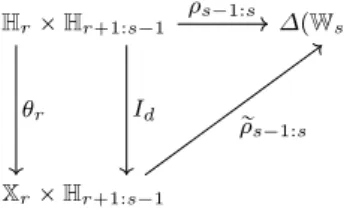
According to this definition, the triplet pθr, θt, fr:tq is a state reduction across pr : tq if and only if the diagram in Figure 1 is commutative; it is compatible if and only if the diagram in Figure 2 is commutative. Hrˆ Hr`1:t Ht Xrˆ Hr`1:t Xt θr Id Id θt fr:t
Fig. 1 Commutative diagram in case of state reduction pθr, θt, fr:tq
Hrˆ Hr`1:s´1 ∆pWsq Xrˆ Hr`1:s´1 θr Id ρs´1:s r ρs´1:s
Fig. 2 Commutative diagram in case of state reduction pθr, θt, fr:tq compatible with the family tρs´1:sur`1ďsďt
We define the Bellman operator across pt : rq Bt:r : L0`pHt,Htq Ñ L0`pHr,Hrq by
Bt:r “ Bt:t´1˝ ¨ ¨ ¨ ˝ Br`1:r, (12) where the one time step operators Bs:s´1, for r ` 1 ď s ď t are defined in (7).
The following proposition, whose proof is given in §A.3.2, is the key ingredient to formulate dynamic programming equations with a reduced state.
Proposition 1 Suppose that there exists a state reduction pθr, θt, fr:tq that is compatible with the fam-ily tρs´1:sur`1ďsďt of stochastic kernels (3) (see Definition 1). Then, there exists a reduced Bellman operator across pt : rq
r
Bt:r: L0`pXt,Xtq Ñ L0`pXr,Xrq , (13) such that, for allϕrtP L0`pXt,Xtq, we have that
` r Bt:rϕrt
˘
˝ θr“ Bt:rpϕrt˝ θtq . (14) For all measurable nonnegative numerical function ϕrt: XtÑ r0, `8s and for all xrP Xr, we have that
` r Bt:rϕrt ˘ pxrq “ inf urPUr ż Wr`1 r ρr:r`1pxr, dwr`1q inf ur`1PUr`1 ż Wr`2 r ρr`1:r`2pxr, ur, wr`1, dwr`2q . . . inf ut´1PUt´1 ż Wt r ϕt`fr:tpxr, ur, wr`1, . . . , ut´1, wtq ˘ r ρt´1:tpxr, ur, wr`1, . . . , ut´2, wt´1, dwtq . (15)
Proposition 1 can be interpreted as follows. Denoting by θ‹
t : L0`pXt,Xtq Ñ L0`pHt,Htq the operator defined by θ‹ tpϕrtq “ϕrt˝ θt, @ϕrtP L 0 `pXt,Xtq , the relation (14) rewrites
θ‹
r˝ rBt:r“ Bt:r˝ θ‹t ,
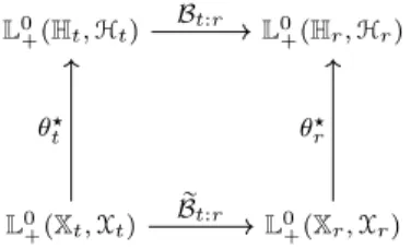
that is, Proposition 1 states that the diagram in Figure 3 is commutative.
L0`pHt,Htq L0`pHr,Hrq L0`pXt,Xtq L0`pXr,Xrq Bt:r θ‹ t r Bt:r θ‹ r
Fig. 3 Commutative diagram for Bellman operators in case of a compatible state reduction pθr, θt, fr:tq
3.2 State Reduction on Multiple Consecutive Time Blocks and Dynamic Programming Equations Proposition 1 can easily be extended to the case of multiple consecutive time blocks rti, ti`1s, i “ 0, . . . , N ´ 1, where
0 “ t0ă t1ă ¨ ¨ ¨ ă tN “ T . (16) Definition 2 Let tpXti,Xtiqui“0,...,N be a family of measurable state spaces, tθtiui“0,...,N be a family of measurable reduction mappings θti : Hti Ñ Xti, and fti:ti`1
(
i“0,...,N ´1 be a family of measurable dynamics fti:ti`1: Xtiˆ Hti`1:ti`1 Ñ Xti`1.
The triplet ptXtiui“0,...,N, tθtiui“0,...,N, fti:ti`1
(
i“0,...,N ´1q is called a state reduction across the con-secutive time blocks rti, ti`1s, i “ 0, . . . , N ´ 1 if every triplet pθti, θti`1, fti:ti`1q is a state reduction, for
i “ 0, . . . , N ´ 1.
The state reduction across the consecutive time blocks rti, ti`1s is said to be compatible with the family tρs´1:su1ďsďT of stochastic kernels given in (3) if every triplet pθti, θti`1, fti:ti`1q is compatible
Assuming the existence of a state reduction across the consecutive time blocks rti, ti`1s compatible with the family of stochastic kernels (3), we obtain the existence of a family of reduced Bellman operators across the consecutive pti`1: tiq as an immediate consequence of multiple applications of Proposition 1, that is, r Bti`1:ti : L 0 `pXti`1,Xti`1q Ñ L 0 `pXti,Xtiq , i “ 0, . . . , N ´ 1 ,
such that, for any functionϕrti`1 P L
0
`pXti`1,Xti`1q, we have that
` r
Bti`1:tiϕrti`1
˘
˝ θti“ Bti`1:tipϕrti`1˝ θti`1q .
We now consider the family of optimization problems (5) and the associated value functions (6). Thanks to the state reductions, we are able to state the following theorem which establishes dynamic programming equations across consecutive time blocks. Its proof is an immediate consequence of multiple applications of Theorem 1 and Proposition 1.
Theorem 2 Suppose that a state reduction ptXtiui“0,...,N, tθtiui“0,...,N, fti:ti`1
(
i“0,...,N ´1q exists across the consecutive time blocks rti, ti`1s, i “ 0, . . . , N ´ 1 as in (16), that is compatible with the fam-ily tρs´1:su1ďsďT of stochastic kernels given in (3).
Assume that there exists a reduced criterion r
j : XT Ñ r0, `8s , such that the cost function j in (4) can be factored as
j “ rj ˝ θtN .
We define the family of reduced value functions t rVtiui“0,...,N by
r
VtN “ rj , (18a)
r
Vti “ rBti`1:tiVrti`1, for i “ N ´ 1, . . . , 0 . (18b)
Then, the family tVtiui“0,...,N in (6) satisfies
Vti “ rVti˝ θti , i “ 0, . . . , N . (18c)
To obtain such a dynamic programming equation across time blocks, we needed the detour of Sect. 2, with a dynamic programming equation over the history space. Thus equipped, it is now possible to pro-pose a decomposition scheme for optimization problems with multiple time scales, using both stochastic programming and stochastic dynamic programming. We detail applications of this scheme in Sect. 4.
4 Applications of Time Blocks Dynamic Programming
We present in this section two applications of the state reduction result stated in Theorem 2.
The first one corresponds to a two time-scales optimization problem. A typical instance of such a problem is to optimize long-term investment decisions (slow time-scale) — for example the renewal of batteries in an energy system — but the optimal long-term decisions highly depend on short-term operating decisions (fast time-scale) — for example the way the battery is operated in real-time.
The second application corresponds to a class of stochastic multistage optimization problems arising often in practice, especially when managing stocks (dams for instance). The decision-maker takes two decisions at each time step t: at the beginning of the time interval rt, t ` 1r, the first decision (quantity of water to be turbinated to produce electricity for instance) is taken without knowing the uncertainty that will occur during the time step (decision-hazard framework); at the end of the time interval rt, t ` 1r, an uncertainty variable wt`1 is produced and the second decision (quantity of water to be released to avoid dam overflow for instance) is taken once the uncertainty at time step t is revealed (hazard-decision framework). This new class of problems is called decison-hazard-decision optimization problems.
4.1 Two Time-Scales Multistage Optimization Problems
In this class of problems, each time index t is represented by a couple pd, mq of indices, with d P t0, . . . , D ` 1u and m P t0, . . . , M u: we can think of the index d as an index of days (slow time-scale), and m as an index of minutes (fast time-scale). The corresponding set of time indices is thus
T “ t0, . . . , Du ˆ t0, . . . , M u Y tpD ` 1, 0qu . (19) At the end of every minute m´1 of every day d, that is, at the end of the time interval“pd, m´1q, pd, mq˘, 0 ď d ď D and 1 ď m ď M , an uncertainty variable wd,m becomes available. Then, at the beginning of the minute m, a decision-maker takes a decision ud,m. Moreover, at the beginning of every day d, an uncertainty variable wd,0 is produced, followed by a decision ud,0. The interplay between uncertainties and decision is thus as follows (compare the chronology with the one in (2)):
w0,0ù u0,0 ù w0,1ù u0,1ù ¨ ¨ ¨
¨ ¨ ¨ ù w0,M ´1ù u0,M ´1ù w0,Mù u0,M ù w1,0ù u1,0ù w1,1¨ ¨ ¨
¨ ¨ ¨ ù wD,M ù uD,M ù wD`1,0. We assume that a state reduction (as in Definition 2) is available at the beginning of each day d, so that it becomes possible to write dynamic programming equations by time blocks as stated by Theorem 2. Such state reductions will be for example available when the noises of the different days are stochastically independent.
We present the mathematical formalism to handle such type of problems. In this application, the difficulty to apply Theorem 2 is mainly notational.
Time Span. We consider the set T equipped with the lexicographical order
p0, 0q ă p0, 1q ă ¨ ¨ ¨ ă pd, M q ă pd ` 1, 0q ă ¨ ¨ ¨ ă pD, M ´ 1q ă pD, M q ă pD ` 1, 0q . (20a) The set T of couples in (19) is in one to one correspondence with the (linear) time span t0, . . . , T u, where
T “ pD ` 1q ˆ pM ` 1q ` 1 , (20b)
by the lexicographic mapping τ
τ : t0, . . . , T u Ñ T (20c)
t ÞÑ τ ptq “ pd, mq . (20d)
In the sequel, we will denote by pd, mq P T the element of t0, . . . , T u given by τ´1pd, mq “ dˆpM `1q`m: T Q pd, mq Ø τ´1pd, mq “ d ˆ pM ` 1q ` m P t0, . . . , T u . (20e) For pd, mq ď pd1, m1q, as ordered by the lexicographical order (20a), we introduce the time interval ppd, mq : pd1, m1qq “ tpd2, m2
q P T | pd, mq ď pd2, m2q ď pd1, m1q u.
History Spaces. For all pd, mq P t0, . . . , Duˆt0, . . . , M u, the decision ud,mtakes its values in a measurable set Ud,m equipped with a σ-field Ud,m. For all pd, mq P t0, . . . , Du ˆ t0, . . . , M u Y tpD ` 1, 0qu, the uncertainty wd,m takes its values in a measurable set Wd,m equipped with a σ-fieldWd,m.
With the identification (20e), for all pd, mq P T, we define the history space Hpd,mq
Hpd,mq“ W0,0ˆ U0,0ˆ W0,1ˆ ¨ ¨ ¨ ˆ Ud,m´1ˆ Wd,m, (21a) equipped with the history field Hpd,mq as in (1). For all d P t0, . . . , D ` 1u, we define the slow scale history hd element of the slow scale history space Hd
hd“ hpd,0qP Hd“ Hpd,0q, (21b) equipped with the slow scale history field Hd “Hpd,0q. For all d P t1, . . . , Du, we define the slow scale partial history space Hd:d`1
Hd:d`1“ Hpd,1q:pd`1,0q“ Ud,0ˆ Wd,1ˆ ¨ ¨ ¨ ˆ Ud,M ´1ˆ Wd,Mˆ Ud,Mˆ Wd`1,0, (21c) equipped with the associated slow scale partial history field Hd:d`1, the case d “ 0 being
Stochastic Kernels. Because of the jump from one day to the next, we introduce two families of stochastic kernels2:
– a family ρpd,M q:pd`1,0q(
0ďdďD of stochastic kernels across consecutive slow scale steps
ρpd,M q:pd`1,0q: Hpd,M qÑ ∆pWd`1,0q , d “ 0, . . . , D , (22a)
– a family ρpd,m´1q:pd,mq(
0ďdďD,1ďmďM of stochastic kernels within consecutive slow scale steps ρpd,m´1q:pd,mq: Hpd,m´1qÑ ∆pWd,mq , d “ 0, . . . , D , m “ 1, . . . , M . (22b)
History Feedbacks. A history feedback at index pd, mq P T is a measurable mapping γpd,mq: Hpd,mqÑ Upd,mq.
For pd, mq ď pd1, m1q, as ordered by the lexicographical order (20a), we denote by Γ
pd,mq:pd1,m1q the set of
ppd, mq : pd1, m1qq-history feedbacks.
Slow Scale Value Functions. We suppose given a nonnegative numerical function
j : HD`1Ñ r0, `8s , (23)
assumed to be measurable with respect to the fieldHD`1associated to HD`1.
For d “ 0, . . . , D, we build the new stochastic kernels ργpd,0q:pD`1,0q: HdÑ ∆pHD`1q (see Definition 5 in §A.2 for their construction), and we define the slow scale value functions
Vdphdq “ inf γPΓpd,0q:pD,M q ż HD`1 jph1D`1qρ γ pd,0q:pD`1,0qphd, dh 1 D`1q , @hdP Hd, (24a) VD`1“ j . (24b)
For d “ 0, . . . , D, we define a family of slow scale Bellman operators across pd ` 1 : dq Bd`1:d: L0`pHd`1,Hd`1q Ñ L
0
`pHd,Hdq , d “ 0, . . . , D , (25a) by
Bd`1:d“ Bpd`1,0q:pd,0q“ Bpd`1,0q:pd,M q˝ Bpd,M q:pd,M ´1q˝ . . . ˝ Bpd,1q:pd,0q. (25b) Then, applying repeatedly Theorem 1 leads to the fact that the family tVdud“0,...,D`1of slow scale value functions (24) satisfies
VD`1“ j , (26a)
Vd“ Bd`1:dVd`1 , for d “ D, D ´ 1, . . . , 0 . (26b)
2
These families are defined over the time span t0, . . . , T u ” T by the identification (20e) in such a way that the notation is consistent with the notation (3).
Compatible State Reductions. We now rewrite Definition 2 in the context of the two time-scales problem. Definition 3 (Compatible slow scale reduction) Let tpXd,Xdqud“0,...,D`1be a family of measurable state spaces, tθdud“0,...,D`1 be family of measurable reduction mappings such that
θd: HdÑ Xd,
and tfd:d`1ud“0,...,D be a family of measurable dynamics such that fd:d`1: Xdˆ Hd:d`1Ñ Xd`1.
The triplet `tXdud“0,...,D`1, tθdud“0,...,D`1, tfd:d`1ud“0,...,D˘ is said to be a slow scale state reduction if for all d “ 0, . . . , D θd`1 ` phd, hd:d`1q ˘ “ fd:d`1`θdphdq, hd:d`1˘ , @phd, hd:d`1q P Hd`1 .
The slow scale state reduction `tXdud“0,...,D`1, tθdud“0,...,D`1, tfd:d`1ud“0,...,D˘ is said to be compat-ible with the two families ρpd,M q:pd`1,0q(
0ďdďD and ρpd,m´1q:pd,mq (
0ďdďD,1ďmďM of stochastic kernels defined in (22a)–(22b) if for any d “ 0, . . . , D, we have that
– there exists a reduced stochastic kernel r
ρpd,M q:pd`1,0q: Xdˆ Hpd,0q:pd,M qÑ ∆pWd`1,0q , such that the stochastic kernel ρpd,M q:pd`1,0q in (22a) can be factored as
ρpd,M q:pd`1,0qphd,M, dwd`1,0q “ ρrpd,M q:pd`1,0q`θdphdq, hpd,0q:pd,M q, dwd`1,0 ˘
, @hd,M P Hpd,M q , – for each m “ 1, . . . , M , there exists a reduced stochastic kernel
r
ρpd,m´1q:pd,mq: Xdˆ Hpd,0q:pd,m´1qÑ ∆pWd,mq , such that the stochastic kernel ρpd,m´1q:pd,mq in (22b) can be factored as
ρpd,m´1q:pd,mqphd,m´1, dwd,mq “ρrpd,m´1q:pd,mq`θdphdq, hpd,0q:pd,m´1q, dwd,m˘ , @hd,m´1P Hpd,m´1q.
Dynamic Programming Equations. Using the reduced stochastic kernels of Definition 3, we apply Propo-sition 1 and obtain a family of slow scale reduced Bellman operators across pd ` 1 : dq
r
Bd`1:d: L0
`pXd`1,Xd`1q Ñ L0`pXd,Xdq , d “ 0, . . . , D . (29) We are now able to state the main result of this section.
Theorem 3 Assume that there exists a compatible slow scale state reduction `
tXdud“0,...,D`1, tθdud“0,...,D`1, tfd:d`1ud“0,...,D˘ and that there exists a reduced criterion rj : XD`1Ñ r0, `8s ,
such that the cost function j in (23) can be factored as j “ rj ˝ θD`1.
We define the family of reduced value functions t rVdud“0,...,D`1 by r
VD`1“ rj , (31a)
r
Vd“ rBd`1:dVrd`1 , for d “ D, . . . , 0 . (31b) Then, the family tVdud“0,...,D`1 of slow scale value functions (24) satisfies
Proof Since the triplet ptXdud“0,...,D`1, tθdud“0,...,D`1, tfd:d`1ud“0,...,Dq is a state reduction across the time blocks rpd, 0q, pd ` 1, 0qs, which is compatible with the family ρpd,0q:pd`1,0q
(
0ďdďD of stochastic kernels, the proof is an immediate consequence of Theorem 2.
Thanks to Theorem 3, we are able to replace the optimization problem formulated on the whole time set T by a sequence of D optimization subproblems formulated each on a single time block rpd, 0q, pd`1, 0qs. Moreover, the numerical burden of the method remains reasonable provided that the dimensions of the spaces Xdremain small, thus avoiding the curse of dimensionality. This is the benefit induced by dynamic programming which makes possible a time decomposition of the problem. However, to make the method operational, we need to compute the functions rVd, whose expression is available thanks to Proposition 1:
r Vdpxdq “ inf ud,0PUd,0 ż Wd,1 r ρpd,0q:pd,1qpxd, dwd,1q . . . inf ud,M ´1PUd,M ´1 ż Wd,M r ρpd,M ´1q:pd,M qpxd, ud,0, wd,1, ¨ ¨ ¨ , wd,M ´1, dwd,Mq inf ud,MPUd,M ż Wd`1,0 r Vd`1 ` r fd:d`1pxd, ud,0, wd,1, ¨ ¨ ¨ , ud,M ´1, wd,M, ud,M, wd`1,0q ˘ r ρpd,M q:pd`1,0qpxd, ud,0, wd,1, ¨ ¨ ¨ , wd,M, dwd`1,0q . (32) In many practical situations, this computation is tractable by using stochastic programming. For example, if the stochastic kernelsρrpd,mq:pd,m`1q do not depend on the past controls pud,0, ¨ ¨ ¨ , ud,m´1q, then it is possible to approximate the optimization problem (32) by using scenario tree techniques. Note that these last techniques do not require stagewise independence of the noises. We are thus able to take advantage of both the dynamic programming world and the stochastic programming world:
– use dynamic programming at slow time scale across consecutive slow time steps, when the slow time scale noises are supposed to be stochastically independent; produce slow time scale Bellman functions; – use stochastic programming at short time scale, within two consecutive slow time steps; the final short time scale cost is given by the slow time scale Bellman functions; no stagewise independence assumption is required for the short time scale noises.
4.2 Decision-Hazard-Decision Optimization Problems
We apply the reduction by time blocks to the so-called decision-hazard-decision dynamic programming. 4.2.1 Motivation for the Decision-Hazard-Decision Framework
We illustrate our motivation with a single dam management problem. We can model the dynamics of the water volume in a dam by
St`1“ mintS7, St´ qt` at`1u , (33) where t “ t0, t0` 1, . . . , T ´ 1 and
– S7 is the maximal dam volume,
– Stis the volume (stock) of water at the beginning of period rt, t ` 1r, – at`1 is the inflow water volume (rain, etc.) during rt, t ` 1r,
– qtis the turbined outflow volume during rt, t ` 1r (control variable), – decided at the beginning of period rt, t ` 1r,
– chosen such that 0 ď qtď St,
– supposed to depend on the stock Stbut not on the inflow water at`1.
The min operation in Equation (33) ensures that the dam volume always remains below its maximal capacity, but induces a non linearity in the dynamics.
Alternatively, we can model the dynamics of the water volume in a dam by
St`1“ St´ qt´ at`1´ rt`1, (34) where t “ t0, t0` 1, . . . , T ´ 1 and
– rt`1 is the spilled volume
– decided at the end of period rt, t ` 1r,
– supposed to depend on the stock Stand on the inflow water at`1, – and chosen such that 0 ď St´ qt` at`1´ rt`1ď S7.
Thus, with the formulation (34), we pay the price to add one control rt`1, but we obtain a linear model instead of the nonlinear model (33). This is especially interesting when using the stochastic dual dynamic programming (SDDP), for which the linearity of the dynamics is used to obtain the convexity properties required by the algorithm.
4.2.2 Decision-Hazard-Decision Framework
We consider stochastic optimization problems where, during the time interval between two time steps, the decision-maker takes two decisions. At the end of the time interval rs ´ 1, sr, an uncertainty vari-able w5
s is produced, and then, at the beginning of the time interval rs, s ` 1r, the decision-maker takes a head decision u7
s. What is new is that, at the end of the time interval rs, s ` 1r, when an uncertainty variable w5
s`1is produced, the decision-maker has the possibility to make a tail decision u5s`1. This lat-ter decision u5
s`1can be thought as a recourse variable for a two stage stochastic optimization problem that would take place inside the time interval rs, s ` 1r. We call w07 the uncertainty happening right before the first decision. The interplay between uncertainties and decisions is thus as follows (compare the chronology with the one in (2)):
w70 ù u70 ù w51 ù u51 ù u71 ù w25 ù . . . ù w5S´1 ù u5S´1 ù u7S´1 ù wS5 ù u5S . Let S P N˚. For each time s “ 0, 1, 2 . . . , S ´ 1, the head decision u7
s takes values in a measurable set U7
s, equipped with a σ-field U7s. For each time s “ 1, 2 . . . , S, the tail decision u5s takes values in measurable set U5
s, equipped with a σ-fieldU5s. For each time s “ 1, 2 . . . , S, the uncertainty ws5takes its values in a measurable set W5
s, equipped with a σ-fieldW5s. For time s “ 0, the uncertainty w 7
0 takes its values in a measurable set W70, equipped with a σ-fieldW
7 0.
Again, in this application, the difficulty to apply Theorem 2 is mainly notational. History Spaces. For s “ 0, 1, 2 . . . , S, we define the head history space
H7s“ W 7 0ˆ s´1 ź s1“0 ` U7s1ˆ W5s1`1ˆ U5s1`1˘ , (35a)
and its associated head history field H7
s. We also define, for s “ 1, 2 . . . , S, the tail history space H5s“ H
7 s´1ˆ U
7
s´1ˆ W5s, (35b)
and its associated tail history field H5 s.
Stochastic Kernels. We introduce a family of stochastic kernels tρs´1:su1ďsďS, with ρs´1:s: H7s´1Ñ ∆pW5
sq . (36)
History Feedbacks. For s “ 0, . . . , S ´ 1, a head history feedback at time s is a measurable mapping γ7
s: H7sÑ U7s. We call Γ7
s the set of head history feedbacks at time s, and we define Γ 7
s:S “ Γs7ˆ ¨ ¨ ¨ ˆ Γ 7
S. We also define, for all s “ 1, 2 . . . , S, a tail history feedback at time s as a measurable mapping
γ5
s: H5sÑ U5s. We call Γ5
Value Functions. We consider a nonnegative numerical function
j : H7S Ñ r0, `8s , (38)
assumed to be measurable with respect to the head history fieldH7S. For s “ 0, . . . , S , we define value functions by
Vsph7sq “ inf γ7PΓ7 s:S´1,γ5PΓ 7 s`1:S ż H7S jph1 Sqρ γ7,γ5 s:S ph7s, dh1Sq , @h7sP H7s, (39) where ργs:S7,γ5 has to be understood as ργs:S (see Definition 5), with
γsph7sq “ γs7ph7sq , @h7sP H7s, (40a) γs1ph5s1q “ ´ γs51ph5s1q, γ 7 s1`h5s1, γ5s1ph5s1q ˘¯ , @s1 “ s ` 1, . . . , S ´ 1 , @h5s1 P H5s1, (40b) γSph5Sq “ γS5ph5Sq , @h5S P H5S . (40c)
The following proposition, whose proof has been relegated in A.3.3, characterizes the dynamic pro-gramming equations in the decision-hazard-decision framework.
Proposition 2 For s “ 0, . . . , S ´ 1, we define the Bellman operator Bs`1:s: L0`pH 7 s`1,H 7 s`1q Ñ L 0 `pH7s,H7sq (41a)
such that, for all ϕ P L0`pH 7 s`1,H
7
s`1q and for all h7sP H7s, `Bs`1:sϕ˘ph7sq “ inf u7sPU7s ż W5s`1 ´ inf u5 s`1PU5s`1 ϕph7 s, u7s, ws`15 , u5s`1q ¯ ρs:s`1ph7s, dws`15 q . (41b)
Then the value functions (39) satisfy
VS “ j , (41c)
Vs“ Bs`1:sVs`1, @s “ 0, . . . , S ´ 1 . (41d) Compatible State Reductions. We now rewrite Definition 2 in the context of a decision-hazard-decision problem.
Definition 4 (Compatible state reduction) Let tXsus“0,...,Sbe a family of state spaces, tθsus“0,...,S be a family of measurable reduction mappings such that
θs: H7sÑ Xs,
and tfs:s`1us“0,...,S´1be a family of measurable dynamics such that fs:s`1: Xsˆ U7sˆ Ws`1ˆ U5s`1Ñ Xs`1.
The triplet`tXsus“0,...,S, tθsus“0,...,S, tfs:s`1us“0,...,S´1˘ is said to be a decision-hazard-decision state reduction if, for all s “ 0, . . . , S ´ 1, we have that
θs`1 ` phs, u7s, ws`1, u5s`1q ˘ “ fs:s`1`θsphsq, u7s, ws`1, u5s`1˘ , @phs, u7s, ws`1, u5s`1q P H7sˆ U7sˆ Ws`1ˆ U5s`1. The decision-hazard-decision state reduction is said to be compatible with the family tρs:s`1u0ďsďS´1 of stochastic kernels in (36) if there exists a family tρrs:s`1u0ďsďS´1 of reduced stochastic kernels
r
ρs:s`1: XsÑ ∆pWs`1q ,
such that, for each s “ 0, . . . , S ´ 1, the stochastic kernel ρs:s`1in (36) can be factored as ρs:s`1ph7s, dws`1q “ρrs:s`1`θsph
7
Dynamic Programming Equations. We state the main result of this section. Theorem 4 Assume that there exists a decision-hazard-decision state reduction `
tXsus“0,...,S, tθsus“0,...,S, tfs:s`1us“0,...,S´1˘ and that there exists a reduced criterion rj : XS Ñ r0, `8s ,
such that the cost function j in (38) can be factored as j “ rj ˝ θS.
We define a family of reduced Bellman operators across ps ` 1 : sq r
Bs`1:s: L0
`pXs`1,Xs`1q Ñ L0`pXs,Xsq , s “ 1, . . . , S ´ 1 , (45a) by, for any measurable function ϕ : Xr s`1Ñ r0, `8s,
p rBs`1:sϕqpxr sq “ inf u7sPU7s ż Ws`1 ´ inf u5 s`1PU5s`1 r ϕ`fs:s`1pxs, u7s, ws`1, u5s`1q ˘¯ r ρs:s`1pxs, dws`1q . (45b)
*We define the family of reduced value functions t rVsus“0,...,S by r
VS “ rj (46a)
r
Vs“ rBs`1:sVrs`1 for s “ S ´ 1, . . . , 0 . (46b) Then, the value functions Vsdefined by (39) satisfy
Vs“ rVs˝ θs, s “ 0, . . . , S . (47)
Proof It has been shown in the proof of Proposition 2 that the setting of a decision-hazard-decision problem was a particular kind of two time-scales problem. The proof of the theorem is then a direct application of Theorem 3.
Theorem 4 allows to develop dynamic programming equations in the decision-hazard-decision frame-work. Such equations can be solved using the stochastic dual dynamic programming (SDDP) algorithm provided that convexity of the value functions is preserved. This requires linearity in the dynamics, a feature that may be recovered by modeling the problem in the decision-hazard-decision framework as illustrated in §4.2.1.
5 Conclusion and Perspectives
As said in the introduction, decomposition methods are appealing to tackle multistage stochastic opti-mization problems, as they are naturally large scale. The most common approaches are time decompo-sition (and state-based resolution methods, like stochastic dynamic programming, in stochastic optimal control), and scenario decomposition (like progressive hedging in stochastic programming). One also finds space decomposition methods [1].
This paper is part of a general research program that consists in mixing different decomposition bricks. Here, we tackled the issue of mixing time decomposition (stochastic dynamic programming) with scenario decomposition. For this purpose, we have revisited the notion of state, and have provided a way to perform time decomposition but only accross specified time blocks. Inside a time block, one can then use stochastic programming methods, like scenario decomposition. Our time blocks decomposition scheme is especially adapted to multi time-scales stochastic optimization problems. In this vein, we have shown its application to two time-scales and to the novel class of decision-hazard-decision problems.
We are currently working on how to mix time decomposition (stochastic dynamic programming) with space/units decomposition.
Acknowledgements. We thank Roger Wets for the fruitful discussions about the possibility of mixing stochastic dynamic programming with progressive hedging. We thank an anonymous reviewer for challenging our first version of the paper: the current version has been deeply restructured.
A Technical Details and Proofs
In this section, we provide technical details, constructions and proofs of results in the paper.
A.1 Histories, Feedbacks and Flows
We introduce the notations
Wr:t“ t ź s“r Ws, 0 ď r ď t ď T (48a) Ur:t“ t ź s“r Us, 0 ď r ď t ď T ´ 1 (48b) Hr:t“ t´1 ź s“r´1 pUsˆ Ws`1q “ Ur´1ˆ Wrˆ ¨ ¨ ¨ ˆ Ut´1ˆ Wt, 1 ď r ď t ď T . (48c)
Let 0 ď r ď s ď t ď T . From a history htP Ht, we can extract the pr : sq-history uncertainty part
rhtsWr:s“ pwr, . . . , wsq “ wr:sP Wr:s, 0 ď r ď s ď t , (49a)
the pr : sq-history control part (notice that the indices are special)
rhtsU
r:s“ pur´1, . . . , us´1q “ ur´1:s´1P Ur´1:s´1, 1 ď r ď s ď t , (49b)
and the pr : sq-history subpart
rhtsr:s“ pur´1, wr, . . . , us´1, wsq “ hr:sP Hr:s, 1 ď r ď s ď t , (49c)
so that we obtain, for 0 ď r ` 1 ď s ď t,
ht“ pw0, u0, w1, . . . , ur´1, wr loooooooooooooooomoooooooooooooooon hr , ur, wr`1, . . . , ut´2, wt´1, ut´1, wt looooooooooooooooooooooomooooooooooooooooooooooon hr`1:t q “ phr, hr`1:tq . (49d)
Flows. Let r and t be given such that 0 ď r ă t ď T . For a pr : t ´ 1q-history feedback γ “ tγsus“r,...,t´1P Γr:t´1, we
define the flow Φγr:tby
Φγr:t: Hrˆ Wr`1:tÑ Ht (50a) phr, wr`1:tq ÞÑ phr, γrphrq, wr`1, γr`1phr, γrphrq, wr`1q, wr`2, ¨ ¨ ¨ , γt´1pht´1q, wtq , (50b) that is, Φγr:tphr, wr`1:tq “ phr, ur, wr`1, ur`1, wr`2, . . . , ut´1, wtq , (50c) with hs“ phr, ur, wr`1, . . . , us´1, wsq , r ă s ď t , (50d) and us“ γsphsq , r ă s ď t ´ 1 . (50e) When 0 ď r “ t ď T , we put Φγ r:r: HrÑ Hr, hrÞÑ hr. (50f)
With this convention, the expression Φγr:tmakes sense when 0 ď r ď t ď T : when r “ t, no pr : r ´ 1q-history feedback
exists, but none is needed. The mapping Φγr:t gives the history at time t as a function of the initial history hr at time r
and of the history feedbacks tγsus“r,...,t´1P Γr:t´1. An immediate consequence of this definition are the flow properties:
Φγr:t`1phr, wr`1:t`1q “ ´ Φγr:tphr, wr`1:tq, γt`Φγr:tphr, wr`1:tq˘, wt`1 ¯ , 0 ď r ď t ď T ´ 1 , (51a) Φγr:tphr, wr`1:tq “ Φγr`1:t ` phr, γrphrq, wr`1q, wr`2:t˘ , 0 ď r ă t ď T . (51b)
A.2 Building Stochastic Kernels from History Feedbacks
Definition 5 Let r and t be given such that 0 ď r ď t ď T . – When 0 ď r ă t ď T , for
1. a pr : t ´ 1q-history feedback γ “ tγsus“r,...,t´1P Γr:t´1,
2. a family tρs´1:sur`1ďsďtof stochastic kernels
ρs´1:s: Hs´1Ñ ∆pWsq , s “ r ` 1, . . . , t ,
we define a stochastic kernel
ργr:t: HrÑ ∆pHtq (52a) by, for any ϕ : HtÑ r0, `8s, measurable nonnegative numerical function, that is, ϕ P L0`pHt,Htq,3
ż Ht ϕph1 r, h1r`1:tqρ γ r:tphr, dh1tq “ ż Wr`1:t ϕ`Φγ r:tphr, wr`1:tq ˘ t ź s“r`1 ρs´1:s`Φγr:s´1phr, wr`1:s´1q, dws˘ . (52b) – When 0 ď r “ t ď T , we define ργr:r: HrÑ ∆pHrq , ρr:rγ phr, dh1rq “ δhrpdh 1 rq . (52c)
The stochastic kernels ργr:ton Ht, given by (52), are of the form
ργr:tphr, dh1tq “ ρ γ r:tphr, dh1rdh1r`1:tq “ δhrpdh 1 rq b % γ r:tphr, dh1r`1:tq , (53)
where, for each hrP Hr, the probability distribution %γr:tphr, dh1r`1:tq only charges the histories visited by the flow from r`1 to t. The construction of the stochastic kernels ργr:t is developed in [3, p. 190] for relaxed history feedbacks and obtained by using [3, Proposition 7.45].
Proposition 3 Following Definition 5, we can define a family ργs:t(rďsďtof stochastic kernels. This family has the flow property, that is, for s ă t,
ργs:tphs, dh1tq “ ż Ws`1 ρs:s`1`hs, dws`1˘ργs`1:t ´ `hs, γsphsq, ws`1˘, dh1t ¯ . (54)
Proof Let s ă t. For any ϕ : HtÑ r0, `8s, we have that
ż Ht ϕph1 s, h1s`1:tqρ γ s:tphs, dh1tq (55a) “ ż Ws`1:t ϕ`Φγ s:tphs, ws`1:tq ˘ t ź s1“s`1 ρs1´1:s1`Φγ s:s1´1phs, ws`1:s1´1q, dws1˘
by the definition (52b) of the stochastic kernel ργs:t,
“ ż Ws`1:t ϕ`Φγ s:tphs, ws`1:tq˘ρs:s`1`hs, dws`1 ˘ t ź s1“s`2 ρs1´1:s1`Φγ s:s1´1phs, ws`1:s1´1q, dws1 ˘
by the property (50f) of the flow Φγs:s,
“ ż Ws`1:t ϕ`Φγ s`1:t ` phs, γsphsq, ws`1q, ws`2:t ˘˘ ρs:s`1`hs, dws`1 ˘ t ź s1“s`2 ρs1´1:s1`Φγ s`1:s1´1 ` phs, γsphsq, ws`1q, ws`2:s1´1˘, dws1 ˘
by the flow property (51b),
“ ż Ws`1 ρs:s`1`hs, dws`1 ˘ ż Ws`2:t ϕ`Φγ s`1:t ` phs, γsphsq, ws`1q, ws`2:t ˘˘ t ź s1“s`2 ρs1´1:s1`Φγ s`1:s1´1 ` phs, γsphsq, ws`1q, ws`2:s1´1˘, dws1 ˘ 3 See Footnote 1.
by Fubini Theorem [7, p.137], “ ż Ws`1 ρs:s`1`hs, dws`1 ˘ ż Ht ϕ`ph1s, γsph1sq, ws`11 q, h1s`2:t˘ρ γ s`1:t ` phs, γsphsq, ws`1q, dh1t ˘ by definition (52b) of ργs`1:t, “ ż Ht ϕ` ph1s, γsph1sq, w1s`1q, h1s`2:t ˘ ż Ws`1 ρs:s`1`hs, dws`1˘ργs`1:t ` phs, γsphsq, ws`1q, dh1t ˘ (55b)
by Fubini Theorem and by definition (52b) of ργs:t. As the two expressions (55a) and (55b) are equal for any ϕ : HtÑ r0, `8s, we deduce the flow property (54). This ends the proof.
A.3 Proofs
A.3.1 Proof of Theorem 1
Proof We only give a sketch of the proof, as it is a variation on different results of [3], the framework of which we follow. We take the history space Htfor state space, and the state dynamics
f`ht, ut, wt`1
˘
“`ht, ut, wt`1
˘
“ ht`1P Ht`1“ Htˆ Utˆ Wt`1. (56)
Then, the family tρs´1:su1ďsďT of stochastic kernels (3) gives a family of disturbance kernels that do not depend on the
current control. The criterion to be minimized (4) is a function of the history at time T , thus of the state at time T . Problem (5) is thus a finite horizon model with a final cost and we are minimizing over the so-called state-feedbacks. Then, the proof of Theorem 1 follows from the results developed in Chap. 7, 8 and 10 of [3] in a Borel setting. Since we are considering a finite horizon model with a final cost, we detail the steps needed to use the results of [3, Chap. 8].
The final cost at time T can be turned into an instantaneous cost at time T ´ 1 by inserting the state dynamics (56) in the final cost. Getting rid of the disturbance in the expected cost by using the disturbance kernel is standard practice. Then, we can turn this non-homogeneous finite horizon model into a finite horizon model with homogeneous dynamics and costs by following the steps of [3, Chap. 10]. Using [3, Proposition 8.2], we obtain that the family of optimization problems (5), when minimizing over the relaxed state feedbacks, satisfies the Bellman equation (8); we conclude with [3, Proposition 8.4] which covers the minimization over state feedbacks.
To summarize, Theorem 1 is valid under the general Borel assumptions of [3, Chap. 8] and with the specific pF´q
assumption needed for [3, Proposition 8.4]; this last assumption is fulfilled here since we have assumed that the criterion (4) is nonnegative.
A.3.2 Proof of Proposition 1
Proof Letϕrt: XtÑ r0, `8s be a given measurable nonnegative numerical function, and let ϕt: HtÑ r0, `8s be
ϕt“ϕrt˝ θt. (57)
Let ϕr: HrÑ r0, `8s be the measurable nonnegative numerical function obtained by applying the Bellman operator Bt:r
across pt : rq (see (12)) to the measurable nonnegative numerical function ϕt:
ϕr“ Bt:rϕt“ Br`1:r˝ ¨ ¨ ¨ ˝ Bt:t´1ϕt. (58)
We will show that there exists a measurable nonnegative numerical function
r
ϕr: XrÑ r0, `8s
such that
ϕr“ϕrr˝ θr. (59)
First, we show by backward induction that, for all s P tr, . . . , tu, there exists a measurable nonnegative numerical function ϕssuch that ϕsphsq “ ϕspθrphrq, hr`1:sq. Second, we prove that the functionϕrr“ ϕr satisfies (59).
– For s “ t, we have, by (57) and by (10c), that
ϕtphtq “ϕrt`θtphtq ˘
“ϕrt`fr:tpθrphrq, hr`1:tq˘ ,
– Assume that, at s ` 1, the result holds true, that is, ϕs`1phs`1q “ ϕs`1pθrphrq, hr`1:s`1q . (60) Then, by (58), ϕsphsq “`Bs`1:sϕs`1 ˘ phsq “ inf usPUs ż Ws`1 ϕs`1 ` phs, us, ws`1q˘ρs:s`1phs, dws`1q
by definition (7) of the Bellman operator
“ inf usPUs ż Ws`1 ϕs`1 ` pθrphrq, phr`1:s, us, ws`1qq˘ρs:s`1phs, dws`1q by induction assumption (60) “ inf usPUs ż Ws`1 ϕs`1 ` pθrphrq, phr`1:s, us, ws`1qq ˘ r ρs:s`1 ` pθrphrq, hr`1:sq, dws`1 ˘
by compatibility (11) of the stochastic kernel
“ ϕs`θrphrq, hr`1:s˘ , where ϕs`xr, hr`1:s ˘ “ inf usPUs ż Ws`1 ϕs`1 ` pxr, phr`1:s, us, ws`1qq˘ρrs:s`1 ` pxr, hr`1:sq, dws`1˘ .
The result thus holds true at time s.
The induction implies that, at time r, the expression of ϕrphrq is
ϕrphrq “ ϕr`θrphrq˘ ,
since the term hr`1:rvanishes. Choosingϕrr“ ϕrgives the expected result.
A.3.3 Proof of Proposition 2
Proof We now show that the setting in §4.2 is a particular kind of two time scales problem as seen in §4.1. For this purpose, we introduce a spurious uncertainty variable ws7 taking values in a singleton set W7s “ tw7su, equipped with the trivial σ-field tH, W7su, for each time s “ 1, 2 . . . , S. Now, we obtain the following sequence of events:
w70ù u70ù w15ù u51ù w 7 1ù u 7 1ù w 5 2ù u52ù w 7 2ù u 7 2ù . . . ù w5S´1ù u5S´1ù wS´17 ù uS´17 ù w5Sù u5Sù w7S, which coincides with a two time scales problem:
w0,0“ w07ù u0,0“ u70ù w0,1“ w15ù u0,1“ u51
looooooooooooooooooooooooooooooooooooooomooooooooooooooooooooooooooooooooooooooon
slow time cycle
ù
w1,0“ w71ù u1,0“ u71ù w1,1“ w52ù u1,1“ u52
looooooooooooooooooooooooooooooooooooooomooooooooooooooooooooooooooooooooooooooon
slow time cycle
ù
¨ ¨ ¨ ù wS´1,0“ w7S´1ù uS´1,0“ u7S´1ù wS´1,1“ w5Sù uS´1,1“ u5S
loooooooooooooooooooooooooooooooooooooooooooooooooooomoooooooooooooooooooooooooooooooooooooooooooooooooooon
slow time cycle
ù wS,0“ w7S.
We introduce the sets
Wd,0“ W7d, for d P t0, . . . , Su,
Wd,1“ W5d`1, for d P t0, . . . , S ´ 1u,
Ud,0“ U7d, for d P t0, . . . , S ´ 1u,
Ud,1“ U5d`1, for d P t0, . . . , S ´ 1u.
As a consequence, we observe that the two time scales history spaces in §4.1 are in one to one correspondence with the decision-hazard-decision history spaces and fields in (35a)–(35b) as follows:
for d “ 0, 1, 2 . . . , S, Hd,0“ W70ˆ d´1 ź d1“0 ` Ud1,0ˆ Wd1,1ˆ Ud1,1ˆ Wd1`1,0 ˘ “ W70ˆ d´1 ź d1“0 ` U7d1ˆ W5d1`1ˆ U5d1`1ˆ W7d1`1 ˘ ” W70ˆ d´1 ź d1“0 ` U7d1ˆ W5d1`1ˆ U5d1`1 ˘ “ H7d, for d “ 0, 1, 2 . . . , S, Hd,0“W70b d´1 â d1“0 ` U7 d1bW5d1`1bU5d1`1bW7d1`1˘ , for d “ 0, 1, 2 . . . , S ´ 1, Hd,1“ W70ˆ d´1 ź d1“0 ` Ud1,0ˆ Wd1,1ˆ Ud1,1ˆ Wd1`1,0 ˘ ˆ Ud,0ˆ Wd,1 “ W70ˆ d´1 ź d1“0 ` U7d1ˆ W5d1`1ˆ U5d1`1ˆ W7d1`1 ˘ ˆ U7dˆ W 5 d`1 ” W70ˆ d´1 ź d1“0 ` U7d1ˆ W5d1`1ˆ U5d1`1 ˘ ˆ U7dˆ W5d`1“ H5d`1, for d “ 0, 1, 2 . . . , S ´ 1, Hd,1“W70b d´1 â d1“0 ` U7 d1bW5d1`1bU5d1`1bW7d1`1 ˘ bU7dbW5d`1.
For any element h of Hd,0 or Hd,1 we call “h‰ 7
the element of H7d or H5
d corresponding to h with all the spurious
uncertainties removed. By a slight abuse of notation, the criterion j in (38) (decision-hazard-decision setting) corresponds to j ˝“¨‰7 in the two time scales setting in §4.1. The feedbacks in the two time scales setting in §4.1 are in one to one correspondence with the same elements in the decision-hazard-decision setting, namely
γd,0“ γ7d˝
“
¨‰7, γd,1“ γd`15 ˝
“ ¨‰7.
Now we define two families of stochastic kernels – a family ρpd,0q:pd,1q
(
0ďdďD of stochastic kernels within two consecutive slow scale indexes
ρpd,0q:pd,1q: Hd,0Ñ ∆pWd,1q , hd,0ÞÑ ρd:d`1˝ “ ¨‰7. – a family ρpd,1q:pd`1,0q (
0ďdďD´1of stochastic kernels across two consecutive slow scale indexes
ρpd,1q:pd`1,0q: Hd,1Ñ ∆pWd`1,0q ,
hd,1ÞÑ δw7 d`1
p¨q ,
where we recall that Wd`1,0“ W7d`1“ tw 7 d`1u.
With these notations, we obtain Equation (41b), where only one integral appears because of the Dirac in the stochastic kernels ρpd,1q:pd`1,0q. Indeed, for any measurable function ϕ : Hd`1,0Ñ r0, `8s, we have that
`Bd`1:dϕ ˘ phd,0q “ inf ud,0PUd,0 ż Wd,1 ρpd,0q:pd,1q ´ hd,0, dwd,1 ¯ inf ud,1PUd,1 ż Wd`1,0 ϕ`hd,0, ud,0, wd,1, ud,1, wd`1,0˘ρpd,1q:pd`1,0q ´ hd,0, hd:d`1, dwd`1,0 ¯ .
Now, if there existsϕ : Hr 7 d`1Ñ r0, `8s such that ϕ “ϕ ˝r “ ¨‰7, we obtain that `Bd`1:dϕ ˘ phd,0q “ inf ud,0PUd,0 ż Wd,1 ρpd,0q:pd,1q ´ hd,0, dwd,1 ¯ inf ud,1PUd,1 r ϕp“hd,0 ‰7 , ud,0, wd,1, ud,1q ż Wd`1,0 ρpd,1q:pd`1,0q ´ hd,0, hd:d`1, dwd`1,0 ¯ “ inf ud,0PUd,0 ż Wd,1 ρpd,0q:pd,1q ´ hd,0, dwd,1 ¯ inf ud,1PUd,1 r ϕp“hd,0 ‰7 , ud,0, wd,1, ud,1q
by the Dirac probability of the stochastic kernels ρpd,1q:pd`1,0q,
“ inf u7dPU7d ż W5d`1 ρpd,0q:pd,1q ´ h7d, dw5d`1 ¯ inf u5 d`1PU5d`1 r ϕph7d, u7d, w5d`1, u5d`1q
This ends the proof.
B Dynamic Programming with Unit Time Blocks
Here, we recover the classical dynamic programming equations when a state reduction exists at each time t “ 0, . . . , T ´ 1, with associated dynamics. Following the setting in §2.2.2, we consider a family tρt´1:tu1ďtďT of stochastic kernels as in (3)
and a measurable nonnegative numerical cost function j as in (4).
B.1 The General Case of Unit Time Blocks
First, we treat the general criterion case. We assume the existence of a family of measurable state spaces tXtut“0,...,Tand
the existence of a family of measurable mappings tθtut“0,...,T with θt: HtÑ Xt. We suppose that there exists a family of
measurable dynamics tft:t`1ut“0,...,T ´1with ft:t`1: Xtˆ Utˆ Wt`1Ñ Xt`1, such that
θt`1
`
pht, ut, wt`1q
˘
“ ft:t`1`θtphtq, ut, wt`1˘ , @pht, ut, wt`1q P Htˆ Utˆ Wt`1. (65)
The following proposition is a immediate application of Theorem 2 and Proposition 1.
Proposition 4 Suppose that the triplet ptXtut“0,...,T, tθtut“0,...,T, tft:t`1ut“0,...,T ´1q, which is a state reduction across
the consecutive time blocks rt, t ` 1st“0,...,T ´1of the time span, is compatible with the family tρt´1:tut“1,...,T of stochastic
kernels in (3) (see Definition 2).
Suppose that there exists a measurable nonnegative numerical function
r
j : XT Ñ r0, `8s ,
such that the cost function j in (4) can be factored as
j “ rj ˝ θT.
Define the family !
r Vt
)
t“0,...,T of functions by the backward induction
r VTpxTq “ rjpxTq , @xTP XT , (67a) r Vtpxtq “ inf utPUt ż Wt`1 r Vt`1`ft:t`1pxt, ut, wt`1q˘ρrt:t`1pxt, dwt`1q , @xtP Xt, (67b) for t “ T ´ 1, . . . , 0.
Then, the family tVtut“0,...,T of value functions defined by the family of optimization problems (6) satisfies
B.2 The Case of Time Additive Cost Functions
A time additive stochastic optimal control problem is a particular form of the stochastic optimization problem presented previously. As in §B.1, we assume the existence of a family of measurable state spaces tXtut“0,...,T, the existence of a family of measurable mappings tθtut“0,...,T, and the existence of a family of measurable dynamics such that Equation (65) is fulfilled.
We then assume that, for t “ 0, . . . , T ´ 1, there exist measurable nonnegative numerical functions (instantaneous cost)
Lt: Xtˆ Utˆ Wt`1Ñ r0, `8s , and that there exists a measurable nonnegative numerical function (final cost )
K : XTÑ r0, `8s ,
such that the cost function j in (4) writes
jphTq “ T ´1 ÿ t“0 Lt`θtphtq, ut, wt`1 ˘ ` K`θTphTq˘ .
The following proposition is an immediate consequence of the specific form of the cost function j when applying Proposi-tion 4.
Proposition 5 Suppose that the triplet ptXtut“0,...,T, tθtut“0,...,T, tft:t`1ut“0,...,T ´1q, which is a state reduction across the consecutive time blocks rt, t ` 1st“0,...,T ´1of the time span, is compatible with the family tρt´1:tut“1,...,T of stochastic
kernels in (3) (see Definition 2).
We inductively define the family of functions t pVtut“0,...,T, with pVt: XtÑ r0, `8s, by the relations
p
VTpxTq “ KpxTq , @xTP XT (70a)
and, for t “ T ´ 1, . . . , 0 and for all xtP Xt,
p Vtpxtq “ inf utPUt ż Wt`1 ´ Ltpxt, ut, wt`1q ` pVt`1`ft:t`1pxt, ut, wt`1q ˘¯ r ρt:t`1pxt, dwt`1q . (70b)
Then, the family tVtut“0,...,T of value functions defined by the family of optimization problems (6) satisfies
Vtphtq “ t´1 ÿ s“0 Ls`θsphsq, us, ws`1 ˘ ` pVt`θtphtq˘ , t “ 1, . . . , T , (71a) V0ph0q “ pV0`θ0ph0q˘ . (71b)
C The Case of Optimization with Noise Process
In this section, the noise at time t is modeled as a random variable Wt. We suppose given a stochastic process tWtut“0,...,T called noise process. Then, optimization with noise process becomes a special case of the setting in §2.2. Therefore, we can apply the results obtained in Sect. 3.
We moreover assume that, for any s “ 0, . . . , T ´1, the set Usin §2.2.1 is a separable complete metric space.
C.1 Optimization with Noise Process
Noise Process and Stochastic Kernels. Let pΩ,Aq be a measurable space. For t “ 0, . . . , T , the noise at time t is modeled as a random variable Wtdefined on Ω and taking values in Wt. Therefore, we suppose given a stochastic process tWtut“0,...,T
called noise process. The following assumption is made in the sequel.
Assumption 1 For any 1 ď s ď T , there exists a regular conditional distribution of the random variable Ws knowing
the random process W0:s´1, denoted by P W0:s´1
Ws pw0:s´1, dwsq.
Under Assumption 1, we can introduce the family tρs´1:su1ďsďT of stochastic kernels
ρs´1:s: Hs´1Ñ ∆pWsq , s “ 1, . . . , T , (72a) defined by ρs´1:sphs´1, dwsq “ PWW0:s´1s ` rhs´1sW0:s´1, dws˘ , s “ 1, . . . , T , (72b) where rhs´1sW