A structural model with
jump-diffusion processes
Thanh Binh DAO
PhD student at CEREG, University Paris IX Dauphine.
Place de Lattre de Tassigny. 75016 Paris.
Email: [email protected]
Preliminary and Incomplete Version.
Abstract
In this paper, we extend the framework of Leland’s 94 by examining corporate debt, equity and firm values with jump-difffusion processes. We choose two kinds of jumps such as the uniform and double exponential jumps to modelise the distribu-tion of the log jump sizes. By this choice, we are able to derive closed-form results in both models for equity, debt and firm val-ues. Our results have the same forms as those of Leland’s 94. However, in both our models, the spreads are modified signifi-cantly in comparison with those of Leland due to jumps’ assump-tion.
Acknowledgement 1 We want to express our thanks to Mme
Jeanblanc for her precious help. Further thanks go to M. Quittard Pinon for introducing me to the subject.
A structural model with jump-diffusion
processes
Abstract
In this paper, we extend the framework of Leland’s 94 by examining corporate debt, equity and firm values with jump-difffusion processes. We choose two kinds of jumps such as the uniform and double expo-nential jumps to modelise the distribution of the log jump sizes. By this choice, we are able to derive closed-form results in both models for equity, debt and firm values. Our results have the same forms as those of Leland’s 94. However, in both our models, the spreads are modified significantly in comparison with those of Leland due to jumps’ assump-tion.
1
Introduction
Credit risk has raised a increasing interests for both academic and pro-fessional researchers for the past ten years. Although there have been many papers written on the subjects of credit risk and related credit derivatives, there are still many questions left unresolved and unsat-isfied. There are mainly three principal credit risk pricing approaches: the structural approach, the intensity approach and the rating based ap-proach. The pricing of credit derivatives is mostly explicitly priced inside these three different approaches. The structural approach is marked by a series of papers by Leland [19] and Leland and Toft [20] which consider the question of the optimal capital structure of the firm and its endoge-nous default barrier. Although the ideas are very appealing, interesting and intuitive, the results of their models are unsatisfatory (for example the spread does not fit empirical data) due to the assumption that the underlying process follows a geometric Brownian motion with constant parameters as in the Black Scholes framework. Since then, many other solutions proposed to modify this model such as changing the underlying process, using the stochastic volatility or interest rate, or even introduc-ing transaction costs. Among these propositions, the presence of jumps in the asset prices are further supported by empirical papers of Bates [1] and others.
In the tendency of using jump-diffusion processes for replacing the Black Scholes framework, we can refer to Merton [22], Zhou [29] for using
a log normal jump-diffusion. Hillberink and Rogers [15] first introduce a spectrally negative L´evy process into the framework of Leland’s model. However, the restriction of only negative jumps yields the results of the model less applaudable. Boyarchenski and Levendorskii [4] propose a structural model whose assets follow a regular L´evy process of expo-nential type. They propose the calculations mostly by the Wiener Hoft factorization. Although their model proposes two approximate formu-lations in extreme cases (very close to or very far from the bankruptcy level), these formulations are still too complicated to apply in general because the explicit calculation of the Wiener Hoft factorization is dif-ficult. The papers of Eberlein and Ozkan [28],[27] use the L´evy process for credit risk mostly in the intensity approach. (We do not cite a series of papers using the L´evy process or jump-diffusion process for pricing options).
Our paper is on the line of the Leland approach [19] using jump diffusions processes with two different kinds of jumps. One is the simple uniform density and the other is a special case of the Levy processes called the double exponential jump diffusion which is first proposed by Kou [16]. We choose these two kind of jumps which are totally different for two main reasons. The first one is to verify the importance of the different amplitude of jumps in the valuations of the firm’s value, its debt and equity. The second reason is these two kinds of jumps can give us analytical solutions. With this reason, we can also choose the log normal jump-diffusion process as in Merton [22] or the bivariate jumps used by Gukhal [13]. Other reasons can be the fact that the uniform jump is the most simple jump process, however the derivative formula is not evident. While the double exponential jump diffusion for the assets process is a special case of the L´evy processes which has the two interesting properties of the exponential distribution1. The first property is that the double exponential distribution has the leptokurtic feature2 of the jump size that provides the peak and tails of the return distribution found in reality. The second property is that the double exponential distribution has the memoryless property which makes it easier in the calculation of expected average and variance terms and in
1See Kou (2002) for more detail explications of the advantages of the double
exponential jump diffusion model and the comparison with other models as the con-stant elasticity model (CEV), the normal jump diffusion model, model based on t-distribution, stochastic volatility model, affine jump difusion model, model based on Levy process.
2The leptokurtic feature means that the return distribution of assets may have a
higher peak and two asymmetrically heavier tails than those of the normal distribu-tions.
the computation of the distribution of the first passage times. Thanks to this memoryless property, the problem of overshoots, a problem occurs when a jump diffusion process crosses a barrier level b, as sometimes it hits the barrier level exactly Sτband sometimes it incurs an ”overshoot”
Sτb− b over the barrier, can be resolved.
We find that in general, the debt, equity and firm values in our models have the same forms as those in Leland’s 94 which confirm that his model is robust. However, the spreads in both our models are higher than those in Lelands due to the fact of jumps. Our contribution can be seen in two sides: mathematical and finance. In the mathematical side, we derive analytic formulas for the value of American perpectual option, ainsi que the formula for the debt, equity and firm values in two jump diffusion frameworks, the uniform and double exponential jumps. In the financial side, we test influences of jumps in the firm’s related values of a structural model with endogenous default barrier.
The paper is organized as follows. In section 2, we present the debt equity structure of the firm and also its general formulas of valuations. We present the two models of jump-diffusion for the assets’ process in section 3. Formulas for each process and also the results which are com-pared with the original Leland’s 94 model are presented in section 4. We end with conclusion in section 5. Technical results are reported in appendices. Appendix A derives the formula of a perpetual American put option in the double exponential jump diffusion framework. Ap-pendix B derives the equivalent formula for the uniform jump diffusion framework.
2
The debt-equity structure of the firm
We suppose that the value of firm’s assets follows a jump diffusion under the risk neutral probability Q3 at time t as equation:
dVt Vt− = (r− δ − λξ)dt + σdWt+ d à Nt X i=1 (Si− 1) ! (1)
where r is the riskless interest rate and δ is the payout ratio. This ratio δ is a proportional rate at which profit is distributed to investors (both shareholders and bondholders). The other parameters will be pre-cise later in section 3.
Debt structure
Suppose that the firm is partly financed by debt. This debt promises a perpetual coupon payment C (C ≥ 0 non negative) until bankruptcy. If bankruptcy occurs (it means that the value of the firm’s assets V is less than VB, the bankruptcy trigger level), a fraction of value of the firm’s assets α will be lost due to bankruptcy costs or to the reorganization and the absolute priority rule is respected.
Time of default
Default happens at the first time τ that the value of the firm’s as-sets falls down to some level VB (default barrier that will be calculated optimally later).
τ = inf{t > 0, Vt≤ VB} (2) The value at default Vτ may be different from the value of default barrier because of jumps.
The value of the debt is the expected value of the actual value of coupon payment C if there is no default and the value at default (1− α) Vτ if there is default. We have, under the risk neutral probability Q the formula of the debt value as follows:
D= D (V, VB) = E ·µZ τ 0 Ce−rudu ¶ + (1− α) Vτe−rτ1τ ≺∞ ¸ ⇐⇒ C r ¡ 1− E¡e−rτ1τ ≺∞¢¢+ E£(1− α) Vτe−rτ1τ ≺∞ ¤
3Note that this risk neutral measure Q is not unique and it depends on the utility
D= C r − E · e−rτ1τ ≺∞ µ C r − (1 − α) Vτ ¶¸ (3) The value of the firm is the expected value of the firm’s assets (V ) plus the expected value of the tax benefit (T B) (the tax rate is κ) minus the value of expected bankruptcy cost value (BC). Thus we can write the value of the firm as follows:
v= v (V, VB) = E · V +κC r ¡ 1− e−rτ1τ ≺∞¢− αVτe−rτ1τ ≺∞ ¸ ⇐⇒ V + κC r ¡ 1− E¡e−rτ1τ ≺∞¢¢− E£αVτe−rτ1τ ≺∞ ¤ v= V +κC r − E · e−rτ1τ ≺∞ µ κC r + αVτ ¶¸ (4) The value of firm’s equity which is equal to the firm’s value minus the debt value, can be written down easily:
E = E (V, VB) = v (V, VB)− D (V, VB)
To rearrange the term, we have the final formula of the firm’s equity value: E = V − (1− κ) C r + E · e−rτ1τ ≺∞ µ (1− κ) C r − Vτ ¶¸ (5) And the shareholders objective is to maximize the value of equity E by choice of Vτ or the moment of default τ .
Introducing K = (1− κ) C/r, the problem of maximization of the firm’s equity value E becomes:
max Vτ E£e−rτ1τ ≺∞(K− Vτ) ¤ = sup τ E£e−rτ1τ ≺∞(K− Vτ) ¤ (6) This formula looks quite familiar to us and we realize that is the formulation of a perpetual American put with the strike K.
Recall the value of a perpetual American put is sup
τ
E£e−rτ(K− Vτ)+ ¤
The only two differences between the two formulas are: (K− Vτ)+ and 1τ ≺∞
• It is well known that the optimal stopping time τ∗ verifies that (K− Vτ)≥ 0 i.e., (K − Vτ) = (K− Vτ)
+
Indeed, suppose that τ∗ is optimal and (K− Vτ) < 0 with positive probability on τ∗ <∞, we can always find
τ∗∗= τ∗1(K−Vτ)>01τ ≺∞+∞1(K−Vτ)<01τ ≺∞+∞1τ =∞
then τ∗∗ is also a stopping time. We have: E£e−rτ∗∗(K− Vτ∗∗) 1τ∗∗≺∞¤ = E£e−rτ∗ (K− Vτ∗) 1τ∗≺∞1(K−Vτ)>0 ¤ > supτE£e−rτ∗ (K− Vτ∗) 1τ∗≺∞¤
so if τ∗ is optimal, it verifies that (K− V τ)
+
• We now demonstrate that
E£e−rτ1τ ≺∞¤= E£e−rτ¤ This equality is trivial, in fact at τ =∞, e−rτ = 0
Our question is now simple to look for the value of the perpetual American put!
Under the jump diffusion model, the rational expectation equilibrium price of an American put option under the risk neutral probability Q is given: P A(V ) = sup τ E¡e−rτ(K− Vτ)+ ¢ = sup τ E³e−rτ£K− V0eXτ ¤+´
3
The Two Models of Jump Diffusion Processes
3.1
The General Jump Diffusion Model
Under the jump diffusion model, the dynamics of the firm’s assets has two parts, a continuous part driven by a geometric Brownian motion, and a jump part. The value of the firm’s assets following a jump diffusion model is written as follows, under the objective probability measure P : dVt Vt− = (µ− δ)dt + σdWt+ d à Nt X i=1 (Si− 1) ! (7)
where (Wt, t ≥ 0) is a one dimensional standard Brownian motion, (µ− δ) is the drift, δ is the payout ratio, σ is the volatility. (Nt, t ≥ 0) is a Poisson process with rate λ and {Si, i≥ 0} a sequence of independent identically distributed (i.i.d) non negative random variables.
In the model, the three sources of randomness, (Nt, t≥ 0), (Wt, t ≥ 0) and (Si, i ≥ 1) are assumed to be independent. All parameters as the risk free interest rate r, the drift µ, the payout ratio δ and the volatility σ are assumed to be constants. These assumptions, however can also be relaxed in general case, for the expense of heavier calculations.
To solve the stochastic differential equation (7), we consider the in-terval between two jumps. In each inin-terval [Tn, Tn+1], the processus V is just as a geometric Brownian motion
Vt = VTn µ µ− δ − σ 2 2 ¶ (t− Tn) + σ(Wt− WTn)
and at Tn the jumps of V is VTn = STnVTn−
So we have the formula of Vt as follows:
Vt = V0exp ½µ µ− δ − σ 2 2 ¶ t+ σWt ¾YNt i=1 Si ⇐⇒ V0exp (µ µ− δ − σ 2 2 ¶ t+ σWt+ Nt X i=1 Yi )
We assume that the jump risk is diversified. That means the risk premium of jumps equals to zero. And there exists a risk neutral prob-ability measure Q, in which the drift of the value of the firm’s assets is as follows:
RP : µ− δ + λξ = r − δ =⇒ RP = µ + λξ − r with λξ is the expected mean of jump part and
ξ= E [Si]− 1 = E £
eYi¤
− 1.
To change the Brownian from under the objective probability mea-sure P P : dVt Vt− = (µ− δ − RP )dt + σd µ Wt+ RP σ ¶ + d à N t X i=1 (Si− 1) !
into under the risk neutral probability measure Q, we have a news dynamic of V : Q: dVt Vt− = (r− δ − λξ)dt + σd ˆ Wt+d ÃNt X i=1 (Si− 1) ! (8)
and using the same argument as under the probability P to solve the equation (8), we have: Vt= V0exp (µ r− δ − σ 2 2 − λξ ¶ t+ σWt+ Nt X i=1 Yi ) = V0eXt (9)
where V0 is the value at time 0 and
Xt= µ r− δ − σ 2 2 − λξ ¶ t+ σWt+ Nt X i=1 Yi
One important element in doing pricing with the jump-diffusion pro-cess is to find out the moment generating function.
As the processus V has the Levy’s character, means the infinitely divisible character of L´evy processes. From the Lemma on the Levy-Khinchine presentation in Bertoin [2], there exists a function G(·) such that eβXt−tG(β) is a martingale, so we have:
E£eβXt¤= exp {G(β)t} (10) where G(β) = β µ r− δ − σ 2 2 − λξ ¶ +σ 2 2 β 2 + λ (υ− 1) , υ = E¡eβY1¢ (11)
The demonstration for this formula (11) is as follows:
From the equation (10), take the expectation with the filtration (Fs, s≤ t), we have:
E¡eβXt−tG(β)
| Fs ¢
= eβXs−sG(β)
Arrange the term X and G, we have E¡eβ(Xt−Xs)
| Fs ¢
= e(t−s)G(β) (12)
We calculate now the left side of the equation (12) E¡eβ(Xt−Xs)
| Fs
¢ acc.ind
= E¡eβ(Xt−Xs)¢= E¡eβXt−s¢
Replace eβXt−s by its value as equation (9) and the jump’s part
E(Nt−s) = n earn: E¡eβXt−s¢= E " exp β õ r− δ − σ 2 2 − λξ ¶ (t− s) + σWt−s+ NXt−s i=1 Yi !# ⇐⇒ E · exp β µµ r− δ − σ 2 2 − λξ ¶ (t− s) + σWt−s ¶¸ E " exp NXt−s i=1 Yi # ⇐⇒ ∞ X 1 E " exp β à n X i=1 Yi !# e−λ(t−s)(λ (t− s)) n n! Arrange the terms, we have:
E¡eβXt−s¢= e(t−s) h β³r−δ−σ22 −λξ ´ +σ22 β2i e−λ(t−s) ∞ X 1 £ E¡eβY1¢¤nλ n(t − s)n n! Note υ = E¡eβY1¢, we can reduce the left side of the equation (12)
E¡eβXt−s¢= e(t−s) h β³r−δ−σ22 −λξ ´ +σ22 β2i e−λ(t−s)e−λυ(t−s) Recall the right side of the equation (12) is e(t−s)G(β) We deduce the value of G (β) as follows:
G(β) = β µ r− δ − σ 2 2 − λξ ¶ + σ 2 2 β 2 + λ (υ− 1) (13) Until now we have not yet specified the distribution of jump sizes Si or its log jump size Yi. We focus next on the two special kinds of jumps. The log jump sizes Yi in first case follows a double exponential jump and the second one follows an uniform jump.
3.2
The Double Exponential Jump Diffusion Model
Suppose that the log jump sizes Yi follows an asymmetric double expo-nential distribution with the density:
fE(y) = pη1e−η1 y1
{y≥0}+ qη2e η2y1
{y<0}, η1 >1, η2 >0
where p, q≥ 0, p + q = 1, represent the probabilities of upward and downward jumps, and
log(S) = Y =d ½
ξ+, with probability p −ξ−, with probability q
¾
where ξ+ and ξ− are exponential random variables with means 1/η1 and 1/η2, respectively, and the notation = means equal in distribution.d The condition η1 > 1 is used to ensure that the assets’ value has finite expectation, means E(S) < ∞ and E(Vt) < ∞. This condition means that the average upward jump cannot exceed 100%.
We have E(Y ) = ηp 1 − q η 2 and V ar(Y ) = pq ³ 1 η 1 +η1 2 ´2 + ³ p η2 1 + ηq2 2 ´
We now calculate the values of υ and ξ
υ = E¡eβY¢= Z ∞
−∞
⇐⇒ Z 0 −∞ eβuqη2eη2udu+ Z ∞ 0 eβupη1e−η1udu υ= pη1 η1 − β + qη2 η2 + β ξ = E(eY)− 1 = pη1 η1 − 1+ qη2 η2 + 1 − 1
To insert the values of υ and ξ into the equation (13), we have the equation of moment generating function in the case of double exponential jump-diffusion as follows: GE(β) = σ2 2 β 2+ µ r− δ − σ 2 2 − λξ ¶ β+ λ µ pη 1 η1 − β + qη2 η2 + β − 1 ¶ (14) We can show by graphs and by verification of signal that the equation GE(β) = α, α > 0 has exactly four roots: β1,α, β2,α,−β3,α,−β4,α where 0 < β1,α< η1 < β2,α <∞, 0 < β3,α < η2 < β4,α<∞
By verification of sign
β −∞ −η2− −η2+ 0 η1− η1+ +∞
GE(β) +∞ & −∞ +∞ & 0 % +∞ −∞ % +∞
So GE(β) = α, α > 0 has at least 4 roots. But as the equation is a polynomial equation with degree four, it has at most four real roots. It deduces that each interval ¡−∞, −η2−¢,¡−η2+,0¢,¡0, η1−¢ and ¡η1+,+∞
¢
has only one root. By graphic
Assume α = r = 0.07, δ = 0.01, σ = 0.2, η1 = 1/0.02, η2 = 1/0.03, λ = 3, we plot in the Figure 1, the curves of GE(β) and α.
3.3
The Uniform Jump Diffusion Model
The log jump sizes Yi follows an uniform distribution with the density:
fU(y) = c1[a,b] with c = 1 b− a
We have
E(Y ) = b+a2 and V ar(Y ) = (b−a)12 2
We now calculate the values of υ and ξ
υ= E¡eβY¢= Z b a eβu 1 b− adu= ¡ eβb − eβa¢ b− a 1 β ξ= E(eY)− 1 = e b − ea b− a − 1
To insert the values of υ and ξ in the equation (11) ,the moment generating function G (β) in the uniform jump diffusion becomes:
GU(β) = σ2 2 β 2 + µ r− δ − σ 2 2 − λξ ¶ β+ λ á eβb− eβa¢ (b− a) β − 1 ! (15)
For reasonable variables of a, b we can show that GU(β) = α, α > 0 has two roots: β1,α,−β2,α
By graphic
Assume α = r = 0.07, δ = 0.01, σ = 0.2, a =−0.5, b = 0.7, λ = 3, we plot in the Figure 2, the curves of GU(β) , α.
4
Formulations of the option, equity, debt and firm’s
values
4.1
The Double Exponential Jump Diffusion Model
Under the double exponential jump diffusion model, the rational expec-tation equilibrium price of a perpetual American put option is given:
P A(V ) = sup Vτ EQ¡e−rτ(K− V (τ))+¢ = sup τ E³e−rτ£K− V0eX(τ ) ¤+´
Then the optimal stopping time is given by τ = inf{t ≥ 0, Vt≤ VB}
where VB is the optimal default barrier and Vt is as in equation (8). And then the value of the perpetual American put option is given by P A(V ) = u (V ), where the value function V is given by
u(V ) = ½
K− V ; if V < VB AV−β3,r + BV−β4,α; if V ≥ V
B with the optimal exercise boundary VB
VB= K η2 + 1 η2 β3,r 1 + β3,r β4,r 1 + β4,r the coefficients A, B: A= Vβ3,r B 1 + β4,r β4,r− β3,r · β 4,r 1 + β4,r K− VB ¸ >0 B = Vβ4,r B 1 + β3,r β4,r− β3,r · VB− β3,r 1 + β3,rK ¸ >0
and the 1/η2 is the mean of downward jumps and −β3,r,−β4,r are roots of the equation (14) : GE(β) = r.
The demonstration of this formula is given in the appendix A To insert the formulation of perpetual American put option into the formulas of equity, debt and firm’s values, equations (5, 3, 4) in the case V ≥ VB we have:
E(V ) = V − (1− κ) C
r +
£
AV−β3,r + BV−β4,α¤
The value of the debt can be written easily as:
D(V ) = C
r − (1 − α) £
A0V−β3,r + B0V−β4,α¤
where the values A0, B0 and K0 are as follows:
A0 = Vβ3,r B 1 + β4,r β4,r− β3,r · β 4,r 1 + β4,r K0− VB ¸ >0 B0 = Vβ4,r B 1 + β3,r β4,r− β3,r · VB− β3,r 1 + β3,r K0 ¸ >0 K0 = K (1− α) (1 − κ) The value of the firm is then:
v(V ) = E (V ) + D (V ) = V + κC r +
£
A00V−β3,r + B0V−β4,α¤
where the values A00, B00 are as follows:
A00=−Vβ3,r B 1 + β4,r β4,r− β3,r · κ 1− κ β4,r 1 + β4,r K − αVB ¸ B00 = Vβ4,r B 1 + β3,r β4,r− β3,r · αVB+ κ 1− κ β3,r 1 + β3,r K ¸
4.2
The Uniform Jump Diffusion Model
Under the uniform jump diffusion model, the rational expectation equi-librium price of a perpetual American put option is given by the formula:
P A(V ) = sup τ EQ¡e−rτ(K− V (τ))+¢ = sup τ E³e−rτ£K− V0eX(τ ) ¤+´
Then the optimal stopping time is given by τ = inf{t ≥ 0, Vt≤ VB}
where VB is the optimal default barrier and Vt is as in equation (9). And then the value of the perpetual American put option is given by P A(V ) = u (V ) = u (ex), where the value function V is given by
u(ex) = ½
K− ex; if ex < exB
Ae−xβ2; if ex ≥ exB
with the optimal exercise boundary exB
VB = exB = K β2,r 1 + β2,r the coefficients A: A= e xBβ2K 1 + β2,r >0
and −β2,r is root of the equation(15) : GU(β) = r.
The demonstration of this formula is given in the appendix B. To insert the formulation of perpetual American put option into the formulas of equity, debt and firm’s values, equations (5, 3, 4) in the case ex
≥ exB we have:
The value of the firm’s equity is directly equal to: E(V ) = V − (1− κ) C
r + Ae
−xβ2,r
The value of the debt can be written easily as: D(V ) = C
r − (1 − α) A 0e−xβ2,r
where the values A0 and K0 are as follows: A0 = e
xBβ2,rK0
1 + β2,r >0
K0 = K
(1− α) (1 − κ) The value of the firm is then:
v(V ) = E (V ) + D (V ) = V + κC r − A
00e−xβ2,r
where the values A00 is written as: A00 = κ
4.3
The results
In order to compare with the model of Leland’s 94, we take his inputs into our model. They are σ = 20%, 15% or 25%, r = 6%, κ = 0.35, α = 0.5
Other parameters of the double exponential jump: p= 0.3, q = 0.7, η1 = 1/0.02, η2 = 1/0.03, λ = 3 Other parameters of the uniform jump:
GRAPHICS
Graphics of the moment generating function
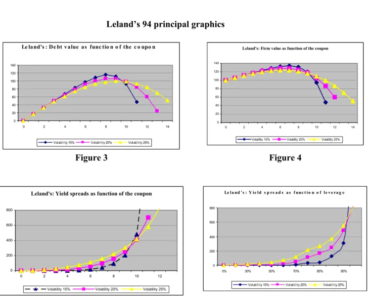
Leland’s 94 principal graphics Le land's : De bt value as func tio n o f the c o upo n
0 20 40 60 80 100 120 140 0 2 4 6 8 10 12 14
Volatility 15% Volatility 20% Volatility 25%
Leland's: Firm value as function of the coupon
0 20 40 60 80 100 120 140 0 2 4 6 8 10 12 14
Volatility 15% Volatility 20% Volatility 25%
Figure 3 Figure 4
Leland's: Yield spreads as function of the coupon
0 200 400 600 800 0 2 4 6 8 10 12
Volatility 15% Volatility 20% Volatility 25%
Le la nd 's : Y ie ld s p re a d s a s f unc t io n o f le v e ra g e 0 200 400 600 800 0% 30% 50% 70% 85% 95%
Volatility 15% Volatility 20% Volatility 25%
Graphics in the double exponential jump diffusion model D e bt v a l ue a s f unc t i on of c oupon a nd v ol a t i l i t y 0 20 40 60 80 100 120 0 2 4 6 7 8 9 10 11 12 13 14 15
Sigma20 Sigma15 Sigma25
Firm value as function of coupon and volatility
0 20 40 60 80 100 120 140 0 2 4 6 7 8 9 10 11 12 13 14
Sigma20 Sigma15 Sigma25
Figure 7 Figure 8
Debt value in fonction of leverage and volatility
0 20 40 60 80 100 120 0% 30% 50% 70% 80% 85% 90% 95% 100%
Sigma=20% Sigma=15% Sigma=25%
Firm value as fonction of leverage and volatility
0 20 40 60 80 100 120 140 0% 30% 50% 70% 80% 85% 90% 95% 100%
Sigma=20% Sigma=15% Sigma=25%
Figure 9 Figure 10
Credit spread as fonction of leverage and volatility
0 100 200 300 400 500 600 700 800 900 1000 0 2 4 6 7 8 9 10 11
Sigma=20% Sigma=15% Sigma=25%
Credit spread as fonction of leverage and volatility
0 200 400 600 800 1000 1200 1400 1600 0% 30% 50% 70% 80% 85% 90% 95% 100%
Sigma=20% Sigma=15% Sigma=25%
Figure 11 Figure 12
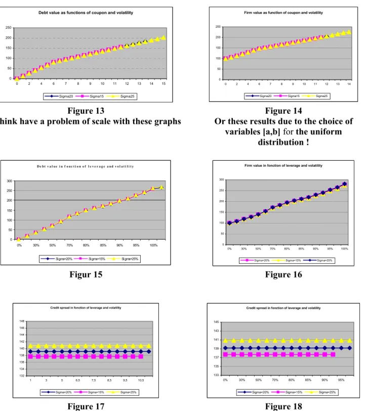
Graphics in the uniform jump diffusion model Debt value as functions of coupon and volatility
0 50 100 150 200 250 0 2 4 6 7 8 9 10 11 12 13 14 15
Sigma20 Sigma15 Sigma25
Firm value as function of coupon and volatility
0 50 100 150 200 250 0 2 4 6 7 8 9 10 11 12 13 14 Sigma20 Sigma15 Sigma25
Figure 13 Figure 14
I think have a problem of scale with these graphs Or these results due to the choice of
variables [a,b] for the uniform distribution ! D e bt v a l ue i n f o nc t i o n o f l e v e r a g e a nd v o l a t i l i t y 0 50 100 150 200 250 300 0% 30% 50% 70% 80% 85% 90% 95% 100%
Sigma=20% Sigma=15% Sigma=25%
Firm value in fonction of leverage and volatility
0 50 100 150 200 250 300 0% 30% 50% 70% 80% 85% 90% 95% 100% Sigma=20% Sigma=15% Sigma=25%
Figur 15 Figure 16
Credit spread in fonction of leverage and volatility
132 134 136 138 140 142 144 146 148 1 3 5 6,5 7,5 8,5 9,5 10,5 Sigma=20% Sigma=15% Sigma=25%
Credit spread in fonction of leverage and volatility
133 135 137 139 141 143 145 0% 30% 50% 70% 80% 85% 90% 95%
Sigma=20% Sigma=15% Sigma=25%
Appendix A:Demonstration of the formula of perpetual American put option in the double exponential jump diffusion model
The demonstration below strongly resembles of the Appendix 1 in Kou and Wang [18]. However, to clarify, we present it here in further detail.
Assumption:
Suppose there exist some xB : exB < K and a non negative function u(x) C1 such that:
1. u (x) is C2 on
<\ {xB} , u (xB−)and u (xB+) existing and u (x) is convex 2. (Lu) (x)− ru (x) = 0 for ∀x ≥ xB 3. (Lu) (x)− ru (x) < 0 for ∀x < xB 4. u (x) > (K− ex)+ for ∀x ≥ xB 5. u (x) = (K− ex)+ for ∀x < xB
and suppose there exists a random variable Z with E [Z] <∞, such that:
e−r(t∧τ ∧τ∗)u(X (t∧ τ ∧ τ∗) + x)≤ Z, ∀t > 0, x, ∀τ
Results:
Then the optimal stopping time is given by τ∗ = inf{t ≥ 0; Vt≤ exB}
And then the value of the perpetual American put option is given by P A(V ) = u (V ) where the value function V is given by
u(x) = ½ K− ex if x < x B Ae−xβ3,r+ Be−xβ4,α if x≥ x B
The infinitesimal generator of the double jump diffusion process is given by Lu(x) = 1 2σ 2u00(x) + µu0(x) + λ Z +∞ −∞ [u (x + y)− u (x)] fY (y) dy
where u (x) is a twice continuously differential function and µ =³r− δ − σ2
2 − λξ ´
.
To compute the quantity (Lu) (x), we need to first calculate the term R+∞
−∞ u(x + y) fY (y) dy
Since the value of u depends on the position with respect to xB, we shall consider two cases.
We first consider the case x≥ xB In that case,
R+∞
−∞ u(x + y)fY(y)dy = RxB−x −∞ (K− e x+y)qη 2eyη2dy +Rx0 B−x(Ae −(x+y)β3 + Be−(x+y)β4)qη 2eyη2dy +R0+∞(Ae−(x+y)β3 + Be−(x+y)β4)pη
1e−yη1dy = I1+ I2 + I3
The quantities Ii are obtained as follows: I1 = η1 2qη2Ke yη2 |xB−x −∞ −1+η12e xqη 2ey(1+η2) | xB−x −∞ = qe(xB−x) h K − η2 1+η2e xBη2 i I2 = (η 1 2−β3)e −β3xqη 2Ae−(η2−β3)y |0xB−x + 1 (η2−β4)e −β4xqη 2Be−(η2−β4)y |0xB−x = η2 (η2−β3)qA £ e−β3x− e−β3xBeη2(xB−x)¤+ η2 (η2−β4)qB £ e−β4x− e−β4xBeη2(xB−x)¤ I3 = −(ηη1 1+β3)e −β3xpAe−(η1+β3)y |∞ 0 + η1 −(η1+β4)e −β4xpBe−(η1+β4)y |∞ 0 = η1 (η1+β3)pAe −β3x+ η1 (η1+β4)pBe −β4x
(Lu) (x)− ru (x) = 12σ2u00(x) + µu0(x) + λR+∞ −∞ [u (x + y)− u (x)] fY (y) dy− ru (x) = 1 2σ 2¡Aβ2 3e−xβ3 + Bβ 2 4e−xβ4 ¢ − µ¡Aβ3e−xβ3 + Bβ 4e−xβ4 ¢ −r¡Ae−xβ3 + Be−xβ4¢− λ¡Ae−xβ3 + Be−xβ4¢ +λ qe(xB−x) h K− η2 1+η2e xBη2 i + η2 (η2−β3)qA £ e−β3x− e−β3xBeη2(xB−x)¤ + η2 (η2−β4)qB £ e−β4x− e−β4xBeη2(xB−x)¤ + η1 (η1+β3)pAe −β3x+ η1 (η1+β4)pBe −β4x
recall the function G (x) is:
G(x) = 1 2σ 2 x2+ µx + λ µ pη1 η1 − x + qη2 η2 + x − 1 ¶ we can pose f(x) = G (−x) − r = 1 2σ 2x2 − µx + λ µ pη1 η1 + x+ qη2 η2 − x− 1 
then we have (Lu) (x)− ru (x) (Lu) (x)− ru (x) = Ae−xβ3f(β 3) + Be−xβ4f(β4) +λqe(xB−x)η2 h K− η2 1+η2e xB − η2 η2−β3Ae −β3xB − η2 η2−β4Be −β4xB i
As −β3,−β4 are roots of G (β) = r so f (β3) = 0 and f (β4) = 0 We can deduce that (Lu) (x)− ru (x) = 0 implies
· K − η2 1 + η2e xB − η η2 2 − β3 Ae−β3xB − η η2 2− β4 Be−β4xB ¸ = 0
We have three unknowns exB, A, B so we need three equations in
order to solve these unknowns.
When we recall the function u (x) at xB, we have the first equation: K− exB = Ae−xBβ3 + Be−xBβ4
The smooth fit condition4 at xB gives us the second equation:
4The validation of smooth fit condition can be found in Boyarchenko and
exB = Aβ
3e−xB
β3 + Bβ
4e−xB β4
And the third equation, we have from (Lu) (x)− ru (x) = 0: · K − η2 1 + η2e xB − η η2 2 − β3 Ae−β3xB − η η2 2− β4 Be−β4xB ¸ = 0 From the first and second equation, we have the formulas of A and B: A=−β4K − e xBβ 4− exB (β3− β4) e−β3xB B = −e xB + β 3K− β3exB (β3− β4) e−β4xB
Inserting the values of A and B into the third equation generates these formulas: A= exBβ3 1 + β4 β4− β3 µ β4 1 + β4K− e xB ¶ (16) B = eβ4xB 1 + β3 β4− β3 µ exB − 1 + ββ3 3 K ¶ exB = Kη2+ 1 η2 β3 1 + β3 β4 1 + β4 So we have proven the condition n◦2.
The conditions n◦1, 4, 5 follow easily as we have u (xB+) = u (xB−) and 0≤ u (x) ≤ K
The only remaining condition that we have to prove is the condition n◦3. That is in the case x < x
B. In that case: R+∞ −∞ u(x + y) fY (y) dy = R0 −∞(K− e x+y) qη 2eyη2dy +RxB−x 0 (K− e x+y) pη 1e−yη1dy +Rx+∞ B−x ¡ Ae−(x+y)β3 + Be−(x+y)β4¢pη 1e−yη1dy = II1+ II2+ II3
The quantities IIi are obtained as follows: II1 = η2 η2qKe yη2 |0 −∞− η2 1+η2e xqey(1+η2)|0 −∞ = Kq− η2 1+η2e xq II2 =− η1 η1pKe −yη1 |xB−x 0 − η1 (η1−1)pe xe−y(1+η1) |xB−x 0 = pK− pKe−η1(xB−x)− η1 (η1−1)pe x+ η1 (η1−1)pe xBe−η1(xB−x) II3 = η1 −(η1+β3)e −β3xpAe−(η1+β3)y |∞ xB−x + η1 −(η1+β4)e −β4ypBe−(η1+β4)y |∞ xB−x = η1 (η1+β3)e −β3xBpAe−η1(xB−x)+ η1 (η1+β4)e −β4xBpBe−η1(xB−x)
To arrange the terms of the quantities IIi, we have:
II1+ II2+ II3 = K− ex h pη 1 η1−1 + qη2 1+η2 i −pe−η1(xB−x) h K− η1 1−1e xB − η1 η1+β3Ae −β3xB − η1 η1+β4Be −β4xB i
We can now compute (Lu) (x)− ru (x) in this case of x < xB :
(Lu) (x)− ru (x) = 12σ2u00(x) + µu0(x) + λR−∞+∞[u (x + y)− u (x)] fY (y) dy− ru (x)
= 12σ2ex− µex− r (K − ex)− λ (K − ex) +λ K− e xh pη1 η1−1 + qη2 1+η2 i −pe−η1(xB−x) h K−η 1 1−1e xB − η1 η1+β3Ae −β3xB − η1 η1+β4Be −β4xB i We have ξ = pη1 η 1−1 + qη2 η 2+1 and µ = ¡r− δ − 12σ2 − λξ¢. Then (Lu) (x)− ru(x) is equal ⇐⇒ −rK+δex−λpe−η1(xB−x) · K− 1 η1− 1e xB − η η1 1+ β3 Ae−β3xB − η η1 1+ β4 Be−β4xB ¸
K− η1 1−1e xB − η1 η1+β3Ae −β3xB − η1 η1+β4Be −β4xB = K− η1 1−1e xB − η1 η1+β3 1+β4 β4−β3 ³ β 4 1+β4K − e xB ´ − η1 η1+β4 1+β3 β4−β3 ³ exB − β3 1+β3K ´
We can also rearrange the equation above with terms exB and K
= exB ³ −η11−1 + η1 η1+β3 1+β4 β4−β3 + η1 η1+β4 1+β3 β4−β3 ´ +K³1− η1 η1+β3 β4 β4−β3 + η1 η1+β4 β3 β4−β3 ´
Replacing exB with its value as in (16) generates:
= Kη2+1 η2 β3 1+β3 β4 1+β4 ³ −β3β4η1 (η1−1)(η1+β3)(η1+β4) ´ +K β3 η1+β3 β4 η1+β4 = −K β3 η1+β3 β4 η1+β4 η2+η1 η2(η1−1)
Then, we can generate the reduced form of (Lu) (x)− ru (x) which is:
(Lu) (x)−ru (x) = −rK+δex+λpe−η1(xB−x)K β3
η1+ β3 β4 η1+ β4
η2+ η1 η2(η1− 1) ≤ 0 So the condition N o3 is proven.
–––––––—
Appendix B: Demonstration of the formula of perpetual American put option in the uniform jump diffusion case.
References
[1] Bates (1996), ”Jumps and Stochastic Volatility: Exchange Rate Process Implicit in Deutsche Mark Option”, Review of Financial Studies, Vol.9, No.1, p.69-107
[2] Bertoin, J. (1996), ”Some elements on L´evy processes”, Cambridge University press, Cambridge.
[3] Black, F., Myron Scholes, (1973), ”The Pricing of Options and Cor-porate Liabilities”, Journal of Politicial Economy, Vol. 81, iss.3, p.637-653.
[4] Boyarchenko, S. (2000), ”Endogenous default under L´evy process”, Working Paper, University of Pennsylvania, p.1-16.
[5] Boyarchenko, S., S. Levendorskii, (2002) ”Non-Gaussian Merton-Black-Scholes Theory: Preface and Contents”, Vol.9, New Jersey-London-Singapore-HongKong, World Scientific, 398p.
[6] Boyarchenko, S., S. Levendorskii, (2000), ”Barrier options and touch-and-out options under regular Levy processes of exponential type”, Working paper, No.45, MaPhySto, Aarhus University. [7] Boyarchenko, S., S. Levendorskii, (2001), ”Option pricing and
hedging under regular Levy processes of exponential type”, in M. Kohlmann and S. Tang (eds.), Mathematical Finance, p.121-130. [8] Boyarchenko, S., S. Levendorskii, (2000), ”Option pricing for
trun-cated Levy processes”, International Journal of Theoretical and Ap-plied Finance, Vol.3, p.549-552.
[9] Carr, Geman, Madan, Yor, (2001), ”Time Changes for L´evy Pro-cesses”, Mathematical Finance, 2001.
[10] Carr, Geman, Madan, Yor, (2003), ”Stochastic Volatility for Levy processes”, Mathematical Finance, 2003.
[11] Ericsson, J. (2000), ”Asset substitution, debt pricing, optimal lever-age and maturity”, Finance, vol. 21, p.39-70.
[12] Ericsson, J., Joel Reneby, (1998), ”A framework for valuing corpo-rate securities”, Applied Mathematical Finance, iss.5, p.143-163. [13] Gukhal, C.R.,(2001), ”Analytical Valuation of American Options
on Jump-Diffusion Processes”, Mathematical Finance, Vol 11, No.1, p.97-115.
[14] Jeanblanc, M., Marek Rutkowski, (2000), ”Modelling of Default Risk: Mathematical Tools”, Working Paper, Evry University. [15] Hilberink, B., Chris L.G. Rogers, (2000), ”Optimal capital structure
and endogenous default”, Working papers - University of Bath, p.1-30.
[16] Kou S. G. (2002), ”A jump diffusion model for option pricing”. Management Science. vol. 48, p.1086-1101.
diffusion process”. Advances in Applied Probability, Vol. 35, 504-531.
[18] Kou S. C. and H. Wang, (2001) ”Option Pricing under a Dou-ble Exponential Jump Diffusion Model”, Working Paper, Columbia University, p.1-21.
[19] Leland, H.E. (1994), ”Corporate debt value, bonds covenants and optimal capital structure”, The Journal of Finance, vol. 49, iss.4, p.1213-1253.
[20] Leland, H.E., Klauss Bjerre Toft, (1996), ”Optimal Capital Struc-ture, Endogenous Bankruptcy, and the Term Structure of Credit Spreads”, The Journal of Finance, vol. 51, iss.3, p.987-1019.
[21] Merton, R. (1974), ”On the Pricing of Corporate Debt : the Risk Structure of Interest Rates”, Journal of Finance, vol. 29, iss.2, June, p.449-470.
[22] Merton, R. (1976), ”Option Pricing when the underlying stock re-turns are discontinuous”, Journal of Financial Economics, vol. 3, p.125-144.
[23] Mordecki, E. (1997), ”Optimal Stopping for a Compound Poisson Process with Exponential Jumps”, Publicaciones Matem´aticas del Uruguay. Vol. 7, p.55-66.
[24] Mordecki, E. (1997), ”Ruin probabilities and optimal stopping for a diffusion with jumps”, Proceedings of the Fourth Congress ”Dr. Antonio A. R. Monteiro” (Bahia Blanca, p.39-48.
[25] Mordecki, E. (2002), ”Optimal stopping and perpetual options for L´evy processes”, Finance and Stochastics, Volume VI, iss.4, p.473-493.
[26] Mordecki, E. (2002), ”Perpetual Options for L´evy Processes in the Bachelier Model”, Proceedings of the Steklov Mathematical Insti-tute, Vol. 237, p. 256-264.
[27] Ozkan, F. (2002), ”Levy Processes in Credit Risk and Market Mod-els”, Doctoral Thesis, University of Feiburg.
[28] Ozkan, F., E., Eberlein (2003), ”Defaultable L´evy term structure: ratings and restructuring”, Mathematical Finance, p.277-300. [29] Zhou, C. (1997), ”A Jump-Diffusion Approach to Modeling Credit
Risk and Valuing Defaultable Securities”, Working paper, Wash-ington, DC: Federal Reserve Board.