First steps towards an advanced simulation of composites manufacturing by automated tape placement

HAL Id: hal-01763316

https://hal.archives-ouvertes.fr/hal-01763316

Submitted on 10 Apr 2018

HAL is a multi-disciplinary open access archive for the deposit and dissemination of sci-entific research documents, whether they are pub-lished or not. The documents may come from teaching and research institutions in France or abroad, or from public or private research centers.

L’archive ouverte pluridisciplinaire HAL, est destinée au dépôt et à la diffusion de documents scientifiques de niveau recherche, publiés ou non, émanant des établissements d’enseignement et de recherche français ou étrangers, des laboratoires publics ou privés.

First steps towards an advanced simulation of

composites manufacturing by automated tape placement

Francisco Chinesta, Adrien Leygue, Brice Bognet, Chady Ghnatios, Fabien

Poulhaon, Felipe Bordeu, Anaïs Barasinski, Arnaud Poitou, Sylvain Chatel,

Serge Maison-Le Poëc

To cite this version:

Francisco Chinesta, Adrien Leygue, Brice Bognet, Chady Ghnatios, Fabien Poulhaon, et al.. First steps towards an advanced simulation of composites manufacturing by automated tape placement. International Journal of Material Forming, Springer Verlag, 2014, 7 (1), pp.81-92. �10.1007/s12289-012-1112-9�. �hal-01763316�

FIRST STEPS TOWARDS AN ADVANCED SIMULATION OF

COMPOSITES MAUFACTURING BY AUTOMATED TAPE

PLACEMENT

F. Chinesta1, A. Leygue1, B. Bognet1, Ch. Ghnatios1, F. Poulhaon1, F. Bordeu1, A.

Barasinski1, A. Poitou1, S. Chatel2 & S. Maison-Le-Poec2

1 _{EADS Chair, GeM Institute, Ecole Centrale de Nantes} 1 rue de la Noe, F-44321 Nantes cedex 3, France

Francisco.Chinesta@ec-nantes.fr

2 _{EADS-IW, Rue Belouga, 44300 Bouguenais, France}

Sylvain.Chatel@eads.net

Abstract

Composite materials and their related manufacturing processes involve many modeling and simulation issues, mainly related to their multi-physics and multi-scale nature, to the strong couplings and the complex geometries. In our former works we developed a new paradigm for addressing the solution of such complex models, the so-called Proper Generalized Decomposition based model order reduction. In this work we are summarizing the most outstanding capabilities of such methodology and then all these capabilities will be put together for addressing efficiently the simulation of a challenging composites manufacturing process, the automated tape placement.

Keywords: composites; automated tape placement; numerical simulation; model order

reduction; PGD.

1. Introduction

The production of large pieces made of thermoplastic composites is a challenging issue for today’s industry. Thermoplastic composites still represents a niche market because of the difficulties associated to their processing. Several reliable manufacturing processes are now available for building-up thermoplastic laminated structures. Among them, the automated tape placement (ATP) appears to be an appealing process. In this process a tape is placed and progressively welded on the substrate consisting in the tapes previously placed. By laying additional layers in different directions, a part with desired properties and geometry can be produced. However, the welding of two thermoplastic layers requires specific physical conditions: a permanent contact, also

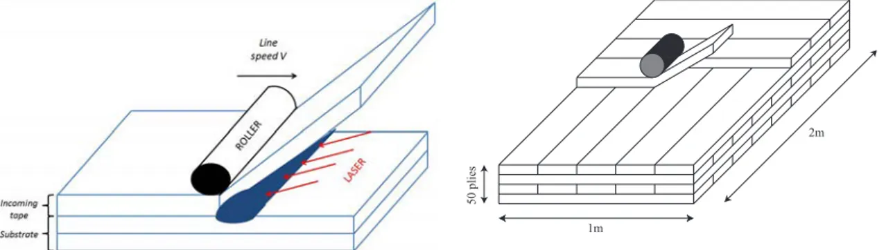
called intimate contact, and a temperature that has to be high enough during a time large enough to ensure the diffusion of macromolecules, without significant material degradation. Due to the low thermal conductivity of thermoplastics, a high temperature at the interface can be reached with a local heating. ATP uses a laser (or sometimes hot gas torches) and a cylindrical consolidation roller to ensure both conditions required for the proper welding, as depicted on Fig. 1.

Figure 1. Sketch of automated tape placement

The numerical simulation of such a process is the subject on an intensive research work. Indeed, because of the successive heating and cooling of the structure during the addition of new tapes, residual stresses appear in the formed part. The evaluation of these residual stresses is crucial because they have a significant impact on both the mechanical properties and the geometry of the manufactured plate or shell due to the springback. They can in particular lead to a distortion of the part, inter-ply delamination or matrix cracking. High-levels of stress may arise because of two reasons. First, the large differences in the thermal expansion coefficients of the matrix and the fibers lead to an important deformation at the matrix/fiber interface. Stresses also appear when two consecutive plies do not have the same reinforcement orientations. In that case, the different thermal expansion coefficients induce again stresses at the plies interfaces. Experimentally, it is quite difficult to measure residual stresses. Destructive methods use the release of stress and its associated strain when performing a cutting of the structure. Non-destructive methods like X-ray diffraction or neutron diffraction are more accurate but still very expensive. The numerical simulation turns out therefore to be one of the cheapest and most promising alternative to model and optimize such processes but several issues related to the process itself make the task quite complicated as we are going to expose throughout this work.

Several models were proposed since the early 90's. We can mention in particular the numerical analysis made by Sonnez et al. [1] and the work by Pitchumani et al. [2]

!"

#"

$%

interested in the study of interfacial bonding. In the latter, the domain considered is only 2D and strong assumptions were introduced in the thermal model, in particular concerning the boundary conditions. Moreover, in order to simplify the geometry of the domain, an incoming tow was assumed instantaneously laid down all along the substrate, which is far from being the case in the real process. Finally, the thermal/mechanical contact was assumed to be perfect at the inter-ply interfaces, which again seems to be also a crude assumption. First attempts of the modeling and simulations of this process can be found in [3,4].

In what follows the domain we consider is 3D and the material, the carbon reinforced PolyEther Ether Ketone (PEEK), is anisotropic. The thermal and mechanical properties of this material are detailed in Tables 1 and 2. In these tables, the index 1 refers to the longitudinal or fiber direction, the index 2 corresponds to the transverse direction and the index 3 stands for the ''through the thickness'' direction.

Thermal diffusivity (10-6 m2/s) K11=1.89 K22=0.189 K33=0.189

Thermal expansion (10-6 /°K) α11=0.2 α22=60 α33=60

Table 1. Thermal properties of carbon reinforced PEEK (AS4/APC2)

Young modulus (GPa) E11=137 E22=9.4 E33=9.1

Poisson ratio ν12=0.33 ν13=0.32 ν23=0.40

Shear modulus (GPa) G12=5.1 G13=4.7 G23=3.2

Table 2. Mechanical properties of carbon reinforced PEEK (AS4/APC2)

In this work we propose some improvements to existing models. First of all, the domain we consider is 3D and the material anisotropic. In order to take into account the imperfect adhesion at the inter-ply interface, thermal contact resistances are introduced. Regarding the mechanical problem, the incoming tow is progressively laid down on the substrate and is subjected to a tension force in order to reproduce the pre-tension applied in the real process. But actually, beyond the model itself, the numerical method employed for the solution of the thermal and mechanical problems associated to the ATP process is novel. This work represents a first step towards a global thermo-mechanical process modeling using robust and efficient numerical tools. The numerical

strategy we propose is based on the Proper Generalized Decomposition (PGD) [5,6]. This method uses a separated representation of the unknown field, in that case temperature or displacements, and results in a tremendous reduction of the computational complexity of the model solution. Moreover, it entails the ability to introduce any type of parameters (geometrical, material …) as extra-coordinates into the model, to obtain by solving only once the resulting multidimensional model the whole envelope containing all possible solutions [7,8], a sort of numerical virtual chart or metamodel, that can be then exploited on-line even on light computing platforms like smartphones of tablets [9,10].

2. Building-up parametric solution

In what follows we are illustrating the construction of the Proper Generalized Decomposition by considering a quite simple problem, the parametric heat transfer equation governing the evolution of u(x,t, k):

∂u

∂t − kΔu − f = 0 (1)

where (x,t,k) ∈Ω × I × ℑ and for the sake of simplicity the source term is assumed constant, i.e. f = cst . Because we are interested in knowing the temperature field u(x,t)

for any value of the thermal conductivity k∈ℑ, the conductivity will be assumed as a

new coordinate, like space x or time t . Thus, instead of solving the thermal model for different values of the conductivity parameter we prefer introducing it as a new coordinate looking directly for u(x,t,k) . The price to be paid is the increase of the model dimensionality; however, as the complexity of the PGD scales linearly with the space dimension the introduction of the conductivity as a new coordinate allows for faster and cheaper solutions.

Within the PGD framework the solution of Eq. (1) is searched under the separated form:

u x,t,k

( )

≈ X_i

( )

x

i=1

i= N

∑

⋅T_i

( )

t ⋅ K_i

( )

k (2)

In what follows we are assuming that the approximation at iteration n is already known:

un

( )

_{x,t,k = X} i

( )

x i=1 i= n

∑

⋅T_i

( )

t ⋅ K_i

( )

k (3)

and at present iteration we look for the next functional product Xn+1

( )

x ⋅Tn+1

( )

t ⋅ Kn+1

( )

k that for alleviating the notation will be denoted by

. In order to solve the resulting non-linear problem, some linearization strategy is compulsory. The simplest choice consists in using an alternating

directions fixed-point algorithm. It proceeds by assuming and given at the

previous iteration of the non-linear solver and then computing . From the just

updated and we can update , and finally from the just computed

and we compute . The procedure continues until reaching

convergence. The converged functions , and allow defining the

searched functions:

Xn+1

( )

x = R x

( )

, Tn+1

( )

t = S t

( )

and Kn+1

( )

k = W k

( )

and then we

can move to the next enrichment. The interested reader can refer to [9,10] and the references therein for additional details on the PGD constructor.

3. ATP thermal model

Our objective is to obtain the steady state temperature in a coordinate system attached to the placement head, which is assumed to move with a constant velocity. For a given number of plies, this temperature field can be used to reconstruct the thermal history in

any material point far enough from the edges, as will be illustrated later. In these

conditions each material point experiences the same thermal history during the process. It is progressively heated when approaching the laser, it reaches its maximum temperature when the laser applies directly on it and it cools down relatively fast when getting far from the heat source, reaching the ambient temperature before the laser comes back again when placing the next layer. Therefore, instead of considering a problem where the domain is fixed and the boundary conditions are time dependent, we

can explicitly introduce the line speed v= (v,0,0) (when the heating device moves in

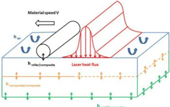
the x -direction) in the heat transfer equation by adding a convection term. In other words, the laser and the roller are kept fixed and the material is assumed moving with a speed v in the opposite direction to the one in which laser and roller move, as shown on Fig. 2. In this figure we have emphasized the fact that after applying the heat source the incoming layer adheres to the substrate (continuous line), being this adhesion more or less perfect depending on the molecular diffusion as discussed later. On the other hand, before experiencing the bonding the interface between the incoming layer and the substrate, represented by a broken line in Fig. 2, is assumed adiabatic, that is, the incoming layer and the substrate cannot exchange heat trough it.

Figure 2. Thermal model

Hence the equation to be solved writes

ρ ⋅Cp⋅ v ⋅∇T = ∇ ⋅ K ⋅∇T

(

)

(4)

where ρ is the density, Cp is the specific heat and K is the conductivity tensor. In this

reference frame, the boundary conditions are not time dependent anymore. The solution of Eq. (4) corresponds to the steady state temperature field in the coordinate system attached to the roller and the laser. The material domain, consisting of the substrate (plies already placed) and the incoming layer, in which equation (4) is solved is noted by Ω = 0, L

[

x

]

× 0, L⎡⎣ y⎤⎦ × 0,L⎡⎣ z⎤⎦ .

The incoming ply and the substrate are assumed having the ambient temperature. Thus, on the upstream boundary the ambient temperature will be enforced and on the downstream boundary the heat flux is assumed vanishing. Convection boundary conditions are enforced on the upper surface, except in the regions in which the laser and the roller apply and finally a conduction transmission condition is enforced in the contact between the composite and the work plane. All the transmission conditions (at the inter-plies, at the roller-composite contact and on the composite-work-plane

interface) are affected by a contact thermal resistance h accounting for the non-perfect

contacts. These resistances depend on the applied pressure and also on the inter-plies bonding. Thus, the temperature field becomes discontinuous at the plies interfaces and also on the composite-work-plane and roller-composite contacts. On the interface between the incoming ply and the substrate that has not already experienced the molecular bonding (broken line in Fig. 2) an infinite value of the contact thermal resistance is assumed ensuring the absence of heat transfer between the incoming ply and the substrate. As soon as the bonding occurs (continuous line in Fig. 2) a thermal resistance applies, whose value depends on the quality of such bonding, vanishing when

the adhesion can be considered perfect. A parameter quantifying the quality of the bonding will be introduced later.

As the different contact thermal resistances are unknown “a priori” they should be identified from experiments by solving the corresponding inverse problem, that is, looking for the values of the different contact thermal resistances allowing reproducing the experimental measurements. In order to perform this identification we must define a cost function to be minimized by assuming any optimization strategy. The natural choice for such a cost function is the gap between the computed temperatures at some locations and the temperature measured at such positions. The main drawback is that for each tentative choice of the different thermal resistances Eq. (4) must be solved, the cost function evaluated and if its value is not small enough, the value of the thermal resistances must be updated trying to minimize the cost function, that is the gaps, and then the thermal model (4) must be solved again, and so on until reaching a value of the cost function small enough allowing to fix the value of the thermal resistances to be considered from now on in the thermal model of the process.

In order to solve a single problem instead of one for each choice of the thermal resistances, one could imagine introducing the thermal resistances as extra-coordinates into the thermal model. We distinguish three thermal resistances, the one related to the contact between the roller and the laminate, the one applying at the inter-plies interfaces and finally the one existing between the laminate and the work-plane. The inverse of

three resistances will be denoted by h1, h2 and h3. Thus, we could imagine that the best

representation of the temperature field in the roller-laser frame consists of

T (x, h1, h2, h3) . Such a representation has as main drawback the fact to be defined in a

space of dimension 6, the three space coordinates and the three extra-coordinates representing the contact resistances. The difficulties related to the model’s multi-dimensionality can be circumvented thanks to the separated representation involved by the PGD constructor that writes:

T x,h

(

₁,h₂,h₃

)

≈ X_i

( )

x i=1 i= N

∑

⋅ H_i1 _h 1

( )

⋅ H_i2 _h 2

( )

⋅ H_i3 _h 3

( )

= X_i

( )

x i=1 i= N

∑

⋅ H_ij _h j

( )

j=1 j=3

∏

(5)

whose solution involves the solution of a sequence of 3D problems (of the order of N )

related to the computation of functions Xi

( )

x and the same number multiplied by 3 of

one-dimensional problems for computing functions Hi 1 _h 1

( )

, Hi 2 _h 2

( )

and Hi 3 _h 3

( )

. Because the computing time for solving the local one-dimensional problems can be

neglected with respect to the one needed for solving the 3D problems, we can conclude that the complexity associated with the 6D solution (5) scales with the one related to the solution of a standard 3D steady state thermal problem.

Obviously, if the number of iterations required for minimizing the gap in the inverse identification is of the same order as N there is no apparent benefit in computing the parametric solution (5). However, there is a noticeable benefit that we are trying to highlight. As soon as the process parameters change (laser power, line velocity or roller pressure) the contact resistances will change, and they should be identified again, by solving again many 3D problems for attaining an acceptable value of the temperature gap at the locations where the temperature is measured. Thus, each choice of the process parameters will imply a new inverse analysis and then the solution of many direct problems. One could imagine that by computing the parametric solution (5) a single calculation suffices, but this is not totally true. For computing a general enough parametric solution encompassing any choice of the process parameters and the contact thermal resistances, the process parameters should be also included as extra-coordinates.

If we denote by p the laser power, by v , as previously used, the line velocity, and

neglecting in first approximation the influence of the roller contact pressure, the

parametric temperature writes T (x,h1, h2h3, p, v) . It can be searched under the separated

form: T x,h

(

₁,h₂,h₃, p,v

)

≈ X_i

( )

x i=1 i= N

∑

⋅ H_i1 _h 1

( )

⋅ H_i2 _h 2

( )

⋅ H_i3 _h 3

( )

⋅ P_i

( )

p ⋅V_i

( )

v (6) with a moderate impact on the computational complexity because the two new coordinates only involve the solution of some local one-dimensional problems within the PGD constructor methodology. It must be noticed that the solution (6) is calculated off-line, and then particularized on-line in the process simulation or within the inverse identification procedure.

Moreover, because the hexahedral geometry of the tape, one could prefer performing a full space decomposition by writing the approximation (7) instead of (6):

T x, y, z,h

(

₁,h₂,h₃, p,v

)

≈ ≈ X_i

( )

x i=1 i= N

∑

⋅Y_i

( )

y ⋅ Z_i

( )

z ⋅ H_i1 _h 1

( )

⋅ H_i2 _h 2

( )

⋅ H_i3 _h 3

( )

⋅ P_i

( )

p ⋅V_i

( )

v (7)

that only involves the solution of a sequence of one-dimensional problems, some of them, the ones concerning the space functions X_i

( )

x , Y_i

( )

y and Z_i

( )

z , defining

standard boundary value problems –BVP- and the ones related to all the extra-coordinates defining local one-dimensional problems that do not need the solution of any linear system of equations, allowing consequently very fast calculations. Other intermediate alternatives exist. The one we will consider later in this work consists of

the in-plane-out-of-plane separated representation in which the coordinates x, y

( )

are

separated from the one related to the laminate thickness z

( )

in the approximation of

functions of space.

The solution (7) is computed off-line for a given tape geometry and the material thermal

parameters ρ , C_{p and the components of the thermal conductivity K . All these}

parameters could be also included as extra-coordinates, but that in the simulation below were not. Then the solution (7) is particularized for obtaining the temperature field for any choice of the process parameters T (x;h1, h2h3, p, v) . This particularization can be

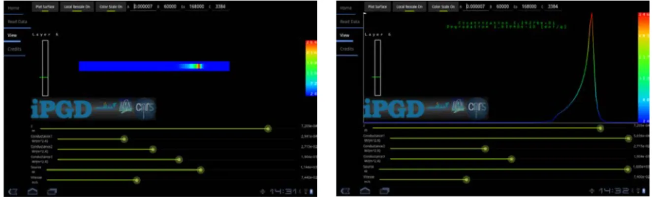
performed on-line, in real time and even on light computation platforms like smartphones or tablets. Fig. 3 depicts one application on a tablet in which the process parameters (the three contact resistances, the line velocity and the laser power) can be selected from the sliders, visualizing in real time the resulting temperature field.

Figure 3. Particularizing online on a tablet the general parametric thermal solution Obviously such a numerical tool has numerous interests. First of all it allows identifying contact thermal resistances such that the numerical solution fits at the best experimental measurements. Moreover, as soon as the thermal history is known we can evaluate both the inter-plies bonding and the material degradation. The first can be calculated by defining an indicator C taking into account the molecular reptation, as was proposed in [11]: C(M,t)= dτ t_r

(

T (M,τ )

)

0 t

∫

(8)

where M represents a material point located at the plies interface and tr is the reptation time that depends on the temperature and that represents the time required for a molecule to escape from its initial tube (the one existing before the beginning of the

thermal process at time t _{= 0 ) at a certain temperature. This time can be characterized}

for each material experimentally and in general follows an Arrhenius’s law. We can

notice that C M,t

(

)

≥ 1 implies a perfect bonding that ensures that the properties at the

interface and the ones of the bulk are the same when neglecting interface porosity. The kinetics (8) is local and can therefore be calculated on-line. The only tricky point is the relation between points x in the thermal model (4), considered in the laser-roller frame, and the material point M . We come back to this issue later. Now, we are focusing in the other phenomenon, the one related to the material degradation due to thermal induced molecular breaking. Following again [11] we consider the damage indicator D given by the kinetics:

D(M,t)= d T(M,τ )

(

)

⋅ dτ

0

t

∫

(9)

where again the temperature dependent damage function

d T (M,

(

τ )

)

follows an Arrhenius’s law that can be for each material easily identified experimentally.

We come back to the question concerning the relation between T x

( )

coming from the

solution of Eq. (4) and T M,τ

(

)

. We consider the situation depicted in Fig. 5 (bottom

schema). First of all, we are discussing the value of length of the domain of study Lx.

This value should be compatible with the boundary conditions enforced on the

boundaries x= 0 and x = Lx: the ambient temperature at x= Lx, i.e. T x

(

= Lx

)

= Tamb

and a null heat flux at x= 0 . Thus referring to Fig. 5 (bottom schema) the length must

ensure that the resulting heat flux x= Lx vanishes, i.e.

∂T ∂x x= L_x

≈ 0 , and that at x = 0

the temperature approach again the ambient temperature, i.e. T x

(

= 0

)

≈ Tamb. Now,

with the dimensions of the representative domain defined, we can notice by comparing the real process depicted in the upper scheme of Fig. 5 with the steady state analysis performed in the laser-roller frame (bottom schema), that:

T M,t

( )

₁ = T x

( )

₁ T M,t

( )

₂ = T x

( )

₂ ! T M,t

(

_M

)

= T x

( )

_M ! " # ## $ # # # (10)

result that can be generalized as follows:

T M,t

( )

= T x

(

1! v "t

)

(11)

Thus, from the solution of the steady state model (4) we can easily determine the thermal history of any material point, allowing the computation of the accumulated bonding or damage.

Figure 5. Relation between moving and fixed frames

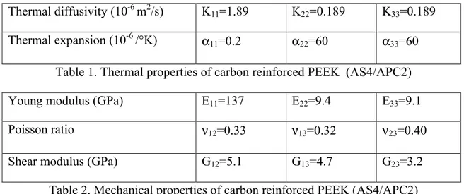
However, the thermal model presented until now is not fully satisfactory despite its richness because as soon as the sequence of plies change, the thermal model must be solved again because the thermal conductivities are changing throughout the thickness. As it can be noticed in Fig. 1 (right) the orientation of the reinforcement could change from one ply to the subsequent. Thus, if for example we are interested in pre-computing all the possible stacking sequences, with 4 possible orientations and 10 plies the number

of possible configurations reaches 410

! 106_{, even when considering all the other}

process parameters (line velocity, laser power and all the contact thermal resistances) given and fixed. By considering that the solution of the thermal model (4) for each

configuration requires one minute, the calculation of all possible laminates ( ! 106₎

needs 2 years of computation. Moreover, after computing this million of solutions they must be stored in order to be used online when needed. It is obvious that such a storage of information is a tricky point, and some kind of data compression procedure seems

compulsory in order to obtain a useful virtual chart or metamodel to be considered efficiently for online purposes (identification, process control …).

In order to calculate a more general parametric solution the orientation of the reinforcement of each ply through the thickness should be added as new extra-coordinates [10]. Doing so, we obtain a solution valid for any orientation sequencing. The separated representation related to the PGD allows circumventing the resulting

curse of dimensionality. If we denote by θ_j the orientation of ply number j , the

separated representation of the temperature field including these new conformational

extra-coordinates θ_j reads: T x, y, z,h₁,h₂,h₃, p,v,θ₁,,θ_N p

(

)

≈ ≈ X_i

( )

x i=1 i= N

∑

⋅Y_i

( )

y ⋅ Z_i

( )

z ⋅ H_i1 _h 1

( )

⋅ H_i2 _h 2

( )

⋅ H_i3 _h 3

( )

⋅ P_i

( )

p ⋅V_i

( )

v ⋅ Θ_ij _θ j

( )

j=1 j= Np

∏

(12)

where N_p denotes the number of plies in the considered laminate.

Now, after these developments regarding the thermal aspects we can move one step forward in order to determine the residual stresses induced distortions of the conformed part due to springback. We start describing the solution procedure of the mechanical problem defined in a plate-like domain, before considering in the last section of the present paper the calculations of the residual stresses installed in the part by solving a more complex thermoelastic model.

4. Mechanical structural analysis

When computing elastic responses of plates, two dimensional plate theories are usually preferred to the numerically expensive solution of the full three-dimensional elastic problem. Going from a 3D elastic problem to a 2D plate theory model usually involves some kinematical and mechanical hypotheses on the evolution of the solution through the thickness of the plate.

Despite the quality of existing plate theories, their solution close to the plate edges is usually wrong as the displacement fields are truly 3D in those regions and do not satisfy the kinematic hypothesis. Moreover, kinematic hypothesis fail where Saint-Venant's principle does not apply. It is well known that some heterogeneous complex plates do not verify the Saint Venant's principle anywhere. In that case the solution of the three-dimensional model is mandatory even if its computational complexity could be out of nowadays calculation capabilities.

Most commercial codes for structural mechanics calculations propose different type of plate and shell finite elements, even in the case of multilayered composites plates or shells. However, in composites manufacturing processes the physics encountered in such multilayered plate or shell domains is much richer, because it usually involves chemical reactions, crystallization and strongly coupled non-linear thermo-mechanical behaviors. The complexity of the involved physics makes impossible the introduction of pertinent assumptions for reducing a priori the dimensionality of the model from 3D to 2D. In that case a fully 3D modeling is compulsory, and because of the richness of the thickness description (many coupled physics and many plies with different physical states and directions of anisotropy) the approximation of the fields involved in the models needs thousands of nodes distributed along the thickness direction. Thus, fully 3D descriptions may involve millions of degrees of freedom that should be solved many times because of the history dependent thermo-mechanical behavior. Moreover, when we are considering optimization or inverse identification, many direct problems have to be solved in order to reach the minimum of a certain cost function.

Even if in what follows we are only addressing thermo-elastic behaviors in quite simple configurations whose behavior could be captured accurately by using existing plate models, we prefer to address a new approach that having the same computational complexity as plate models, calculates the real 3D fields. The main ideas of this numerical technique that was described in detail in [10], are here summarized and then applied to calculate the residual stresses induced springback of some ATP laminates.

When we consider the elastic behaviour defined in a plate-like domain Ξ , it suffices

considering an in-plane-out-of-plane separated representation of each component of the displacement vector: u x, y, z

(

)

= u x, y, z

(

)

v x, y, z

(

)

w x, y, z

(

)

⎛ ⎝ ⎜ ⎜ ⎜ ⎜ ⎞ ⎠ ⎟ ⎟ ⎟ ⎟ ≈ u_xyi

( )

_{x, y ⋅u} z i

( )

_z v_xyi

( )

_{x, y ⋅ v} z i

( )

_z w_xyi

( )

_{x, y ⋅ w} z i

( )

_z ⎛ ⎝ ⎜ ⎜ ⎜ ⎜ ⎞ ⎠ ⎟ ⎟ ⎟ ⎟ i=1 i= N

∑

(13)

where

( )

x, y ∈Ω ⊂ ℜ2 and z∈I ⊂ ℜ.

In order to highlight the interest of such a decomposition we are comparing the complexity of PGD-based solvers with respect to the standard finite element method. For the sake of simplicity we will consider a hexahedral domain discretized using a

respectively. Even if the domain thickness is much lower than the other characteristic in-plane dimensions, the physics in the thickness direction could be quite rich, mainly when we consider composites plates composed of hundreds of anisotropic plies in which the complex physics involved requires fully 3D descriptions. In that case thousands of nodes in the thickness direction could be required to represent accurately the solution behaviour in that direction. In usual mesh-based discretization strategies this fact induces a challenging issue because the number of nodes involved in the model

scales with N_x× N_y × N_z, however, if one applies a PGD based discretization, and the

separated representation of the solution involves modes (terms in the finite sum

decomposition), one should solve 2D problems related to the functions involving the

in-plane coordinates and 1D problems related to the functions involving the

thickness coordinate. The computing time related to the solution of the one-dimensional problems can be neglected with respect to the one required for solving the

two-dimensional ones. Thus, the PGD complexity scales as N× N_x× N_y, N being the

number of terms in the decomposition and N_x × Nythe number of nodes for describing

each function involving the in-plane coordinates x, y

( )

. The amount of information in

the PGD solution is N× N

(

_x× N_y+ N_z

)

, taking into account both the representation of

2D functions defined in Ω and 1D functions defined in I , with Ξ = Ω × I.

By comparing both complexities, N_x × N_y× N_z and N × N_x× N_y, we can notice that

as soon as the use of PGD-based discretization leads to impressive computing

time savings, making possible the solution of models never until now solved, even using low performance computing platforms. In our numerical experiments we realized that

N is in general of the order of few tens.

Making a step forward, we could also consider the reinforcement of each ply as an extra-coordinate of the model according to

u x, y, z,

(

θ1,,θN_p

)

= u x, y, z,

(

θ1,,θN_p

)

v x, y, z,

(

θ1,,θN_p

)

w x, y, z,

(

θ1,,θN_p

)

⎛ ⎝ ⎜ ⎜ ⎜ ⎜ ⎜ ⎜ ⎞ ⎠ ⎟ ⎟ ⎟ ⎟ ⎟ ⎟ ≈ ≈ u_xyi

( )

_{x, y ⋅u} z i

( )

_{z ⋅ Θ} u i, j _θ j

( )

j=1 N_p

∏

v_xyi

( )

_{x, y ⋅ v} z i

( )

_{z ⋅ Θ} v i, j _θ j

( )

j=1 N_p

∏

w_xyi x, y

( )

⋅ wz i z

( )

⋅ Θw i, j _θ j

( )

j=1 N_p

∏

⎛ ⎝ ⎜ ⎜ ⎜ ⎜ ⎜ ⎜ ⎜ ⎜ ⎜ ⎞ ⎠ ⎟ ⎟ ⎟ ⎟ ⎟ ⎟ ⎟ ⎟ ⎟ i=1 i= N

∑

(14)

The only constraint to the effectiveness of such a separated representation is the

possibility of expressing each component of the fourth order elasticity tensor C_ijklin a

similar separated form. For laminates it is quite straightforward as proven in [10]. An additional advantage of expression (14) is the storage simplicity because this expression represents a kind of metamodel where the compressed data were obtained on-the-fly, i.e. during the separated representation construction. Thus, its storage is quite simple and cheap, and then, it can be post-processed on line, in real time, even using very light computing platforms, like smartphones or tablets. Fig. 6 illustrates a thermoelastic application on a smartphone, where the displacement field is depicted at different z -coordinates (selected from the horizontal slider) and for different orientations of two plies of the laminate, the ones located at the top and at the bottom, whose reinforcement orientation is selected from the two vertical sliders.

Obviously when the laminate is equilibrated there is no noticeable deformations and the plate remains plane, but as soon as we simulate an unbalanced laminate by acting on both vertical sliders, the plate deforms. Fig. 7 shows the envelope of all possible plate deformation for any combination of these two plies orientations.

Figure 7. Deformation envelope generated by all combinations of the reinforcement orientations of the top and bottom plies

Until now we have described a new numerical procedure able to address complex laminates considering only thermo-elastic behaviors, but that could be generalized for addressing more complex behaviors. In this case classical plate theories fail, and the PGD separated representation is an appealing alternative for solving such complex models in the degenerated domains in which they are defined (plate or shell-like domains), where 3D solutions or enriched ones when parameters are added as extra-coordinates, can be computed with a complexity that scales with the one of 2D models characteristic of standard plate or shell models.

Thus, as soon as a loading is applied on a laminate (mechanical, thermal or the one associated with a residual stress field) we can compute very fast the deformation of the part; building-up in many cases a sort of metamodel by introducing the desired parameters as extra-coordinates.

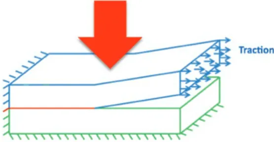
In the ATP manufacturing process the conformed parts deform because of the residual stresses that were installed in the part due to thermoelastic loads applied during the tape placement (laser heating, roller pressure and the tension applied on the incoming tape), as sketched in Fig. 8.

Figure 8. Sketch of the thermo-mechanical loading during the ATP 5. Evaluating the residual stresses generated by the ATP process

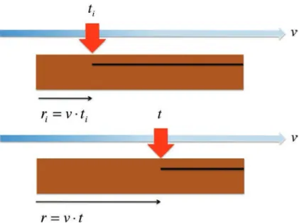
Even if the thermo-mechanical problem could be formulated in the laser-roller frame, as it was the case in the thermal model previously considered, in what follows we consider the frame related to the substrate that is assumed at rest. Thus, we can apply directly the PGD-based solver proposed in [10] and summarized in the previous section, but because of the time dependence on the temperature field in that frame we must solve the thermo-elastic problem at different instants that correspond to different positions of the couple laser-roller, as illustrated in Fig. 9.

Figure 9. Incremental thermo-mechanical coupling strategy

As previously described, the temperature field is accessible for any position of the thermal source. However, the mechanical model deserves more comments. First of all, it is important to notice that the geometry is changing with the interface welding after acting the laser-roller as illustrated in Fig. 10.

Figure 10. Evolution of the geometry during the interface welding

In Fig. 10 we can notice that the interface tip at time t is located at position r(t)= v !t .

We perform a sequence of PGD solutions of the thermo-elastic problem in the different geometries associated with different time instants uniformly distributed in the interval

t! 0,Lx

v

" #$

%

&', with a time step !t.

In order to compute the accumulated stresses at a certain cross-section, representative in first approximation of the ones installed at any location in the plate, we are computing

the stresses at the central section Lx

2 when the couple laser-roller moves from x= 0 to

x= Lx. When it reaches the right border x= Lx the stress state at the central

cross-section x= Lx

2 is frozen and it will be applied everywhere on the substrate when the

next tape will be placed, in order to determine the accumulated residual stresses induced

by the whole process that involve the placement of the Np plies composing the

laminate.

The thermo-elastic problem to be solved at time t during the placement of ply number

n is defined in the domain ! = 0, L

[

_x

]

" 0, L#$ _y%& " 0,L#$ _z%& where

Lz = n ! e = (n " 1)! e + e , being e the tape thickness and (n! 1)" e the substrate

thickness consisting of the n! 1 tapes already placed. An interface !(t) of length

possible discontinuity of the displacement field across it. The geometry and that interface are represented in figure 11.

Figure 11. Placement of tape number n

When placing the n ply, we perform at the first configuration (the one at t= 0 with the

thermal source located on the left border of the representative volume and the interface !(t = 0) crossing all the domain length because its tip is located at x = 0 ) the small transformations linear thermo-elastic calculation:

! "# = 0 # = C :

(

$%&" T M,t = 0

(

(

)

% T_ref

)

)

+#0(M) $ =!u + !u

( )

T 2 ' ( ) )) * ) ) ) (15)

where ! is the Cauchy’s stress tensor, ! the linearized deformation tensor, ! the

thermal expansion tensor, T_ref a reference temperature that in what follows will be

assumed to be the ambient temperature Tamb, C the fourth order elasticity tensor, u the

displacement field and !0(M) the accumulated residual stress field installed in the

substrate because of the previous tape placements. The temperature at each position

M!" and time t can be obtained as previously described from the steady state

temperature field obtained in the laser-roller frame.

As shown in Fig. 8 the substrate and the incoming tape are assumed clamped on its left border as well as in the bottom one in contact with the work-plane. In the remaining part of the domain boundary tractions are assumed known, being null everywhere except at the right border of the incoming tape, as Fig. 11 illustrates, where a traction F applies. Then, at the subsequents configurations, as the intermediate one depicted in Fig. 11, the stresses evolve because of the heating combined with the interface welding that prevents a stress-free cooling process. The stress evolution is calculated from the solution of

∇ ⋅ Δ

( )

σ = 0 Δσ = C : Δ

(

ε−α⋅ T M,t

(

( )

− T M,t − Δt

(

)

)

)

Δε= ∇ Δu

( )

+ ∇ Δu

(

( )

)

T 2 ⎧ ⎨ ⎪ ⎪⎪ ⎩ ⎪ ⎪ ⎪ (16)

where Δ •

( )

refers to the variation of the variable

( )

• between two consecutive time

steps: t− Δt and t.

In the previous thermo-mechanical problems (15-16), as it was also the case when the thermal model was addressed, the effects related to the changes of phase (solidification, crystallization …) are in first approximation neglected, as well as their associated inelastic behaviors (viscoelasticity, plasticity …).

The solution of those models was performed by applying a PGD strategy based on an in-plane-out-of-plane separated representation of the displacement field:

u x, y, z

(

)

= u x, y, z

(

)

v x, y, z

(

)

w x, y, z

(

)

⎛ ⎝ ⎜ ⎜ ⎜ ⎜ ⎞ ⎠ ⎟ ⎟ ⎟ ⎟ ≈ u_xyi

( )

_{x, y ⋅u} z i

( )

_z v_xyi

( )

_{x, y ⋅ v} z i

( )

_z w_xyi

( )

_{x, y ⋅ w} z i

( )

_z ⎛ ⎝ ⎜ ⎜ ⎜ ⎜ ⎞ ⎠ ⎟ ⎟ ⎟ ⎟ i=1 i= N

∑

(17)

Moreover, to ensure the eventual discontinuity of the displacement field across the

interface Γ(t) , we defined the functions χ x, y

( )

and ξ(z) , expressed by:

χ(x, y) = 0 if x≤ r(t) x− r(t) if x > r(t) ⎧ ⎨ ⎪ ⎩⎪ (18) and ξ(z) = 0 if z≤ (n − 1) ⋅ e 1 if z> (n − 1) ⋅ e ⎧ ⎨ ⎪ ⎩⎪ (19)

from which we can rewrite the separated representation (16) as:

u x, y, z

(

)

= u x, y, z

(

)

v x, y, z

(

)

w x, y, z

(

)

⎛ ⎝ ⎜ ⎜ ⎜ ⎜ ⎞ ⎠ ⎟ ⎟ ⎟ ⎟ ≈ χ(x, y)⋅ξ(z)⋅u1_xy x, y

( )

⋅u1_z z

( )

χ(x, y)⋅ξ(z)⋅ v1_xy

( )

_{x, y ⋅ v} z 1

( )

_z χ(x, y)⋅ξ(z)⋅ w1_xy

( )

_{x, y ⋅ w} z 1

( )

_z ⎛ ⎝ ⎜ ⎜ ⎜ ⎜ ⎞ ⎠ ⎟ ⎟ ⎟ ⎟ + + u_xyi

( )

_{x, y ⋅u} z i

( )

_z v_xyi

( )

_{x, y ⋅ v} z i

( )

_z w_xyi

( )

_{x, y ⋅ w} z i

( )

_z ⎛ ⎝ ⎜ ⎜ ⎜ ⎜ ⎞ ⎠ ⎟ ⎟ ⎟ ⎟ i=2 i= N

∑

(20)

that ensures the displacement discontinuity across the interface Γ(t) and the required continuity elsewhere. This kind of discontinuous enrichment constitutes the so-called dPGD, where “d” refers to its discontinuous character.

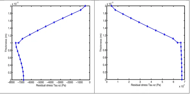
When applying this procedure (thermal calculation – discussed in section 3 - and the associated induced stresses just described) we can obtain the final stress distribution along a representative cross-section of a laminate, as shown in Fig. 12 that compares the

residual stresses σxxalong the laminate thickness for a laminate composed of two plies

(where for the sake of simplicity we considered the placement of the upper ply on a stress-free substrate composed of a single ply) both having the same reinforcement orientations (left figure) or being perpendicular orientations (right figure). Fig. 13 shows

similar results for the shear component of the residual stress σxz.

Figure 12. Residual stress σ_xx along the laminate thickness: (left) the reinforcement

orientation of both plies is the same; (right) both orientations are orthogonal

ï2 0 2 4 6 8 x 105 0 0.2 0.4 0.6 0.8 1 1.2 1.4 1.6 1.8 2x 10 ï3

Residual stress Sigmax xx (Pa)

Thickness (m) ï1 0 1 2 3 4 5 6 7 x 105 0 0.2 0.4 0.6 0.8 1 1.2 1.4 1.6 1.8 2x 10 ï3

Residual stress Sigmax xx (Pa)

Figure 13. Residual shear stress σxz along the laminate thickness: (left) the reinforcement orientation of both plies is the same; (right) both orientations are

orthogonal

As it can be noticed in Figs. 12 and 13 the first configuration, equal reinforcement orientations does not imply significant residual stresses so the distortion of the part will be inappreciable. However, in the case of an unbalanced laminate the residual stresses become more significant and a noticeable springback is obtained after demoulding as shown in Fig. 14.

Figure 14. Springback induced by the ATP residual stresses

ï8000 ï7000 ï6000 ï5000 ï4000 ï3000 ï2000 ï10000 0 0.2 0.4 0.6 0.8 1 1.2 1.4 1.6 1.8 2x 10 ï3

Residual stress Tau xz (Pa)

Thickness (m) 0 1 2 3 4 5 6 7 x 104 0 0.2 0.4 0.6 0.8 1 1.2 1.4 1.6 1.8 2x 10 ï3

Residual stress Tau xz (Pa)

6. Conclusions

The evaluation of residual stresses induced by the automated tape placement process requires three distinct steps. The temperature field in the laminate has to be first calculated. Several approaches are conceivable. Here, we solve the thermal problem in the coordinate system attached to the heating device. The line speed is therefore explicitly introduced in the formulation of the problem by adding a convection term. The Proper Generalized Decomposition proceeds by decoupling the space coordinates by performing an in-plane/out-of-plane decomposition that allows solving the 3D problem with the computational complexity characteristic of 2D solutions. Moreover, the fiber orientation of each ply can be introduced as an extra-coordinate of the model and a parametric solution valid for a large range of laminates (sequencing of plies) can then be computed. Other extra-coordinates can be also introduced allowing efficient material and process identification and/or optimization.

The mechanical problem is solved incrementally in a representative volume. The laser moves progressively along the placement direction. For a given position, a thermo-mechanical problem is solved, making use of the temperature field already computed. The residual stress is obtained by considering the evolution of the stress on the central cross-section of the representative volume.

Finally, with the residual stresses just obtained, the part can be demoulded and the induced distortion can be calculated by solving the associated elastic problem at the structure level again by invoking the in-plane-out-of-plane PGD decomposition of the associated elastic problem.

Nevertheless, very simple configurations were analyzed and this work has still to be validated with more complex simulations and experiments that constitute a work in progress.

References

1 Sonmez F.O., Hahn H.T., Akbulut M., Analysis of process-induced residual stresses in tape placement, Journal of Thermoplastic Composite Materials, 2002, 15, pp. 525-544.

2 Pitchumani R., Ranganathan S., Don R.C., Gillespie J.W., Analysis of transport phenomena governing interfacial bonding and void dynamics during thermoplastic tow-placement, International Journal for Heat Mass Transfer, 1996, 39, pp. 1883-1897.

3 Schledjewski R., Latrille M., Processing of unidirectional fiber reinforced tapes fundamentals on the way to a process simulation tool (ProSimFRT). Composites Science and

Technology, 2003, 63/14, pp. 2111-2118.

4 Lamontia M., Gruber M., Tierney J., Gillespie J., Jensen B., Cano B., Modeling the accudyne thermoplastic in situ ATP process. SAMPE Europe, March 2009, Paris.

5 Ammar A., Mokdad B., Chinesta F., Keunings R., A new family of solvers for some classes of multidimensional partial differential equations encountered in kinetic theory modeling of complex fluids. Journal of Non-Newtonian Fluid Mechanics, 2006, 139, pp.153-176.

6 Ammar A., Mokdad B., Chinesta F., Keunings R., A new family of solvers for some classes of multidimensional partial differential equations encountered in kinetic theory modeling of complex fluids. Part II: Transient simulation using space-time separated representation. Journal of Non-Newtonian Fluid Mechanics, 2007, 144, pp. 98-121.

7 Pruliere E., Chinesta F., Ammar A., On the deterministic solution of multidimensional parametric models by using the Proper Generalized Decomposition. Mathematics and Computers in Simulation, 2010, 81, pp. 791-810.

8 Ghnatios Ch., Chinesta F., Cueto E., Leygue A., Breitkopf P., Villon P., Methodological approach to efficient modeling and optimization of thermal processes taking place in a die: Application to pultrusion. Composites Part A, 2011, 42, pp. 1169-1178.

9 Ghnatios Ch., Masson F., Huerta A., Cueto E., Leygue A., Chinesta F., Proper Generalized Decomposition based dynamic data-driven control of thermal processes. Computer Methods in Applied Mechanics and Engineering, 2012, 213 pp. 29-41.

10 Bognet B., Leygue A., Chinesta F., Poitou A., Bordeu F., Advanced simulation of models defined in plate geometries: 3D solutions with 2D computational complexity. Computer Methods in Applied Mechanics and Engineering, 2012, 201, pp. 1-12.

11 Regnier G.; Nicodeau C., Verdu J., Chinesta F., Cinquin, J., Une approche multi-physique du soudage en continu des composites à matrice thermoplastique : vers une modélisation multi-échelle. 18ème CFM, Grénoble 2007, http://documents.irevues.inist.fr/handle/2042/15971