To link to this article : DOI 10.1007/s10494-013-9466-8
URL : http://dx.doi.org/10.1007/s10494-013-9466-8
This is an author-deposited version published in: http://oatao.univ-toulouse.fr/ Eprints ID: 9132
To cite this version:
Kourta, Azeddine and Michel, Brice and Gajan, Pierre and Strzelecki, Alain and Boisson, Henri-Claude Improved Unsteady RANS Models Applied to Jet Transverse to a Pipe Flow. (2013) Flow Turbulence and Combustion, vol. 90. ISSN 1386-6184
O
pen
A
rchive
T
oulouse
A
rchive
O
uverte (
OATAO
)
OATAO is an open access repository that collects the work of Toulouse researchers and makes it freely available over the web where possible.
Any correspondence concerning this service should be sent to the repository administrator: [email protected]
DOI 10.1007/s10494-013-9466-8
Improved Unsteady RANS Models Applied to Jet
Transverse to a Pipe Flow
A. Kourta · B. Michel · H. C. Boisson · P. Gajan · A. Strzelecki
Abstract An unsteady RANS model is developed in order to simulate the complex situations involving both free and bounded flows. This model tuned to catch coherent flow structures is developed both in the k-ε and k-l approaches. The full 3D geometry of a round jet exiting from a reservoir into a pipe has been computed. Periodic conditions are applied in order to compare with an experiments consisting of eight jets exiting in a cross pipe flow. Improvement has been obtained with this URANS turbulence model compared to RANS and good agreement compared with experiment has been obtained. Unsteady phenomena are reproduced by the model and provide more insight into the physical properties of the flow and of the transport of a passive scalar.
Keywords URANS model · Jets · Cross flow · Numerical simulation · Mixing
1 Introduction
Current demands to optimize combustion performance and reduce pollutant emis-sions require considerable research efforts from gas turbine industry. The basic ob-jectives in combustor design are to achieve easy ignition, high combustion efficiency and minimum pollutant emissions. In this context, numerical methods are very
A. Kourta (
B
)Laboratoire PRISME, Université d’Orléans,
8 rue Léonard de Vinci 45072 Orléans Cedex 2, France e-mail: [email protected]
B. Michel · P. Gajan · A. Strzelecki
ONERA-the French Aerospace Lab, 31055 Toulouse, France H. C. Boisson
IMFT, CNRS, Université de Toulouse, INPT, av. du Prof. Camille Soulas, 31400 Toulouse, France
attractive alternatives compared to the expensive experimental set-ups facilities required in these research areas. In the last decade, experimental and numerical studies have indicated that unsteady phenomena play an important role in fuel injection, combustion processes and flow mixing [1]. Contrary to the Reynolds Averaged Navier-Stokes (RANS) equations which are restricted to steady turbulent flows, Direct Numerical Simulation (DNS), Large Eddy Simulation (LES) or at least Unsteady RANS (URANS) simulations reproduce flow unsteadiness allowing a better prediction of combustion efficiency or instabilities.
Nevertheless, in order to develop such numerical tools, it is necessary to validate them on flow conditions reproducing unsteady phenomena observed in actual com-bustion chambers. This is the case in the so-called dilution zone where an array of “cold” jets flow transversally into a main hot bulk flow coming from the combustion region. In this paper, the basic case of a collection of jets flowing into a pipe section is selected as representative of the physics of such dilution zone.
A large number of works has been published on jets in cross flow since sixty years because they are observed in many situations such as chimney stacks or estuary mixing for instance. The generic work of Fric and Roshko [2] can be considered as a good reference as it describes precisely the vortex dynamics in the zone surrounding the injection. The jet in transverse flow was also simulated using LES by Yuan et al. and the vortex flow configuration obtained in [2] is also observed and described by these authors. But in the case of the combustion chamber case, it is necessary to take the confinement (by an internal transverse flow) into account. Strzelecki et al. [4] have provided experimental results on the mixing of eight jets exhausting in a pipe flow using LDA, PIV, PLIF and HWA. This test case was used by Priere et al. [5] for the validation of LES simulations.
The objective of this paper is to validate a turbulence model consisting of a specific URANS approach on this flow configuration. It was shown by Kourta [6, 7], that this approach is suitable for predicting unsteady flow with coherent structures. The principle was validated by a first attempt of this family of models in the case of a detached shear layer downstream of a backward facing step by Aubrun et al. [8], where they compared the unsteady model to phase averaged measurements. Indeed the behaviour of vortices due to Kelvin-Helmholtz instability was fully recovered and turbulence was shown to be mainly dependant on coherent structures. The model used here was proposed by Kourta [6,7] and uses a non linear k-ε formulation. This formulation is compared with an alternative k-l model proposed by Michel [9] where l profiles having a linear like behaviour near walls could have some advantages.
Similar to this URANS approach, Time-dependent Reynolds Averaged Navier Stokes (T-RANS) approach [10,11] has been used to analyse the body force effects on the reorganisation of large coherent structures.
The models used are presented in the following section and the flow configuration tested in Section 3. Results for different unsteady RANS models are discussed in Section4.
2 Steady and Unsteady RANS Models
The starting point of the modelling approach is the decomposition of any instan-taneous physical variable into two parts. For the Reynolds averaging the decom-position consists on time averaging and fluctuating part. The unsteady approach
is based on the decomposition into coherent part and incoherent random part. In this case the coherent part is obtained by performing an ensemble averaging. This decomposition can be obtained by phase averaging that can capture the organized and coherent structures. The random part is represented by suitable model. It has been demonstrated that this decomposition is fully satisfied if pseudo-periodic com-ponents exist in the flow. It’s the case for the flow around circular cylinder where the Von Karman street contains this kind of structures and presents a single frequency. It’s more difficult to determine the situation for multi frequency phenomena. In this case, a special filtering operation, such as the one used by Brereton and Kodal [12] has to be performed. There is no restriction in deriving the suitable mathematical model, apart for the description of adequate and initial conditions for each phase-averaged variable of the flow. For both cases (steady or unsteady approach) the following relation can be written:
8 (xk,t)= 8 (xk)+ 8r(xk,t) or 8 (xk,t) = b8 (xk,t)+ φr(xk,t)
where 8 (xk)the time averaged part, 8r(xk,t)the corresponding random part with
8r(xk,t)= 0, b8 (xk,t) the coherent part and φr(xk,t) the corresponding random
part.
A condition to formally obtain adequate equations for the coherent part is to impose a zero cross-correlation:
µ ˆ8, φr
¶ = 0
between coherent and incoherent motions. In this case only quadratic interactions will appear for the random part of the fluctuation. The so called Leonard stresses do not exist in flow equations, not like in the LES approach. The resulting phase averaged Navier Stokes equations look identical to the Reynolds averaged Navier Stokes equations. Only the Reynolds shear stress is replaced by the phase averaged shear stress. In this study no filtering is used to establish the equations. In fact, for the numerical study, the efficiency of the decomposition is related to the turbulent model used. Such decomposition between coherent and incoherent part provides a set of partial differential equations that holds for all possible decompositions. The specific problem corresponding to a given practical filtering is then defined through adequate boundary conditions and modelling for unknown correlations.
Equations obtained in both cases have the same form the only difference is in the problem resolved by using one or other averaging and the closure model used. In the case where the mean flow is steady the Reynolds averaged equations are solved. The time τ serves as iterative time and does not have any physical signification. τ accounts only for reaching steady state. When τ is higher enough the steady solution is obtained.
In the presence of unsteady mean flow, the unsteady Reynolds averaged equations are solved. Also, because the solver uses the compressible equations the mass weighted averaging (Favre averaging) is performed in both cases.
e 8= ρ8 ¯ρ or e8= c ρ8 b ρ
The continuity equation is given in each case by: ∂ρ ∂τ + ∂ρ eUi ∂xi = 0 or ∂bρ ∂t + ∂bρ eUi ∂xi = 0
The momentum equations can be writing as follow: ∂¯ρ ˜Ui ∂τ + ∂ρ ˜UiU˜j ∂xj = − ∂P ∂xi + ∂ ∂xj ¡ ¯τij− ρuiuj ¢ ∂ρ ebUi ∂t + ∂ρ ebUiUej ∂xj = − ∂ bP ∂xi + ∂ ∂xj ¡ bτij− ρbuiuj ¢
And for the energy equation we have: ∂ρ eE ∂τ + ∂ρ eE eUi ∂xi = − ∂ ∂xi " P eUi+ ¡ ρuiuj− τij¢ eUj− (λ + λt) ∂T ∂xi # ∂bρ eE ∂t + ∂ρ ebE eUi ∂xi = − ∂ ∂xi " b P eUi+ ¡ ρbuiuj− bτij¢ eUj− (λ + λt) ∂ bT ∂xi #
Unsteady Reynolds averaged Navier-Stokes equations with a k-ε or k-l models are solved. Models modified to be used in unsteady separated flows are compared to standards models. Standard models will be presented first and then the improved models.
2.1 Standard models
The standard models used are based on the turbulent viscosity concept. In this case the turbulent stresses are related to the deformation of the mean flow by a linear law as follow: −ρuiuj= 2µt µ eSij− 1 3eSkkδij ¶ − 2 3ρekδij
The turbulent viscosity µt is related to turbulent kinetic energy k and its dissipation
ε. For the k–l model the dissipation is replaced by the turbulent integral length scale
l. In both cases it’s given by:
µt= fµCµρ ek2 eε = fµC 1/4 µ ρek 1/2l
Where Cµ is a non-dimensional constant (Cµ = 0.09). The low Reynolds number approach is used here and then the transport equations for the turbulent quantities k and ε [9,13,14] are given by:
∂ρek ∂τ + ∂ρek eUj ∂xj = ∂ ∂xj "µ µ+ µt σk ¶ ∂ek ∂xj # − ρuiuj ∂ eUi ∂xj − ρεs ∂ρε ∂τ + ∂ρε eUj ∂xj = ∂ ∂xj ·µ µ+ µt σε ¶ ∂ε ∂xj ¸ − eε k " Cε1ρuiuj ∂ eUi ∂xj + f 2Cε2ρ (ε− εlam) # Where: εlam = 2ν k y2 w
,yw is the distance from the wall,
fµ = tanh2 µ 0.6+ Ret 12 ¶ , f2 = 1 − 0.3 exp " − µ Ret Cµ ¶2# and Ret= µt ± µ. With: σk = 1, σk = 1.3, Cε1 = 1.44 and Cε2 = 1.92
For the k–l model, the equation of l [9,13–15] used is: ∂ ¯ρl ∂τ + ∂ ¯ρl ˜Uj ∂xj = ∂ ∂xj ·µ µ+ µt σε ¶ ∂l ∂xj ¸ +µt lσl " A l ρC3/4µ k3/2 ρu′′iu′′j∂ ˜Ui ∂xj+B+C µ ∂l ∂xj ¶2 +Dl 2 k2 µ ∂k ∂xj ¶2 +El k ∂l ∂xj ∂k ∂xj # +βµ l à κ2 − µ ∂l ∂xj ¶2!
The damping constants and functions are as follow:
A B C D E β κ σl 0.02 0.14 −1 − fβ −34 fµ2 − 1 2 fβ+ 3 f 2 µ 0.4 0.435 1.3 fµ = tanh ³ Ret 21.3 ´ and fβ = 1 + Ret fµ d fµ dRet = 1 + 1− f2 µ fµ Ret 21.3 varying from 1 to 2.
2.2 Improved URANS approach
In this kind of flows, DNS (Direct Numerical Simulation) or at least LES (Large Eddy Simulation) are proper approaches to take account of small scales within a 3D framework. However, they require an enormous amount of resources for even simple geometry. An hybrid RANS/LES approach based on blending the best features of RANS and LES can be also used. Ideally, one could adequately simulate this class of flows with adapted unsteady RANS (URANS) technique [6–8]. However, the RANS turbulence models using linear turbulent viscosity models are well known to be dissipative and without caution unsteadiness can be damped. Here, the URANS model used is adapted to allow the unsteadiness development.
The starting point of the present approach is the decomposition of any instanta-neous physical variable into a coherent, organized part and an incoherent, chaotic part. Equations for the coherent part are obtained by performing an ensemble average of the instantaneous flow equations. The effects of the turbulent chaotic part are introduced by using a suitable unsteady turbulence model.
The closure law of turbulent stresses that was used is similar to the one obtained by Zhu and Shih [16], or Shih et al. [17] for steady flows. Assuming that the unknown correlations, resulting from the use of ensemble averaging, depend on the averaged velocity gradients, turbulent length, and velocity scales, a closure relation is derived by using the invariance theory. Using the realizability conditions [6, 14], the coefficients are found to be functions of both the strain rate and the rotation rate divided by the time-scale of the turbulence. Using the turbulent kinetic energy k and dissipation ε (for the k-ε model) to characterise the turbulent length and velocity scales, the averaged turbulent correlations can be derived.
An improved URANS model is based on the turbulent viscosity concept (for more details see [6,7]). Turbulent shear stress tensor is obtained by following Boussinesq relation: τij= −ρbuiuj= 2µt µ Sij− 1 3Skkδij ¶ − 2 3ρkδij
The turbulent viscosity is given by:
µt= Cµ·ρ
k2
ε
Cµ, the turbulent viscosity coefficient is related to deformation rate η and rotation rate ξ : Cµ(η, ζ )= 2 3 × 1 A1+ η + γ1ξ with η = k εS ξ = k εÄ
Where S is the deformation rate and Ä is the rotation rate. A1 is equal to 1.25 and
γ1 to 0.9. The calibration of model constants has been done by choosing appropriate
simple experiments, i.e. backward facing step shear layer [18] and planar jet [19]. In these experiments phase averaging has been used.
To close the equations, the averaged turbulent kinetic energy and its averaged dissipation are determined from the solution of their transport equations.
For the near wall region, the low turbulent Reynolds numbers treatment is used. The same damping function as the one used for the standard case is used.
The same procedure can be derived for the k-l model [9]. For the standard model instead of ε equation the equation of l is used:
l= C3/4
µ
k3/2
ε µt = ρCµ1/4k1/2l
Cµ has the same expression as the k-ε improved URANS model with:
η= l C3/4µ √ kS and ξ = l C3/4µ √ kÄ,S= q 2SijSij and Ä = p 2ÄijÄij
A careful reading of the above equations leads to the fact that coefficients η and ξ are acting as turbulent viscosity reducers in areas of high deformation and rotation rates. RANS equations can be solved with a time term acting as a relaxation term, and thus RANS modeling provides time independent solution only because the turbulent viscosity induces a very high diffusivity. It turn out that the proposed model is tuned towards a MILES [20] type model in the areas of high deformation and rotation rates, and consequently coherent structures can be captured. On the opposite, in areas of low deformation and rotation rates, the proposed model is tuned towards a RANS model and the turbulence is not solved but modeled.
The two models were implemented in the ONERA code dedicated for the simulation of compressible reactive flows. It contains different solvers each of them taking into account a physical aspect (turbulence, combustion, two phase dispersed flow, heat transfer...). This code uses unstructured grids and different integration schemes and permits calculation on parallel computers. Various boundary conditions are available. For the inlet and the outlet boundaries the subsonic non-reflecting conditions are used. At the wall, the adiabatic condition is prescribed and the velocity is equal to zero. When needed the symmetry condition can be applied.
3 The Test Flow Configuration
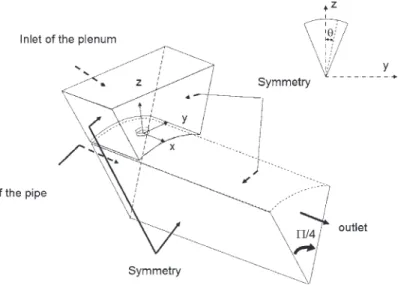
The flow configuration selected for testing the performance of the models is the in-jection through 8 circular holes (d = 6.1 mm) in a straight circular tube (D = 100 mm). The symmetry of the problem allows a reduced domain in the angular sector of π /4 (Fig.1). The inlet flow is established fully turbulent (turbulent intensity is imposed) and the outlet is free (external condition is imposed). The flow configuration is fully documented in Strzelecki et al. [4]. The injection is done inside a tranquilisation zone (plenum).
The mesh is a multi block structured coincident mesh of 380,000 volumes. It is refined near the walls and the orifice outlet and stretched to reach a uniform distribution far from the injection (Fig. 2). The first point near the wall is situated inside the viscous sublayer. The model used corresponds to a low Reynolds number model at the wall. The mesh dependences have been studied. More refined mesh was
Fig. 1 The test flow
Fig. 2 Detail of the refined
mesh adopted
tested. The solution predicted with the refine mesh is the same as the one obtained with the mesh used in this study [9]. This means that the solution presented here is not mesh dependent. The important goal here is to use the same mesh to test and to compare steady and unsteady Reynolds averaging turbulence models.
Longitudinal velocity and turbulent kinetic energy profiles issued from the LDA measurements are imposed at the inlet of the pipe. It corresponds to a bulk velocity U0 equals to 25 m/s and turbulent intensity at the centre of the pipe of 5 %. For the
plenum, a uniform condition is imposed at its inlet. Its value is chosen to obtain the jet velocity (Ujet)of 80 m/s (Ujet = 3.2U0). Considering the ratio between the hole
and the plenum surfaces:
Rs= Shole Sb ox = 29× 10−6 1609× 10−6 = 18.10 −3
it can be obtained that: UBC_b ox = Rs× Ujet = 1.44m
±
s
Hence the mass flow injected is Qjet = 2.88 × 10⁻³kg/s and the mass flow of the
mean field is Q0 = 29.13 × 10⁻³kg/s. So the mass flow ratio is approximately 0.1.
The turbulence level is fixed to 15 % of the mean velocity (0.05 m2/s2). A reference
integral length is fixed to 1 mm (or ε = 1.84 m2/s3)to represent the turbulence length
scale imposed in the experiment by the grid generating a turbulence in the plenum.
4 Results
4.1 Computational parameters effect
The effect of time integration is studied both on RANS and URANS computations to select the optimal method. For RANS models two time schemes have been tested. An implicit first order scheme using gradient reduction method of GMRES type
and second order Runge-Kutta implicit scheme were used. The velocity profile and turbulent kinetic energy are approximately identical for both schemes [9].
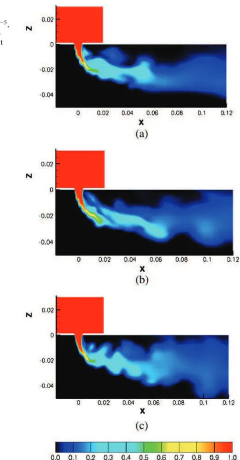
For the URANS model, the time step effect was studied. 1t equals to 5.10−5 and 10−5 s were tested. The quality of the results is better with the smaller time step. The
Fig. 3 Instantaneous
concentration of passive scalar: (a): implicit 1t = 10−5, 1st order, (b): implicit 1t = 10−5, 2nd order, (c): explicit 1t = 10−7, 2nd order
computations were done both with implicit and explicit second order Runge-Kutta scheme. With second order scheme a better description of the flow is obtained. Small coherent vortices were captured in the wake. The implicit scheme can introduce numerical diffusion. The precision is generally better with explicit scheme. This scheme allows a more precise numerical resolution (Fig.3), less numerical dissipation and better agreement with experimental results. Explicit scheme has to respect the CFL condition. The time step is very small and so to have enough flow evolution to do complete analysis huge computational time is needed. However, when needed, it’s possible to obtain approximately the same precise results with very much lower computational time.
Explicit scheme needs longer time to obtain enough information to perform suitable analysis. With less numerical iteration, implicit 2nd order scheme leads approximately to the same results. Computations were done with this last scheme.
4.2 Mean flow
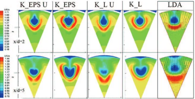
Four different models are compared with LDA measurements results in Fig. 4. Here the longitudinal velocity is made non-dimensional by the cross-flow mean bulk velocity U0. The steady classical RANS models are called standard (std) and they
are compared with URANS models (U). Both models are applied in very similar conditions and with the same near wall function to account for the low Reynolds number effects. The grid and the numerical schemes are the same in the four cases. The overall mean structure of the flow is more or less correctly represented by all these computations. In the neighbourhood of the jet (x/d = 2), the models predict main jet zones larger than the ones measured in the experiments but all model results are similar. Further downstream at x/D = 5 only the URANS models provide results that are close to the experiments. Thus the standard models turn to be too diffusive and only the unsteady ones represent the physics of the cross jet.
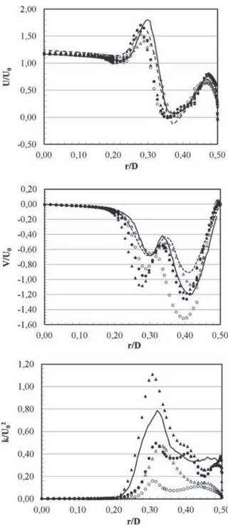
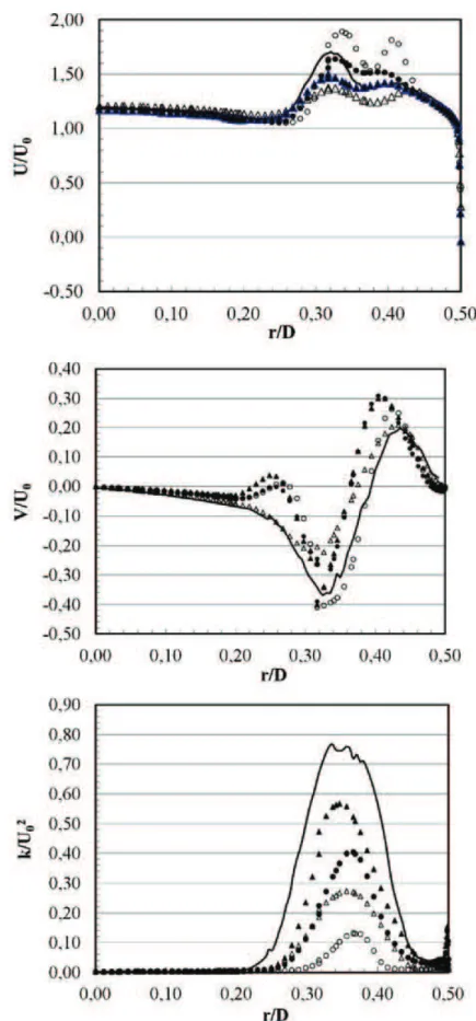
To confirm this qualitative result, the velocity and turbulent kinetic energy profiles computed at x/d = 2 along the radial direction are compared in Figs. 5 and 6 for two angular orientations (θ qual to 0 and π /16 respectively). The components of the velocity are non-dimensionalized by the cross-flow mean bulk velocity U0 and
the turbulent kinetic energy by U2
0. The ordinate r follows the duct radius (0 at
the center-line and maximum at the duct wall) and is scaled by D the main-pipe diameter.
Similar behaviours of the curves are obtained for the mean velocity components (U and V) for numerical and experimental results. Nevertheless, on the RANS and URANS curves for the U component, a shift toward the pipe axis of the maximum velocity is observed compared to the LDA measurements. This corresponds to an over penetration of the jets in the pipe flow. The better results obtained with the
Fig. 5 Mean velocity
components and turbulent kinetic energy profiles (x/d = 2; θ = 0; 2nd order scheme) (continuous line: LDA measurements; dashed line: LES, △: k-l; °: k-ε; N: k-l URANS, : k-ε URANS)
Fig. 6 Mean velocity
components and turbulent kinetic energy profiles (x/d = 2; θ = π/16; 2nd order scheme) (continuous line: LDA measurements; △: k-l; °: k-ε; N: k-l URANS, : k-ε URANS)
URANS methods underline the necessity to take into account the non isotropic effect of large scale structures on the flow mixing. As a confirmation of this necessity, a better accordance was even observed with the LES method developed by Priere et al. [5] on the same configuration but with considerably higher computational resources.
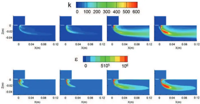
Fig. 7 Turbulent kinetic energy and dissipation evolution for different turbulent models
For the other components and for kinetic energy the unsteady models provide better results than the steady ones.
The turbulent kinetic energy (TKE) obtained with the unsteady models and plotted in Figs. 5 to 7 is the sum of coherent (unsteady organized) and random (turbulent) averaged TKE. Therefore, in areas where turbulence is dominated by strongly coherent structures, for instance in the shear layer of the jets, the random (modelled) TKE is reduced compared to RANS model, but the sum is sensibly higher (Figs. 5 to 7). Comparisons of TKE profiles with LDA measurements are greatly improved thanks to the unsteady computations. In the plane axis, the k-l over predicts the turbulent kinetic energy while the k-ε under predicts it. In the off axis plane the unsteady models are much closer to the measurements but both k-ε and k-l predict lower TKE. The conclusion is that the prediction of mean value of velocity and turbulence is improved by using the unsteady models even in this position for which the velocity maps seem to be quite similar for all the models.
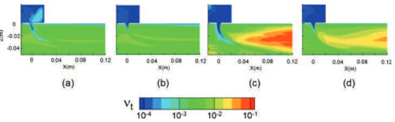
Fig. 9 Turbulent viscosity: k-ε (a), k-l (b), URANS: k-ε (c) and k-l (d)
The turbulent kinetic energy and dissipation contours are presented on Fig.7for different models. An increase of the kinetic energy corresponds to an increase of the dissipation. Significant differences can be observed between the standard models and URANS ones. These differences are related to the turbulent viscosity coefficient Cµ. This coefficient is constant and equals to 0.09 for the standard model and variable in the improved models. Cazalbou and Bradshaw [21] have been concluded that this coefficient is strongly dependent on the flow characteristics. They also indicate that Rodi [22] observed for this coefficient a range from 0.03 to 0.6 and is strongly depend on Reynolds number. An increase of the Reynolds numbers leads to a decrease of this coefficient. For higher Reynolds numbers, this coefficient has asymptotic lower value of approximately 0.05 for boundary layer and 0.065 for channel flow [21]. The values obtained with URANS models are between 0.005 and 0.4 in the shear layer and in the wake (Fig.8).
The turbulent viscosity νtdistributions are therefore very different for both classes of models (Fig. 9). For standard turbulence models, the observed behaviour is not adequate. Indeed, in the shear layer and in the wake region where the production supposed to be large, the turbulent viscosity is uniformly small. However, for the improved URANS model, the turbulent viscosity is small in the jet and initial shear layers. In this region, because the local effective viscosity is small, the coherent structures are dominant and develop from natural instabilities. In the wake where the turbulence is important the turbulent viscosity has high values.
The ultimate goal of this work is to consider the ability of the chosen models to predict passive scalar transfer and mixing. The actual URANS models improve this
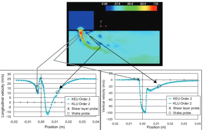
-120 -100 -80 -60 -40 -20 0 20 -0,02 -0,01 0,00 0,01 0,02 0,03 0,04 Position (m) V e rt ic a l v e lo c it y ( m /s ) -15 -10 -5 0 5 10 15 20 25 30 -0,02 -0,01 0,00 0,01 0,02 0,03 0,04 Position (m) L o n g it u d in a l v e lo c it y ( m /s ) KEU Order 2 KLU Order 2 Shear layer probe Wahe probe
KEU Order 2 KLU Order 2 Shear layer probe Wake probe
Fig. 11 Sensors positions in the instantaneous velocity field (top) and in the mean velocity profiles
(bottom)
prediction with respect to standard models. The concentration of a passive scalar has been computed in the present situation. It is introduced at the input section with a constant imposed value and transported by the flow in a domain limited by non permeable walls and a constant flux at the exit. The experiments of Strzelecki et al. [4] are designed to reproduce this situation. On Fig. 10 the URANS k-ε model prediction is compared to PLIF measurements of concentration field. The comparison is judged satisfying and representative of the physics of the mixing phenomenon.
4.3 Frequency and vortex shedding
In this section we are more concerned with the unsteadiness induced by vortex shedding mechanisms in the flow. These are mainly observed directly near the
Fig. 12 Signals at point A (left) and point B (right) (continuous line: k-l URANS, dashed line: k-ε
Fig. 13 Spectra of longitudinal velocity fluctuation on point A
injection (Point A) and further in the wake of the wake region (Point B). At these two points, sensors are used both in experiment and computation to better analyse the unsteadiness properties of the flow. On Fig.11these two points are selected on a line parallel to the wall of the pipe. The results for the mean longitudinal and normal velocity profiles on this line are identical for both selected models.
For point A (Fig.12), the results show that the URANS modelling is the important key to predict unsteadiness in turbulent unsteady flows. Both unsteady RANS
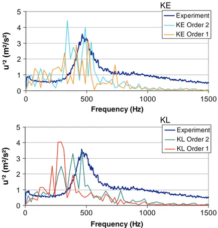
Fig. 14 Frequency distributions in the wake (point B) KE KL 0 1 2 3 4 5 0 500 1000 1500 Frequency (Hz) u '² ( m ²/ s ²) Experiment KE Order 2 KE Order 1 0 1 2 3 4 5 0 500 1000 1500 Frequency (Hz) u '² ( m ²/ s ²) Experiment KL Order 2 KL Order 1
Fig. 15 Frequency
distribution in the wake with URANS models: k-ε and k-l
0 1 2 3 4 5 0 500 1000 1500 Frequency (Hz) u '² ( m ² /s ² ) Experiment KE Order 2 KL Order 2
models predict a vortex shedding mechanism at the exit comparable to the one found in the experiments. The signal is perfectly periodic near the exit (point A) but quasi-periodic in the wake (B).
The FFT provides the power spectra density distribution (Fig.13). The temporal scheme has an important effect on the frequency obtained. Depending on the accuracy of the time step used, the frequency of vortex shedding can be different. This shows the importance for this kind of flow to use second order time accurate scheme. The value of the peak frequency obtained with the k-ε model is closer to the experiment. So this model can be considered as more reliable.
In the wake, the motion is related to the large scale and it is captured indepen-dently on the temporal scheme used as can be observed on Fig. 14. The dominant frequency is close to 500 Hz which is the same as the one obtained experimentally with hot wire anemometry. The improved URANS model is well adapted to predict this flow.
Both improved URANS k-ε and k-l models predict the unsteady behaviours of the flow when the 2nd order temporal scheme (Fig.15).
5 Conclusion
URANS turbulence model developed to predict turbulence flows in presence of coherent structures has been applied successfully to characterise the jet transverse to a pipe flow. Different numerical parameters have been evaluated to select adapted numerical scheme. The explicit and implicit schemes have been tested. If the explicit scheme is more precise and less dissipative, it’s need large computational time. The implicit scheme even if it’s more dissipative, can provide approximately the same results if the time step is adapted to the computations. In this work the implicit scheme is then chosen to compare different two equations eddy turbulent viscosity models. So, the flow has then been computed with standard RANS turbulence model and improved URANS one for k-ε and k-l approaches. Both main and unsteady characteristics have been compared to experimental data. Concerning the mean flow, in the neighbourhood of the jet, all models predict the main jet zones larger than experiments. Further downstream, only URANS models provide results in good agreement with experiments. Standard models are too diffusive. The mean value of velocity and turbulence are improved by suing URANS model. The fact that the
viscosity coefficient Cµis flow dependent improves the obtained results. Concerning the unsteady mechanism and vortex shedding, when the adapted numerical scheme is used both URANS k-ε and k-l models predict the unsteady behaviours of the flow. The flow dominant frequency is captured and the large scale motion is predicted. So it can be concluded that our URANS models perform better than standard models. Good agreement with experiment was obtained not only for the main evolution but also for unsteadiness. Frequency distribution has been captured.
Acknowledgements This work takes part of the EGISTHE program (Études Générales Inno-vantes Sur les Turbines Hautement Économiques) funded by the French Government through the Délégation Générale pour l’Armement (DGA).
References
1. Poinsot, T., Veynante, D.: Theoretical and Numerical Combustion. R.T. Edwards (2005) 2. Fric, T.F., Roshko, A.: Vortical structure in the wake of a transverse jet. J. Fluid Mech. 279, 1–47
(1994)
3. Yuan, L., Street, R., Ferziger, J.H.: Large eddy simulation of a round jet in cross flow. J. Fluid Mech. 19, 31–70 (1993)
4. Strzelecki, A., Gajan, P., Gicquel, L. Michel, B.: Experimental investigation of the mixing of transverse jets in circular pipe: non-swirling flow case. AIAA J. 47(5), 1079–1089 (2009)
5. Priere, C., Gicquel, L., Gajan, P., Strzelecki, A., Poinsot, T., Berat, C.: Experimental and Numerical Studies of Dilution Systems for Low-Emission Combustors. AIAA J. 13(8), 1753– 1766 (2005)
6. Kourta, A.: Computation of vortex shedding in solid rocket motors using time-dependent turbu-lence model. J. Propulsion Power 15(3), 390–400 (1999)
7. Kourta, A.: Instability of channel flow with fluid injection and parietal vortex shedding. Comput. Fluids 33, 155–178 (2004)
8. Aubrun, S., Kao, P.L., Boisson, H.C.: Experimental coherent structures extraction and numerical semi-deterministic modelling in the turbulent flow behind a backward-facing step. Exp. Thermal Fluid Sci. 22, 93–101 (2000)
9. Michel, B.: Caractérisation aérodynamique d’un écoulement avec injection pariétale de type dilution giratoire en vue de sa modélisation. PhD thesis, University of Toulouse, France (2008)
10. Hanjalic, K., Kenjeres, S.: T-RANS simulation of deterministic eddy structure in flows driven by thermal buoyancy and Lorentz force. Flow Turbul. Combust. 66, 427–451 (2001)
11. Kenjeres, S., Hanjalic, K.: Tackling complex turbulent flows with transient RANS: a review. Fluid Dyn. Res. 41(1), Article Number: 012201 (2009)
12. Brereton, G., Kodal, A.: An adaptive turbulence filter for decomposition of organized turbulent flows. Phys. Fluids 6(5), 1775–1786 (1994)
13. Vuillot, F., Scherrer, D., Habiballah, M.: CFD code validation for space propulsion applica-tions. In: 5th International Symposium on Liquid Space Propulsion, Chattanooga, Tennessee (2003)
14. Chevalier, P., Courbet, B., Dutoya, D., Klotz, P., Ruiz, E., Troyes, J., Villedieu, P.: CEDRE: development and validation of a multiphysic computational software. 1st European Conference for Aerospace Sciences (EUCASS), Moscow, Russia (2005)
15. Smith, B.R.: The k-kl Turbulence Model and Wall Layer Model for Compressible Flows, AIAA Paper, pp. 90–1483 (1990)
16. Zhu, J., Shih, T.: Computation of confined coflow jets with three turbulence models. Int. J Numer Meth Fluids 19, 939–56 (1994)
17. Shih, T., Zhu, J., Lumeley, J.: A realizable Reynolds stress algebraic equation model. NASA Technical Memorandum 105993, ICOMP-92-27; CMOTT-92-14 (1993)
18. Aubrun, S.: Etude expérimentale des structures cohérentes dans un écoulement turbulent décollé et comparaison avec une couche de mélange. PhD thesis INPT Toulouse, France (1998)
19. Faghani, D.: Etude des structures tourbillonnaires de la zone tourbillonnaire d’un jet plan: approche stationnaire multidimensionnelles. PhD thesis INPT Toulouse, France (2000)
20. Nakamori, I., Ikohagi, T.: Dynamic of hybridization of MILES and RANS for predicting airfoil stall. Comput. Fluids 37, 161–169 (2008)
21. Cazalbou, J.B, Bradshaw, P.: Turbulent transport in wall-bounded flows: evaluation of model coefficients using direct numerical simulation. Phys. Fluids 12, 3233–3239 (1993)
22. Rodi, W.: The prediction of free turbulent boundary layers by the use of a two-equation model of turbulence. PhD thesis, University of London (1972)