Marées rouges et distribution des assemblages palynologiques le long de la côte Ouest mexicaine

MARÉES ROUGES ET DISTRIBUTION DES ASSEMBLAGES PALYNOLOGIQUES LE LONG DE LA CÔTE OUEST MEXICAINE

MÉMOIRE PRÉSENTÉ

COMME EXIGENCE PARTIELLE

DE LA MAÎTRISE EN SCIENCES DE LA TERRE

PAR

AUDREY LIMOGES

UNIVERSITÉ DU QUÉBEC À MONTRÉAL Service des bibliothèques

Avertissement

La diffusion de ce mémoire se fait dans le respect des droits de son auteur, qui a signé le formulaire Autorisation de reproduire et de diffuser un travail de recherche de cycles supérieurs (SDU-522 - Rév.01-2006). Cette autorisation stipule que «conformément

à

l'article 11 du Règlement no 8 des études de cycles supérieurs, [l'auteur] concède

à

l'Université du Québec

à

Montréal une licence non exclusive d'utilisation et de publication de la totalité ou d'une partie importante de [son] travail de recherche pour des fins pédagogiques et non commerciales. Plus précisément, [l'auteur] autorise l'Université du Québec

à

Montréal

à

reproduire, diffuser, prêter, distribuer ou vendre des copies de [son] travail de recherche

à

des fins non commerciales sur quelque support que ce soit, y compris l'Internet. Cette licence et cette autorisation n'entraînent pas une renonciation de [la] part [de l'auteur]

à

[ses] droits moraux ni

à

[ses] droits de propriété intellectuelle. Sauf entente contraire, [l'auteur] conserve la liberté de diffuser et de commercialiser ou non ce travail dont [il] possède un exemplaire.»

Je souhaite remercier très sincèrement Anne de Vernal pour la direction de ce projet de maîtrise, sa confiance, ses encouragements et le soutien financier nécessaire à la réalisation de ce travail.

Un grand merci également à Ana Carolina Rufz-Fernandez pour l'organisation de la campagne d'échantillonage BIO El Puma TEHUA V, l'excellent accueil à Mazatlan et son support à distance. Son énergie débordante est une source d'inspiration.

Je tiens spécialement à remercier Taoufik Radi pour son aide et sa participation inestimables tout au long de ce projet. Ses nombreux conseils, sa patience et sa disponibilité au cours des deux dernières années ont grandement contribué à mener à bien cette étude.

Merci à Maryse Henry pour son aide lors des analyses palynologiques.

Merci à mes collègues et amis du laboratoire GEOTOP et particulièrement à Linda Genovesi pour sa précieuse complicité au cours des 2 dernières années. Merci à Benoît Thibodeau pour ses conseils et les nombreux pots massons partagés. Merci à Christelle Not pour son amitié et toute son implication au sein de la vie étudiante. Finalement, un énorme merci à mes parents, mes sœurs et mes beaux-frères pour leur soutien continuel.

AVANT-PROPOS

Ce document présente l'étude Marées rouges et distribution des assemblages palynologiques le long de la côte Ouest mexicaine qui a été réalisée dans le cadre d'un projet de collaboration entre le Québec et le Mexique. Cette étude visait l'identification des paramètres environnementaux favorables aux marées rouges et les objectifs spécifiques du projet étaient:

• Développer une base de données de référence de la distribution géographique des kystes de dinoflagellés (dinokystes).

• Caractériser la relation existant entre les assemblages de dinokystes et les paramètres environnementaux du milieu.

Cette étude est présentée sous forme d'article à l'intérieur du chapitre J. Cet article a été soumis à la revue Marine Micropaleontology. L'ensemble des échantillonnages, traitements de laboratoire et analyses des sédiments provenant de la marge Ouest mexicaine, ainsi que la rédaction de ce document ont été réalisés par Audrey Limoges. La contribution de chacune des personnes figurant comme co-auteur est la suivante: les données palynologiques obtenues par Kielt (2006) ont été combinées à celles provenant de ce projet afin de développer une base de données de référence plus étendue pour les basses latitudes. Les observations taxonomiques effectuées par Radi Taoufik ont permis de perfectionner la section consacrée à la systématique des dinokystes rencontrés le long de la côte Ouest mexicaine. L'ensemble des opérations d'échantillonnage des sédiments analysés au cours de cette étude a été coordonné par Ana Carolina Ruiz-Fernandez au cours de la mission BIO El Puma TEHUA V. Finalement, ce projet a été dirigé par Anne de Vernal.

AVANT-PROPOS 1Il

LISTE DES FIGURES v

LISTE DES TABLEAUX... .. vii

LISTE DES APPENDICES viii

RÉslJMÉ... .IX

INTRODUCTION GENERALE... . 1

CHAPITRE 1

RED TillES AND DINOFLAGELLATE CYST DISTRIBUTION IN SURFACE SEDIMENTS ALONG TIffi WESTERN MEXlCAN COAST (14.76° N to 24.75° N)

Abstract.. .4

1. Introduction 5

2. Regional setting .. 10

2.1. Oceanographie circulation 10

2.2. lndustrial development along the coast 11

3. Materials and Methods 13

3.1. Sampling 13 3.2. Geochemical analyses 13 3.3. Palynological analyses 14 3.4. Statistical analyses 15 4. Resu1ts 21 4.1. Geochemical data 21 4.2. Palynomorph assemblages 21 4.3. Dinocyst assemblages 22 4.4. Statistical assemblages 23 5. Discussion 41

5.1. Sources qforganic matter .41

5.2. Distribution ofdinocyst assemblages in relationship with ocean conditions 42

6. Conclusions 44

CONCLUSION GÉNÉRALE 45

APPENDICES... .. .. 46

LISTE DES FIGURES

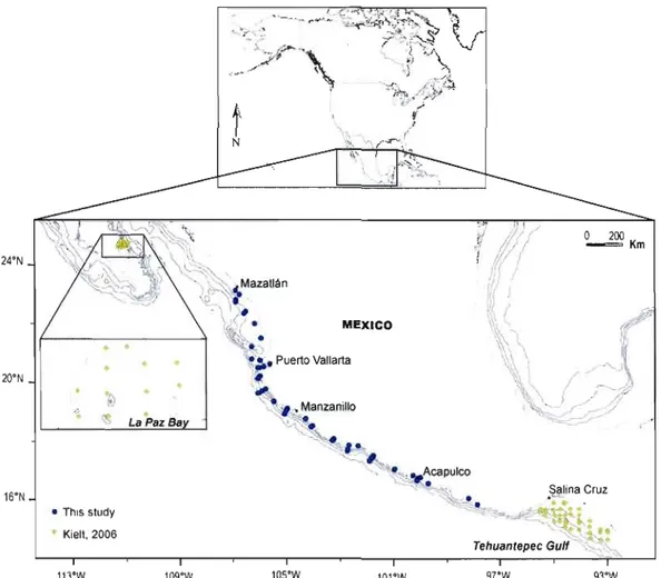
Figure 1. Carte de la zone d'étude et localisation des sites d'échantillonnage. Les points bleus correspondent aux sites d'échantillonnage de cette étude et les losanges verts correspondent aux sites d'échantillonnage de Kielt (2006). La bathymétrie est représentée par les isobathes 200, 500, 1000 et

2000 m 7

Figure 2. Circulation océanique de surface du Pacifique Nord Équatorial et vents dominants (flèches rouges) pour les périodes Hiver-Printemps et Été-Automne. CC: Courant de Californie; NEC: Courant Nord Équatorial; CCNE : Contre-Courant Nord Équatorial; CRC : Courant du Costa Rica; ITZC: Zone de convergence intertropicale (tiré de Kessler, 2006). Les points et les losanges

correspondent aux sites inclus dans la base de données 12

Figure 3. Résultats des analyses géochimiques effectuées sur les sédiments provenant de la marge Ouest mexicaine. (A) Rapports C:N et oUC des échantillons en fonction de la latitude; (B) Pourcentages en carbone organique et ol3C des échantillons en fonction de la distance par rapport à la

l3_C

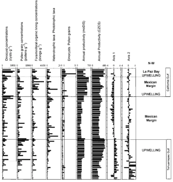
côte (km); (C) Pourcentages en carbone organique et o des échantillons en fonction de la profondeur (m); (D) Ol3C en fonction des rapports C :N des échantillons. Ces données ne sont pas disponibles pour les échantillons provenant de la Baie de La Paz et du Golfe de Tehuantepec 25 Figure 4. Résultats des analyses palynologiques pour les échantillons provenant de la marge Ouest mexicaine, de la Baie de La Paz et du Golfe de Tehuantepec (Kiel t, 2006): concentrations de dinokystes (kystes'g-I), concentrations de pollens (grains'g-I), concentrations de réseaux organiques de

foraminifères benthiques (réseaux organiques'g-I), rapport des espèces hétérotrophes sur les espèces

phototrophes de dinokystes, rapport des dinokystes sur les grains de pollens, productivité primaire estimée par le programme moDlS, productivité primaire estimée par le programme CZCS et axes 1et

2 provenant de l'analyse de redondance 26

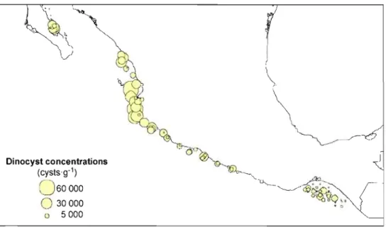
Figure 5. Distribution des concentrations totales de dinokystes (kystes'g-I) dans la zone d'étude ...28

Figure 6. Diagramme des pourcentages des principaux taxons de dinokystes. La pondération des spectres par rapport aux 2 premiers axes de l'analyse de redondance est illustrée à droite 31

Figure 7. Pourcentages des espèces hétérotrophes et phototrophes des assemblages de dinokystes ....32

Figure 8. Distribution des kystes de (A) Polysphaeridium zoharyi et (B) Lingulodinium machaerophorum dans la zone d'étude. La bathymétrie est représentée par les isobathes 200, 500,

1000 et 2000 m 33

Figure 9. Corrélation entre les pourcentages de taxons hétérotrophes dans les assemblages de dinokystes et la pondération des sites d'échantillonnage par rapport à l'axe 2 issu de l'analyse de redondance. L'axe 2 représente 29.4% de la variance et est corrélé significativement avec la

productivité primaire 37

Figure 10. Pondération des taxons et des paramètres environnementaux par rapport aux axes 1 et 2 issus de l'analyse de redondance. La liste des abréviations des taxons se retrouve au tableau 2 ...38

Figure 11. Distribution des assemblages de dinokystes par rapport aux axes 1 et 2 issus de l'analyse de

redondance 39

Figure 12. Pondération des sites d'échantillonnage par rapport aux axes 1 et 2 issus de l'analyse de redondance.

LISTE DES TABLEAUX

Tableau 1. Localisation des sites d'échantillonnage de la marge Ouest mexicaine 8

Tableau 2. Localisation des sites d'échantillonnage de la Baie de La Paz et du Golfe de Tehuantepec (Kiell,

2006) 9

Tableau 3. Liste des taxons de dinokystes recensés dans les sédiments, abréviations et regroupements de certaines

espèces pour l'analyse de redondance. . . . .. . .. .. . 17

Tableau 4. Paramètres environnementaux inclus dans J'analyse de redondance correspondant aux sites

d'échantillonnage: température des eaux de surface en été et en hiver (S_SST et W_SST), salinité des eaux de surface en été et en hiver (S_SSS et W_SSS), productivité des eaux de surface pour la période estivale, la période hivernale et l'année estimés par les programmes satellitaires moDIS et CZCS, profondeur (m) et distance par

rapport à la côte des sites d'échantillonnage 18

Tableau 5. Résultats des analyses géochimiques élémentaires et isotopiques des échantillons provenant de la

marge Ouest mexicaine... . 27

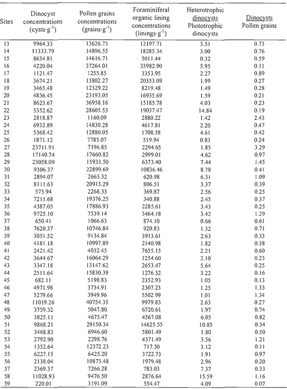
Tableau 6. Concentrations des palynomorphes terrestres (grains de pollens) et marins (dinokystes, réseaux

organiques de foraminifères benthiques), rapport des espèces hétérotrophes sur les espèces phototrophes de dinokystes et rapport des dinokystes sur les grains de pollens pour les échantillons de la marge Ouest

mexicaine 29

Tableau 7. Concentrations des palynomorphes terrestres (grains de pollens) et marins (dinokystes, réseaux

organiques de foraminifères benthiques), rapport des espèces hétérotrophes sur les espèces phototrophes de dinokystes et rapport des dinokystes sur les grains de pollens pour les échantillons de la Baie de La Paz et du

Golfe de Tehuantepec... . 30

Tableau 8. Pondération des taxons de dinokystes par rapport aux axes 1 et 2 issus de l'analyse de redondance ... 34

Tableau 9. Pondération des paramètres environnementaux par rapport aux 3 premiers axes issus de l'analyse de

redondance 35

APPENDICE A

Tableau de dénombrement d'es palynomorphes..,,, .. " .. " .. " "" "."." .. " .. " " ". " ". ".51

APPENDICE B Planche photographique 1 " " "."" " " " " " 55 Planche photographique 2 " " " , 57 Planche photographique 3 59 Planche photographique 4 "." " " " "." 61 APPENDICE C Systématique " "" "." '''''" " .. " " ".". " " , .. , 65

RÉSUMÉ

L'analyse palynologique de 47 échantillons de sédiment de surface provenant de la marge mexicaine (15 0

95 N à 23 0 11 N) a été réalisée afin de caractériser la relation existant

entre les kystes de dinoflagellés (dinokystes) et les paramètres environnementaux du milieu (température, salinité, productivité primaire, distance par rapport à la côte). Les observations permettent de diviser la zone d'étude en 4 régions caractérisées par des contextes hydrographiques distincts: la baie de La Paz, la marge Ouest mexicaine, le Nord du Golfe de Tehuantepec et le Sud du Golfe de Tehuantepec. Les taxons hétérotrophes dominent l'ensemble de ces assemblages à l'exception de ceux provenant du Sud du Golfe de Tehuantepec. Les concentrations totales de dinokystes suivent un gradient latitudinal décroissant avec des valeurs maximales dans la partie Nord de la zone d'étude.

Les traitements statistiques ont permis de démontrer que la distance par rapport à la côte, ainsi que les valeurs de productivité primaire sont les principaux paramètres déterminant la distribution des kystes de dinoflagellés. Les zones d'upwelling des baies de La Paz et de Tehuantepec présentent plusieurs similarités et leurs assemblages sont dominés par des taxons hétérotrophes tels Brigantedinium spp., Echinidinium spp, Polykrikos kofoidii et Selenopemphix quanta. Certaines espèces de dinokystes qui peuvent être à l'origine de marées rouges ont été observées à plusieurs sites. Lingulodinium machaerophorum est présent sur la marge Ouest mexicaine et dans le Nord du Golfe de Tehuantepec, alors que les concentrations de Polysphaeridium zoharyi sont plus fortes dans la zone d'upwelling du Golfe de Tehuantepec. La distribution des espèces liées aux marées rouges semble être influencée par le niveau de productivité primaire, ainsi que par la richesse en nutriments des eaux de surface.

Mots clés: Mexique, Dinokystes, Marées rouges, Paramètres environnementaux, Productivité pnmalre.

Le rrùlieu marin de la marge Ouest mexicaine est affecté par de fréquents épisodes de marées rouges. Les organismes planctoniques profitent du grand apport en éléments nutritifs résultant des activités humaines et des processus d'upwelling qui sont particulièrement intenses dans les régions du Golfe de la Californie et du Golfe de Tehuantepec (Mee et al., 1984; Alonso-Rodriguez and Ochoa, 2004). Ce domaine côtier présente une grande diversité de dinoflagellés parmi lesquels certaines espèces produisent des toxines très nocives pour les écosystèmes marins. Le transfert de ces toxines vers les niveaux trophiques supérieurs peut entraîner la mortalité massive des poissons. En plus des conséquences sur les écosystèmes marins, ce phénomène constitue une menace pour les industries de la pêche et du tourisme nationales.

Les dinoflagellés forment un groupe d'organismes planctoniques manns majeur composé d'espèces phototrophes, hétérotrophes et rrùxotrophes (e.g. Taylor and Pollingher, 1987; Gaines and Elbrachter, 1987). La présence des différentes espèces dans les rrùlieux marins est déterminée par leurs modes de nutrition respectifs: la disponibilité en nutriments et la pénétration de la lurrùère dans la colonne d'eau sont des caractéristiques du milieu vitales à la croissance des espèces phototrophes, alors que les espèces hétérotrophes dépendent principalement de la présence des diatomées et d'autres micro-organismes qui constituent leurs proies (Jacobson and Anderson, 1986). Au cours de leur période de reproduction, 10 à 20% des dinoflagellés produisent un kyste qui consiste en une enveloppe qui protège leur cellule pour une période de durée variable (Dale, 1976; Taylor and Pollingher, 1987; Head, 1996). Contrairement aux rrùcrofossiles carbonatés ou siliceux qui sont très sensibles aux processus de dissolution, les kystes de dinoflagellés (dinokystes) sont composés de matière organique très résistante permettant leur bonne préservation dans les sédiments. Ainsi, suite à des traitements physiques et chirrùques effectués sur les sédiments, les dinokystes peuvent être facilement isolés.

2 En milieu côtier, les assemblages de dinokystes dans les sédiments sont fortement liés aux conditions biotiques et abiotiques de la colonne d'eau. Leur distribution dépend des conditions des eaux de surface telles que la salinité, la température, la durée du couvert de glace et la productivité primaire (de Vernal et al. 1997, 200 1, 2005; Rochon et al., 1999; Radi and de Vernal, 2008). Les assemblages de dinokystes ont également été utilisés comme traceurs de la pollution anthropique (urbanisation, industrialisation) et du phénomène d'eutrophisation (Dale and Fjellsa, 1994; Dale, 1996).

Étant donné que les dinokystes se sont avérés être des traceurs efficaces 'pour la réalisation de reconstructions paléocéanographiques et paléoenvironnementales, plusieurs études ont été réalisées pour documenter leur distribution ((Dale and Fjellsa, 1994; Marret, 1994; Devillers and de Vernal, 2000; Radi and de Vernal, 2004; Radi et al., 2007; Pospelova et al., 2008; Zonneveld, 1997; Radi et de Vernal, 2008). Les moyennes et les hautes latitudes ont fait l'objet de plusieurs études (océan Atlantique-Nord, océan Arctique, océan Pacifique­ Nord). Cependant, la distribution des dinokystes aux basses latitudes demeure très peu connue. Ainsi, afin d'améliorer la couverture spatiale de la base de donnée de distribution, des analyses palynologiques ont été effectuées sur des sédiments de surface provenant de la marge Ouest mexicaine. Cette région est particulièrement sensible aux marées rouges.

Dans cette étude, nous reportons les analyses palynologiques et géochimiques réalisées sur 47 échantillons de sédiment de surface prélevés à bord du BIO El Puma au cours de la campagne océanographique TEHUA V en septembre 2007. Les échantillons proviennent de la zone côtière mexicaine comprise entre le Golfe de la Californie et le Golfe de Tehuantepec (15°95N et 23°11N). Les résultats de cette étude ont été combinés aux données provenant de la Baie de La paz et du Golfe de Tehuantepec pour le développement d'une base de données de référence des les basses latitudes totalisant 95 sites d'analyse (cf. Kielt, 2006).

RED TIDES AND DINOFLAGELLATE CYST DISTRIBUTION IN SURFACE

SEDIMENTS ALONG THE WESTERN MEXICAN COAST

(14.76° N

TO

24.75°N)

Audrey Limogesa*, Jean-François Kielta, Taoufik Radia, Ana Carolina Ruiz-Femandezb and Anne de Vemala

a GEOTOP-UQAM-McGill, C.P. 8888, succ. Centre ville, Montréal, Québec, Canada H3C 3P8

b Universidad Nacional Aut6noma de México, A.P. 811, Centro, 82 000 Mazatlan, Sinaloa, México

4

AB5TRACT

In this study, we explore the relationship between the modem assemblages of organic-walled dinoflagellate cysts (dinocysts) and sea-surface conditions (temperature, salinity, primary productivity, depth, nearshore-offshore gradient). Statistical treatments were performed on 95 surface sediment samples from sites located along the western Mexican coast (15°95 N to 23°}} N). Redundancy analysis (RDA) illustrates that the principal parameters cOlTelated with the regional dinocyst distribution are the nearshore-offshore gradient and the productivity-level of the upper water column, which is closely related to upwelling. Empirical observations cou pied with RDA provide insight about the spatial coverage of sorne dinocyst taxa produced by dinoflagellate species potentially responsible for harmful algal blooms along the coast. They also allow the recognition of four zones of assemblages, which are linked to upwelling intensity and productivity and characterize La Paz Bay, the western Mexican margin, the northern part of Tehuantepec Gulf and the southern part of Tehuantepec Gulf.

1. INTRODUCTION

During the past decades, sorne areas along the western Mexican coast were affected by periodical and relatively frequent red tide events. Primary productivity is stimulated by upwelling, nutrient enrichment from terrestrial sources and by various biotic and abiotic factors (Mee et al., 1985; Alonso-Rodriguez and Ochoa, 2004). Massive proliferation of toxic dinoflagellates is the major cause of harmful algal blooms (HABs). When high density of toxic species occurs, the toxins are ingested by organisms and transferred to higher trophic levels through the food chain, which may extent until human poisoning. Beside the environmental and human health impacts, HABs represent a big threat for the national tourism and fishing industries.

Dinoflagellates constitute one of the major groups of marine plankton, which include both phototrophic, heterotrophic and mixotrophic species (e.g. Taylor and Pollingher, 1987; Gaines and Elbrachter, 1987). The presence of dinoflagellate species in marine environment depends on their respective feeding behaviours: while phototrophic growth is supported mostly by the nutrient availability and sunlight penetration, heterotrophic species are dependant upon diatoms and other micro-organisms on which they prey (Jacobson and Anderson, 1986). During the reproduction as part of their life-cycle, 10% to 20% of dinoflagellates produce a cyst to protect their cell for a period of time of variable duration (Dale, 1976; Taylor and Pollingher, 1987; Head, 1996). Unlike siliceous or carbonates microfossils, which are sensitive to dissolution processes, the cysts of most dinoflagellates are composed of very resistant organic material and are generally well-preserved in sediment. Therefore, chemical and physical treatments easily allow their extraction from sediments.

In coastal environments, close relationships exist between the modem assemblages of organic-walled dinoflagellate cysts (dinocysts) in sediment and biotic and abiotic conditions in the upper water column. Dinocyst distribution depends upon sea-surface parameters including salinity, temperature, sea-ice coyer duration and primary productivity (de Vernal et al. 1997,2001,2005; Rochon et al., 1999; Radi and de Vernal, 2008). Dinocyst assemblages

6

have also been used as tracers of pollution related to human activities (urbanization, industrialization) and development of eutrophication (Dale and Fjellsa, 1994; Dale, 1996).

Because dinocyst assemblages from sediments represent a valuable tool for paleoceanographic and paleoenvironmental reconstructions, several studies were undertaken for the establishment of databases (Dale and Fjellsa, 1994; Marret, 1994; Devillers and de Vernal, 2000; Radi and de Vernal, 2004; Radi et al., 2007; Pospelova et al., 2008; Zonneveld, 1997; Radi et de Vernal, 2008). Comprehensive modern reference databases are avai1able for middle to high latitudes (North Atlantic Ocean, Arctic Ocean and North Pacifie Ocean) (cf. de Vernal and Marret, 2007). However, the distribution of dinocyst at low latitudes is still poorly documented. Therefore, in order to improve the spatial coverage of the modern dinocyst databases, notably in areas susceptible to record HABs, palynological analyses have been performed in surface sediment from the western Mexican coast.

Here we report on the analyses of 47 surface-sediment samples collected on the BIO El Puma

during the TEHUA V oceanographie cruise, in September 2007. Sampling sites were located along the western Mexican coast between 15°95 N and 23°11 N and correspond to the area where human activities are developing. The results of the samples analyzed here were combined with data from La Paz Bay and Tehuantepec Bay (cf. Kielt, 2006) to develop a database including a total of 95 sites (Figure 1) (Tables 1-2).

7

. ~..~. .,

;.

•

-.tP""\

.t" ,"--.. /

,

\

1­

N .1 ,J ~Km "i 24'N 1 c "Mazatlân

,

~'"'\\l . ' 1 • ,,/ • MEXICO ':'t-.' _{~ ~} ~. Puerto Vallarta 2O'N

'"

.

~~,.

Manzanillo / • ; ~~capUlco 16'N ~\ • .~Iina Cruz • This sludy ~~""'-...::­ a . . . . -Kielt,2006 113'W l09'W lDS'W IOI'W 97'W 93'W

Figure 1. Map of the study area showing the location of the 95 surface-sediment

samples used to develop the diil0Cyst database. The data base includes results from this study and from the thesis of Kielt (2006). Isobath contours correspond to 200, 500, 1000 and 2000m.

8

Table 1. Location of the surface sediment samples investigated in the present

study.

Sites Database

number

Laboratory

number Longitude Latitude Water depth (m)

TEHUA VI 13 2407-01 -106.4764 23.1094 61.4 TEHUA V 2 14 2407-02 -106.3356 22.9601 60.7 TEHUA V 3 15 2407-03 -106.4632 22.8055 207.3 TEHUA V 4 16 2407-04 -106.4786 22.7201 366 TEHUA V 6 17 2407-05 -106.1167 22.4000 51.2 TEHUA V 7 18 2407-06 -106.1857 22.3401 74 TEHUA V 8 19 2408-01 -105.7887 21.9958 36.6 TEHUA V 9 20 2408-02 -105.5820 21.5003 60 TEHUA V 10 21 2408-03 -105.8983 21.2167 418.1 TEHUA V 12 22 2408-04 -105.8980 20.8030 422.8 TEHUA V 14 23 2408-05 -105.6111 20.7465 71.6 TEHUA V 15 24 2408-06 -105.6641 20.5241 1400 TEHUA V 16 25 2420-01 -105.4897 20.5495 1127 TEHUA V 16A 26 2420-02 -105.2583 20.6412 278 TEHUA V 17 27 2420-03 -105.6062 20.2345 79.4 TEHUA V 18 28 2420-04 -105.6923 20.1525 204.8 TEHUA V 19 29 2420-05 -105.6700 19.6743 1126 TEHUA V 20 30 2420-06 -105.5407 19.7434 615 TEHUA V 22 31 2421-01 -105.4252 19.8005 77.2 TEHUA V 24 32 2421-03 -105.1253 19.3861 587.6 TEHUA V 25 33 2421-04 -104.6433 19.1485 67.4 TEHUA V 26 34 2421-05 -104.6760 19.1030 228.5 TEHUA V 27 35 2421-06 -104.6945 19.0642 551.8 TEHUA V 28 36 2424-01 -104.7515 18.9636 1188 TEHUA V 29 37 2424-02 -103.9859 18.8270 61.3 TEHUA V 29A 38 2424-03 -104.0086 18.8047 102.6 TEHUA V 30 39 2424-04 -103.7367 18.5726 96.6 TEHUAV31 40 2424-05 -1037857 18.5387 191.2 TEHUA V 32 41 2424-06 -102.9745 18.1353 58.5 TEHUA V 33 42 2425-01 -103.0270 18.0886 362.3 TEHUA V 34 43 2425-02 -102.4811 17.7374 713.9 TEHUA V 35 44 2425-03 -102.4687 17.7888 428.9 TEHUA V 36 45 2425-04 -102.4185 17.9154 92.8 TEHUA V 36A 46 2425-05 -102.0956 17.8958 36.5 TEHUA V 37 47 2425-06 -101.5413 17.5747 63.4 TEHUA V 38 48 2426-01 -101.5857 17.5211 173.4 TEHUA V 39 49 2426-02 -101.6063 17.4884 883.1 TEHUA V 40 50 2426-03 -101.6812 17.4089 995.1 TEHUA V 41 51 2426-04 -100.7847 17.1182 153 TEHUA V 43 52 2426-05 -100.7660 17.1382 73 TEHUA V 43A 53 2426-06 -100.1001 16.9214 58.9 Acapulco 54 2427-06 -99.8444 16.8443 24 TEHUA V 44 55 2427-01 -99.9241 16.8138 79.8 TEHUA V 45 56 2427-02 -99.9656 16.7594 241.4 TEHUA V 45A 57 2427-03 -99.5624 16.6484 51.5 TEHUA V 54 58 2427-04 -98.1080 16.1551 72.6 TEHUA V 54A 59 2427-05 -97.7822 15.9525 70.1

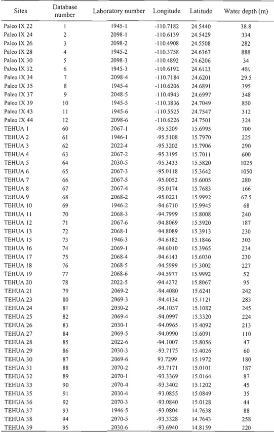
Table 2. Location of the surface sediment samples from the study of Kielt

(2006).

Database

Sites Laboratory number Longitude Latitude Water depth (m)

number Paleo IX 22 1 1945-1 -110.7182 24.5440 38.8 Paleo IX 24 2 2098-1 -110.6139 24.5429 334 Paleo IX 26 3 2098-2 -110.4908 24.5508 282 Paleo IX 28 4 1945-2 -110.3758 24.6367 888 Paleo IX 30 5 2098-3 -110.4892 24.6206 34 Paleo IX 32 6 1945-3 -110.6192 24.6123 401 Paleo IX 34 7 2098-4 -110.7184 24.6201 29.5 Paleo IX 35 8 1945-4 -110.6206 24.6891 395 Paleo IX 37 9 2048-5 -110.4943 24.6997 348 Paleo IX 39 10 1945-5 -110.3836 24.7049 850 Paleo IX 43 II 1945-6 -110.5525 24.7547 312 Paleo IX 44 12 2098:6 -110.6226 24.7501 324 TEHUA 1 60 2067-1 -95.5209 15.6995 700 TEHUA 2 61 1946-1 -95.5108 15.7970 225 TEHUA 3 62 2022-4 -95.3202 15.7906 290 TEHUA 4 63 2067-2 -95.3195 15.7011 600 TEHUA 5 64 2030-5 -95.3433 15.5820 1025 TEHUA 6 65 2067·3 -95.0118 15.3642 1050 TEH UA 7 66 2067·5 -95.0052 15.6005 280 TEHUA 8 67 2067-4 -95.0174 15.7683 166 TEH UA 9 68 2068-2 -95.0221 15.9992 67.5 TEHUA 10 69 1946-2 -94.67)0 15.9945 68 TEH UA Il 70 2068-3 -94.7999 15.8008 240 TEHUA 12 71 2067-6 -94.8069 15.5920 187 TEHUA 13 72 2068-1 -94.8089 15.3913 230 TEHUA 15 73 1946-3 ·94.6182 15.1846 303 TEHUAI6 74 2069-1 ·94.6010 15.3965 234 TEHUA 17 75 2068-4 -94.6143 15.6030 230 TEHUAl8 76 2068-5 -94.5999 15.3002 227 TEHUAI9 77 2068-6 -94.5977 15.9992 52 TEHUA 20 78 2022-5 ·94.4272 15.8067 95 TEHUA 21 79 2069-2 -94.4080 15.6241 242 TEHUA 23 80 2069-3 -94.4134 15.1121 283 TEHUA 24 81 2030-2 -94.1037 15.1082 245 TEHUA 25 82 2069-4 ·940997 15.3320 224 TEHUA 26 83 2030-1 -94.0965 15.4092 213 TEHUA 27 84 2069-5 ·94.0990 15.6091 110 TEHUA 28 85 2022-6 -94.1007 15.8056 47 TEHUA 29 86 2030-3 -93.7175 15.4026 60 TEHUA 30 87 2069-6 93.7299 15.1972 180 TEHUA 31 88 2070-2 ·93.7171 15.0101 187 TEHUA 32 89 2070-1 -93.3369 15.0164 87 TEHUA 33 90 2070-4 -93.3402 15.1202 45 TEHUA 35 91 2030-4 -93.0855 15.0849 35 TEHUA36 92 2070-3 -93.0840 15.0128 44 TEHUA37 93 1946-5 -93.0804 14.7638 88 TEHUA 38 94 2070-5 ·93.3328 14.7643 258 TEHUA 39 95 2030-6 -93.6940 14.8159 220

10

2. REGIONAL SETTING

2./ Oceanographie circulation

Primary productivity in the eastern tropical Pacifie is related to the dynamics of water masses, which are determined by atmospheric circulation patterns. The study area can be separated into two important zones: the area influenced by the California Current and the Tehuantepec Gulf (Figure 2).

1- California Bay and the western Mexican coast

The Northern limit of the area under the influence of the California CWTent is the Colorado River mouth in the Califomia Bay (USA) and the Southern limit is Corrientes Cape in the Mexican region of Sinaloa. From October to May, northwesterly winds induce surface circulation responsible for upwelling on the eastern margin of Califomia Bay and weak upwelling along the western Mexican coast (Barron et al., 2004), which is characterized by warm Tropical water masses (25 to 30°C) flowing southward. Upon reaching 10-20o_{N, they} shift seaward as the Southern branch of the North Pacifie subtropical gyre (Kessler, 2006). These waters are characterized by high oxygen concentration and 10w salinity (33-33.5) (Monreal-Gomez and Salas-de- Leon, 1998). However, because of the rarity of ocean data, the circulation of water masses is not completely understood during sununertime (Kessler, 2006).

2- Gulf of Tehuantepec

The Tehuantepec Gulf is occupied by warm subtropical waters (17 to 30°C), which are characterized by low nu trient concentration and salinity higher than 34.4 (Monreal-Gomez and Salas-de- Leon, 1998). From early winter to spring (December to May), the hydrology of this area is modulated by northerly strong seasonal winds (Tehuanos) formed in the Mexico Gulf blowing across Central America and passing trough the Isthmus of Tehuantepec (Boumaggard et al., 1998). When the winds reach the Pacifie Ocean, they drive intense upwelling in the northem part of Tehuantepec Gulf. Simultaneously, latitudinal shifts of the trade winds system and the Inteltropical Convergence Zone (ITCZ) are responsible for large anticyclonic and cyclonic eddies (Are llano-Tores et al., 2003; Monreal-Gomez and Salas-de­

Leon, 1998). These horizontal and vertical transports trigger the regional biological production by an enhanced nu trient supply. In summer, which is the tropical storms season, the Costa Rica CUITent extends along the coast before tuming westward near Corrientes Cape (Kessler, 2006).

2.2 Industrial development along the western Mexican coast

Human activities may severely affect the marine ecosystems with domestic and industrial wastewater discharged in the environment, as well as direct habitat destruction. Besides the urban development related to the fast growing of the populations in the western coastal areas of Mexico, the largest activities susceptible to cause harmful effects to the marine environment are the tourist resorts, harbours and oil-related industries. These activities are particularly thriving in the cities of Mazatlan, Puerto Vallarta, Manzanillo, Acapulco, Puerto Escondido, Puerto Angel and Satina Cruz (Ortiz-Lozano et al., 2005) (see figure 1).

12

...,' ~

~"

.

_.

_{,- ,}

/ .)NEC

-

-

.J

)

[2] / 1 1 ,. _:­ '•.l_'-.~ "=. fI'

~c

" :; '.:'I~ .1''';~

/

1....

~~

'. \:

Cal/famia Gu"

'i\

_, , '. ~

J?./

3-

.

.

-.

_..

~~~~

" NEC

..

,

...

.,.~ IlZC ~. '. ~ -...""",CRC

Figure 2. Surface ocean currents of the study area.

(1) Winter-Spring, (2) Summer-Fall. Red arrows correspond to Winter-Spring winds. Current abbreviations are: California CUITent (CC), Costa Rica Current (CRC), North Equatorial Current (NEC) and Intertropical Convergence Zone (ITZC)

3. MATERIAt AND METHODS

3. J Sampling

Surface sediments (0-1 cm) were sampled from box cores collected at water depths ranging from 24 to 1400 meters. Wet sediments were stored in a cool room (4°C) until palynological treatments and geochemical analyses. Sediment samples consist in sandy-silty mud and silty­ clayed mud.

Sediment mass accumulation rates at the most study sites are unknown. Nevertheless, analyses of 210_{Pb isotopes have shown that the sedimentation rate is about 0.035 to 0.05} cm·y(1 in La Paz Bay (Douglas et a1., 2001) and 0.05 ± 0.01 Cm-y(1 in Tehuantepec Bay (Are llano-Torres et a1., 2003; Ruiz-Femàndez et a1., 2004). Hence, if we assume similar sedimentation rates at our study sites, we may consider that the upper first centimetre of the box cores represent 20 to 30 years of accumulation on the sea-floor.

3.2 Geochemical analyses

Elemental and isotopie analyses have been performed on surface sediment samples from the Mexican margin exc1usively. Prior to geochemical analyses, sediments were dried, crushed with an agate mortar and homogenized. The total carbon (TC) and total nitrogen (TN) composition were determined on 5 to 8 mg of each sediment sample by high temperature combustion using a Carlo Erba™NC2500 elemental analyzer. Analyses of total inorganic carbon (TIC) were made by coulometry on dried and acidified sediments with 1N HCl by which carbonates were removed. Subtracting the total inorganic carbon from the total carbon yields the total organic carbon (TOC) content of a given sample. Replicated measurements of Organic Analytical Standard substances (Acetanilide, Atropine, Cyc1ohexanone-2, 4­ Dinitrophenyl-Hydrazone, Urea and five synthetic mixtures of soil) show a relative deviation of ± 0.1 % for the OC and ± 0.3% for TN. The analytical reproducibility corresponds to ± 5%.

Sediment samples for carbon isotopie analysis of organie matter were aeidified with 1N HC1, crushed and homogenized. Stable isotope data were obtained using a Carlo Erba™ elemental analyzer coupled to a GV Instmment IsoPrime™ mass spectrometer. Values were reported in

14 b-notation (%0) according to the international Vi enna-Pee Dee belernnite (VPDB) standard (Coplen, 1995). The bUC values were calibrated using two standards: DORM-2 (buC =

-28.50%0) and Leucine (b13C = -7.35%0) and yielded a relative deviation of ± 0.1 %0 (l cr) vs. V-PDB.

3.3 Palynological analyses

Surface sediment samples were prepared for palynological analyses according to the standardized laboratory procedures suggested by de Vernal et al. (1999). An aliquot of marker grains (Lycopodium c!avatum) was added to a volume of 5 cm3 of previously dried sediment. It was sieved with 10 and 106 ).lm screens to remove debris and particles superior to these size ranges. The fraction of sediment comprised between 10-106 ).lm was subsequently treated in alternation with hydrochloric acid (HCI 10%) and hydrofluoric acid (HF 48%) in order to dissolve carbonate, silicate and fluorosilicate minerais. The residual fraction of sediment was sieved again to eliminate particles smaller than 10 ).lm. Then, this residual material was deposed on a glycerin jelly and mounted for observation between a glass slide and a cover-slip.

In most samples, when the dinocyst concentration was sufficient, a mmlmum of 300 specimens were counted using an optical microscope at 400x to 1000x magnification. The concentrations of pollen grains, foraminifer organic linings and dinocysts were evaluated through the method of Matthews (1969) using the Lycopodium c!avatum spores and results are expressed as specimens per unit of dry sediment weight (specimens·g-'). According to de Vernal et al. (1987), the reproducibility of the counts is estimated to ± 10% at the 0.95 confidence interval. Dinocyst identification was made in conformity with the nomenclature of Rochon et al. (1999), Radi and de Vernal (2004) and Marret and Zonneveld (2003) (see systematics in Appendix C). Palynological treatments and counts in this study were made following the same procedures than the ones of Kielt (2006) in La Paz Bay and Tehuantepec Gulf. Therefore, both sets of data can be combined to establish a standardized database that includes 95 sites.

3.4 Statistical analyses

Statistical analyses were performed in order to quantitatively de termine which envirorunental variables are controlling the dinocyst abundance and distribution in surface sediments. A detrented correspondence analyse (DCA) was first achieved and revealed that the database follows a linear distribution. Therefore, a redundancy analysis (RDA\ was performed using the program CANOCO version 4.0 for Windows. RDA provides information about dinocyst assemblage responses to multiple envirorunental parameters and allows the determination of the level of influence corresponding to each particular parameter.

The analysis was carried out using the database of the coastal margin of Mexico that includes samples analysed herein in addition to data from Kielt (2006). Three species (Tuberculodinium vancampoae, Cyst of Protoperidinium americanum and Dubridinium spp.) occurring rarely and showing low relative abundances

«

4%) were not used for statistical analyses and sorne taxa grouping have been made in order to avoid possible bias in the identification between the two studies (Table 3). On the basis of their morphological similarities, cyst of Protoperidinium nudum were grouped with Selenopemphix quanta and Polykrikos kofoidii were grouped with Polykrikos cf. kofoidii. Similar intraspecific features bring sorne difficulties in separating Echinidinium delicatum, Echinidinium zonneveldiae and Echinidinium transparantum. Therefore, these species were grouped as Echinidinum transparantum. Echinidinium cf. granulatum and Echinidinium sp. x from the analyses of Kielt (2006), as weil as Echinidinium sp.l from this study, were grouped with Echinidinium spp. Finally, Spiniferites membranaceus and Spiniferites mirabilis were added to Spiniferites spp.

The environmental parameters retained for statistical analyses include temperature, salinity and productivity of surface waters (0 m) as weIl as the water depth and the distance to the shore of the sampling sites (Table 4).

• Productivity data

Productivity data from the Coastal Zone Color Scanner program (CZCS) (Antoine et al., 1996; Antoine and Morel, 1996) were calculated according to phytoplankton pigment

16

concentration based on sea-surface color satellite imagery. Uncertainties on the estimates are of the order of 17% (Antoine and Morel, 1996). We also used productivity data from the MODerate resolution Imaging Spectroradiometer (moDIS) program, which were calculated following the Vertical Generalized Primary Production Model (VGPM) developed by Behrenfeld and Falkowski (1997). Interpolations were carried out for sampling sites where productivity values were unavailable from these two datasets.

Comparison between productivity data extracted from the two different sources shows that moDIS-derived estimates of winter and annual productivity are significantly higher than data from the CZCS program. The largest heterogeneity appears in the area between 23°06'561 N and 20°38'471 N, where the difference between the two sensors reaches up to 150 g'Cm-2'y(1 in winter and to 380 g.c-m-2'y(1 for annual averages. These discrepancies may be explained by temporal changes in productivity from one decade to another since data acquisition with the CZCS and moDIS programs were made in 1978-1996 and 2002-2005, respectively; they can also be explained by the algorithms used to estimate productivity through the distinctive methods such as the differences between their respective data acquisition processes and period of observation (see discussion in Radi and de Vernal, 2008).

• Hydrographie parameters

Sea-surface salinity (SSS) and sea-surface temperature (SST) were extracted from the World Ocean Atlas (WOA, 2003) dataset published by the National Climatic Data Center (NCDC). The average values used here were calculated for a radius of 30 nautical miles at a depth of 0 meter. A radius of 60 nautical miles was used for 9 sites where measurements were too sparse.

Table 3. Dinocyst species reported

figure Il) and notes.

Dinocyst species PHOTOTROPHIC SPECIES Gonyaulacales Bileclalodinium spongium Lingulodinium machaerophorum Nemalosphaeropsis labyrinlhus Operculodinium cenlrocarpum Polyshaeridium zoharyi Spiniferiles delicalus Spiniferiles elongalus Spiniferiles membranaceus Spiniferiles mirabilis Spiniferiles ramosus Spiniferiles spp. Tuberculodinium vancampoae HETEROTROPHIC SPECIES Peridiniales Briganledinium spp.

Cyst of Penlapharsodinium dalei Cyst of Proloperidinium americanum Cyst of Proloperidinium nudum Echinidinium aculealum Echinidinium delicalum Echinidinium granulalum Echinidinium Iransparanlum Echinidinium spp. Lejeunecysla spp. Protoperidinioids Quiquecupsis concrela Selenopemphix nephroides Selonopemphix quanta Sielladinium spp. Voladinium spp. Gymnodiniales et Diplopsalidae Cyst of Gymnodinium calenalum Dubridiniurn spp. Polykrikos cf. kofoidii Polykrikos kofoidii Polykrikos schwarlzii Other Cyst A

III surface-sediment samples, abbreviations (cf.

Abbreviations BSPO LMAC NLAB OCEN PZOH SDEL SELO SMEM SMIR SRAM SSPP TVAN BSPP PDAL PAME PNUD EACU EDEL EGRA ETRA ESPP LSPP PERI QCON SNEP SQUA STSP VSPP GCAT DUBR PCKOF PKOF PSCH CYSA Notes

Grouped with Spiniferiles spp. Grouped with Spiniferiles spp.

Not included in statistical analyses

Not included in statistical analyses Grouped with S. quanla Grouped with E. Iransparantum

Grouped with Protoperidinioids Not included in statistical analyses

Not included in statistical analyses Grouped with P. kofoidii

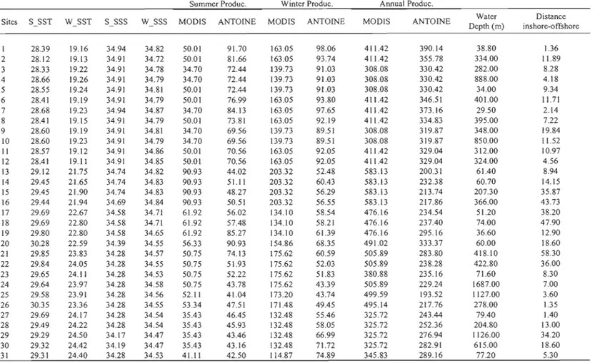
Table 4. Environemental parameters included in the statistical analyses corresponding to the database sampling sites:

summer and winter temperatures (S_SST and W_SST; oC), summer and winter salinities (S_SSS and W_SSS), summer,

winter and annual primary productivity estimated by moDIS and CZCS programs (gCm-2'y(i), the water depth (m) and the

distance inshore-offshore (km).

Summer Produc. Winter Produc. Annual Produc.

Sitcs S SST W SST S_SSS W SSS MODIS ANTOrNE MODIS ANTOINE MOOIS ANTOINE Water

Dcpth (m) Distance inshore-offshore 1 28.39 19.16 34.94 34.82 50.01 91.70 163.05 98.06 411.42 390.14 38.80 1.36 2 28.12 19.[3 34.91 34.72 50.01 81.66 163.05 93.74 411.42 355.78 334.00 Il.89 3 28.33 19.22 34.91 34.78 34.70 72.44 139.73 91.03 308.08 330.42 282.00 8.28 4 28.66 19.26 34.91 34.79 34.70 72.44 139.73 91.03 308.08 330.42 888.00 4.18 5 28.55 19.24 34.91 34.81 50.01 72.44 139.73 91.03 308.08 330.42 34.00 9.34 6 28.41 19.19 34.9[ 34.79 50.01 76.99 163.05 93.80 411.42 346.51 401.00 1l.71 7 28.68 19.23 34.94 34.87 34.70 84.13 163.05 97.65 411.42 373.16 29.50 2.[4 8 28.41 19.15 34.91 34.79 50.01 73.81 163.05 92.19 411.42 334.83 395.00 7.22 9 28.60 19.19 34.91 34.81 34.70 69.56 139.73 89.51 308.08 319.87 348.00 19.84 10 28.60 19.23 34.91 34.79 34.70 69.56 139.73 89.51 308.08 319.87 850.00 11.52 Il 28.57 19.12 34.91 34.86 50.01 70.56 163.05 92.05 411.42 329.04 312.00 10.97 12 28.41 19.11 34.91 34.85 50.01 70.56 [63.05 92.05 411.42 329.04 324.00 4.56 13 29.12 21.75 34.74 34.82 90.93 44.02 203.32 52.48 583.13 200.31 61.40 8.94 14 29.45 21.65 34.74 34.83 90.93 51.11 203.32 60.43 583.13 232.38 60.70 14.15 15 29.45 21.90 34.74 34.83 90.93 48.27 203.32 56.29 583.13 213.74 207.30 35.87 16 29.44 21.94 34.69 34.84 90.93 50.51 203.32 56.55 583.13 217.86 366.00 43.73 17 29.69 22.67 34.58 34.71 61.92 56.02 134.10 58.54 476.16 234.54 51.20 38.20 18 29.69 22.80 34.58 34.71 61.92 57.48 134.10 58.21 476.16 237.40 74.00 47.90 19 29.80 22.80 34.58 34.65 61.92 85.27 134.10 61.39 476.16 295.16 36.60 12.90 20 30.28 22.59 34.39 34.55 56.33 90.93 154.86 68.35 491.02 333.37 60.00 18.60 21 29.85 23.83 34.28 34.57 50.75 74.13 175.62 60.59 505.89 283.80 4[8.[0 58.30 22 29.84 24.05 34.28 34.55 50.75 51.93 175.62 52.03 505.89 238.28 422.80 36.00 23 29.65 24.11 34.28 34.53 50.75 52.22 175.62 51.83 380.88 235.16 71.60 8.30 24 29.64 23.97 34.28 34.58 50.75 43.78 175.62 43.39 505.89 229.24 1687.00 7.00 25 29.58 23.9[ 34.28 34.56 52.1 [ 41.04 173.20 43.74 499.59 193.52 1127.00 3.60 26 30.35 23.36 34.28 34.55 53.34 47.51 171.48 49.45 495.14 2[7.76 278.00 1.35 27 29.69 24.17 34.28 34.54 35.43 46.45 132.48 55.46 325.72 243.44 79.40 1.40 28 29.49 24.22 34.28 34.54 35.43 45.93 132.48 58.05 325.72 252.36 204.80 13.00 29 29.29 24.50 34.17 34.47 35.43 43.46 132.48 66.99 325.72 276.94 1126.00 34.20 30 29.32 24.42 34.19 34.47 35.43 43.16 132.48 71.72 325.72 282.91 615.00 18.60 3 [ 29.31 24.40 34.28 34.53 41.11 42.50 114.87 74.89 345.83 289.16 77.20 5.30 >-' 00

Sites S SST W_SST S_SSS W SSS MüDIS ANTürNE MüDIS ANTürNE MüDIS ANTürNE Depth (m) inshorc-offshore 32 29.46 25.14 34.06 33.98 34.52 42.71 68.82 57.75 209.23 251.00 587.60 8.43 33 29.46 25.55 34.03 34.34 34.52 40.84 68.82 52.58 209.23 226.10 67.40 0.66 34 29.44 25.52 34.52 34.31 34.52 43.33 68.82 5328 209.23 235.08 228.50 6.68 35 29.48 25.53 34.52 34.31 34.52 43.33 68.82 53.28 209.23 235.08 551.80 11.35 36 29.46 25.60 34.52 34.31 34.52 40.35 68.82 49.39 209.23 216.55 1188.00 23.82 37 29.50 26.15 33.85 34.35 39.24 41.39 74.21 52.30 255.58 210,84 61.30 4.10 38 29.49 26.16 33.85 34.35 39.24 41.39 74.22 52.30 255.58 210.84 102.60 7.50 39 29.55 26.50 33.85 33.76 39.24 46.22 74.22 59.44 255.58 232.17 96.60 2.70 40 29.51 26.40 33.85 33.76 39.24 46.22 74.22 59.44 255.58 232.17 191.20 8.90 41 29.40 26.92 33.85 33.93 34.10 47.69 47.96 55.39 178.67 219.55 58.50 1.80 42 29.39 26.90 33.85 33.87 34.10 47.69 47.96 55.40 178.67 219.55 362.30 9.10 43 29.64 27.19 33.60 34.18 35.85 43.46 57.44 40.22 198.65 188.28 713.90 29.40 44 29.61 27.18 33.60 34.18 35.85 43.46 57.44 40.22 198.65 188.28 428.90 23.20 45 29.63 27.13 33.47 34.18 35.85 44.03 57.44 42.61 198.65 198.89 92.80 8.10 46 29.76 27.12 33.14 34.18 35.85 47.60 57.44 40.67 198.65 202.28 36.50 5.40 47 29.84 27.43 33.14 34.36 35.85 44.81 57.44 38.80 198.65 181.53 63.40 4.29 48 29.91 27.45 33.14 34.36 35.85 44.81 57.44 38.80 198.65 181.53 173.40 10.36 49 29.83 27.45 33.14 34.36 3U5 44.81 31.12 38.80 127.92 181.53 883.10 14.65 50 29.85 27.37 33.14 34.36 31.15 43.90 31.12 39.62 127.92 181.09 995.10 25.80 51 29.68 27.43 33.14 34.28 34.07 47.62 41.42 46.50 157.67 199.45 153.00 5.90 52 29.64 27.40 33.14 34.26 34.07 47.62 41.42 46.50 157.67 199.45 73.00 3.20 53 29.66 27.41 33.14 34.08 41.23 47.15 58.09 43.82 188.81 187.75 58.90 1.50 54 29.58 27.59 33.14 33.93 41.23 54.65 58.09 45.76 188.81 195.65 24.00 0.20 55 29.55 27.58 33.14 33.97 41.23 54.65 58.09 45.77 188.81 195.67 79.80 2.10 56 29.62 27.56 33.14 33.98 41.23 47.15 58.09 43.82 188.81 187.75 241.40 9.45 57 29.69 27.75 33.14 33.95 41.23 47.82 58.09 49.37 188.81 190.91 51.50 5.07 58 29.96 27.88 34.00 34.00 41.84 56.55 64.24 45.64 201.60 213.40 72.60 2.00 59 29.72 27.90 34.00 34.01 41.84 56.29 64.24 47.30 201.60 219.07 70.10 1.00 60 29.42 26.31 33.53 34.20 46.99 71.78 160.02 75.08 384.29 342.75 700.00 27.70 H 29.43 26.29 33.53 34.20 46.99 76.24 160.02 76.48 384.29 354.74 225.00 17.50 62 29.34 26.35 33.69 34.19 46.64 77.32 143.18 78.75 349.88 362.24 290.00 23.90 63 29.28 26.39 33.69 34.18 46.64 74.40 143.18 77. 19 349.88 352.68 600.00 32.40 64 29.35 26.37 33.69 34.21 46.64 74.40 143.18 77.19 349.88 352.68 1025.00 43.50 65 29.26 26.20 33.92 34.27 46.78 71.83 166.51 75.21 345.00 342.09 1050.00 81.20 66 29.33 26.38 33.69 34.22 46.64 74.66 143.18 78.24 349.88 355.78 280.00 59.70 67 29.24 26.38 33.69 34.19 46.64 75.55 143.18 79.07 349.88 359.55 166.00 45.10 68 29.33 26.62 33.64 34.06 46.64 74.65 143.18 82.18 349.88 367.54 67.50 21.60 69 29.41 26.69 33.64 33.94 46.64 69.03 143.18 78.06 349.88 338.11 68.00 21.90 \Cl

SumrncrProduc. Wintcr Produc. Annual Produc.

Sites S_SST W_SST S_SSS W SSS MODIS ANTOfNE MOors ANTOfNE MODIS ANTOfNE Water

Depth (m) Distance inshore-offshore 70 29.32 26.38 33.64 34.18 46.64 68.88 143.18 76.17 349.88 331.02 240.00 45.60 71 29.24 26.40 33.64 34.24 46.64 67.53 143.18 75.09 349.88 326.64 187.00 68.50 72 29.21 26.29 33.92 34.32 46.78 64.37 166.51 71.67 345.00 311.42 230.00 91.00 73 29.41 26.04 33.92 34.35 46.11 55.46 133.80 65.38 296.09 275.80 303.00 109.00 74 29.27 26.43 34.00 34.27 46.78 60.33 166.51 68.97 345.00 291.38 234.00 85.80 75 29.25 26.48 33.64 34.23 46.64 63.80 143.18 72.83 349.88 308.57 230.00 64.70 76 29.15 26.39 34.00 34.48 46.78 58.36 166.51 68.18 345.00 285.97 227.00 96.20 77 29.41 26.67 33.64 33.88 46.64 64.45 143.18 75.33 349.88 320.17 52.00 20.20 78 29.38 26.29 33.92 33.98 45.86 61.04 143.18 70.30 258.66 266.03 95.00 37.40 79 29.29 26.81 33.64 33.78 44.61 54.43 70.02 65.14 206.18 269.92 242.00 55.20 80 29.56 26.71 33.64 33.97 45.00 48.39 85.32 60.03 219.18 246.15 283.00 108.00 81 29.55 26.85 33.64 3386 45.00 39.12 85.32 50.41 219.18 192.85 245.00 93.00 82 29.40 26.95 33.64 33.76 45.00 39.92 85.32 50.51 219.18 193.85 224.00 72.60 83 29.39 26.88 33.64 33.78 45.00 39.03 85.32 49.38 219.18 192.01 213.00 65.50 84 29.60 26.78 33.68 33.96 45.24 53.00 84.13 63.07 217.16 228.69 110.00 44.50 85 29.60 26.63 33.69 33.96 45.50 57.12 143.18 66.94 214.55 255.08 47.00 24.40 86 29.37 27.46 33.73 3392 46.69 36.38 85.32 42.77 219.18 141.46 60.00 41.30 87 29.68 27.24 33.78 33.67 45.00 33.71 85.32 38.82 219.18 145.83 180.00 23.00 88 29.94 27.20 33.78 33.56 45.00 36.41 85.32 42.07 219.18 158.60 187.00 74.70 89 29.95 27.66 33.78 33.48 56.40 41.87 46.35 39.44 190.58 157.39 87.00 45.80 90 29.55 27.69 33.78 33.49 56.40 41.87 46.35 39.44 190.58 157.39 45.00 37.80 91 29.40 27.75 33.77 33.51 55.78 43.51 46.35 40.42 190.58 165.06 35.00 22.30 92 29.40 27.76 33.78 33.49 56.40 45.89 46.35 40.48 190.58 196.55 44.00 28.90 93 30.34 28.11 33.77 33.45 55.18 43.85 46.35 42.85 190.58 223.72 88.00 46.40 94 29.95 27.73 33.78 33.45 56.40 43.74 46.35 44.12 190.58 176.16 258.00 67.40 95 29.78 27.46 33.56 33.58 45.00 38.68 85.32 46.23 219.18 177.30 220.00 88.00 N o

4. RESULTS

4.1 Geochemical data

Throughout the study area, percentages of total organic carbon (TOC) in sediment are relatively high and range from 0.25% to 5.08%. TOC shows higher values with increased distance to the shore and depth (Figure 3B-C). Elemental analyses performed on surface sediments show C:N ratios ranging from 5.35 to 15.44, except for station 59 which has a value of 22.74 (Figure 3A). Carbon isotope signatures (8 13 Carg) increase with the distance to the shore and depth, and are of the order of -21.02% to -25.91 %, WitJl most of the values comprised between -21 % and -23.5 % (Figure 3A-B-C) (Table 5). Both TOC and 813C indicate higher contribution of marine fluxes offshore likely related to lesser terrigenous inputs and lower sedimentation rates.

4.2 Palynomorph assemblages

Palynomorph assemblages are characterized by terrestrial (pollen grains) and manne components (foraminifer organic linings and dinocysts) with higher concentrations of marine microfossils throughout the study area (Figure 4).

Dinocyst concentrations calculated from dry weight of sediment are highly variable (from 66 to 55 620 cysts·g·l) and follow a latitudinal gradient with highest values in the Northem part of the study area and a decreasing trend toward the Tehuantepec Gulf (Figure 5, Tables 6-7). Concentrations in our study area are high in comparison with the concentrations observed in the coastal zones of North America north of 400

N (e.g. Radi et al., 2007; Pospelova et al., 2008) and reflect high planktonic productivity. Otherwise, observations from sites located in Tehuantepec Gulf are consistent with the results ofVasquez-Bedoya et al. (2008).

Concentrations of organic linings are of the order of ~ 65 to 34 000 linings'g'l (see table 6-7). These values are high comparatively to those reported from other studies (e.g. Pospelova et al., 2008; Thibodeau et al., 2006; Hamel et al., 2002). Since foraminifer organic linings represent a fragrnentary picture of the biocenoses, their abundant content suggests very high benthic productivity. Analyses of benthic foraminifera shells versus linings are also used as

22

proxy for carbonate dissolution in sediments (de Vernal et al., 1992). In La Paz Bay, higher lining concentrations contrast with a low number of forarninifer shells, reflecting dissolution processes in sediments. On the contrary, shell vs. lining ratios in the Northern part of Tehuantepec Gulf suggest that calcium carbonate in sediments from that region are well­ preserved (e.g. Kielt, 2006).

Pollen grain concentrations are highly variable with values ranging from ~216 to 64736 pollens'g- ' (see tables 6-7). Low terrestrial palynomorph concentrations were recorded in La Paz Bay and along the Mexican margin, whereas the Northern part of Tehuantepec Gulf shows maximal values.

Ratios of dinocyst to pollen grains are often used as "continentallity" index (e.g., de Vernal and Giroux, 1991). Values are comprised between 0.05 and 3.29 along the Mexican margin and Tehuantepec Gulf and the lowest ratios are observed in the Northern palt of Tehuantepec Gulf and at station 59 (0.05 and 0.07) (see tables 6-7). Sites from La Paz Bay show dominant dinocyst concentrations with ratios reaching up to 7.78.

4.3 Dinocyst assemblages

With a total of 34 taxa identified, dinocyst assemblages show a large diversity of dinocyst species, notably among heterotrophic ones (Figures 6-7). The abundance and good preservation of the observed Protoperidinium and Echinidinium cysts, in spite of their extreme sensitivity to oxidation processes (Zonneveld et al., 2001) indicate a good preservation of organic matter and dinocysts in sediment.

Bitectatodinium spongium and Brigantedinium spp. are abundant ail along the coast and correspond together to more than 40% of the assemblages. Heterotrophic taxa are likely to dominate in upwelling zones with Brigantedinium spp., Selenopemphix quanta, Polykrikos kofoidii and Echinidinium species. In addition, the upwelling area of Tehuantepec Gulf is marked by a high occurrence of the phototrophic taxon Polysphaeridium zoharyi. In opposition, most phototrophic taxa including Bitectatodinium spongium and Spiniferiles spp. principally occur in regions which are not under the influence of upwelling.

Several sites are characterized by the presence of cysts of harmful taxa such as Polysphaeridium zoharyi, cyst of Gymnodinium catenatum and Lingulodinium machaerophorum. While the main zone of occurrence of P. zoharyi is observed in the Northern part of Tehuantepec Gulf (Figure 8A), the distribution of

L.

machaerophorum is scattered among the study sites, notably between Mazatlan and Puerto Vallarta (Figure 8B). Due to their poor state of preservation in several slides, cysts of Gymnodinium catenatum were not counted. This species appears fragmented most of the time, which makes the quantification of its occurrence in sediment difficult (Plate 1). G. catenatum has been reported in bloom events implicating massive shrimp mortalities along the western Mexican coast (Alonso-Rodrfguez, 2003). Unfortunately, the poor preservation of the cysts III

sediments does not permit their use for analysing dinocyst distribution in relation to hydrographical conditions and therefore identifying parameters favourable to HABs related to G. catenatum blooms.

4.2 Statistical analyses

Redundancy analysis further provides insight into the relationship between dinocyst distribution and environmental parameters. The first two axes explain respectively 43.7% and 29.4% of the total variance. Although the absence of a strong correlation between individual taxa and the first two axes, sorne hydrographical parameters are likely to play a role in the geographical distribution of the dinocyst assemblages (Tables 8-9-10). The nearshore­ offshore gradient is strongly linked to the first axis (R = 0.7336), whereas annual, winter and summer productivity and winter salinity correlate with axis 2 (R= 0.689, 0.569, 0.616 and 0.616). Echinidinium transparantum is in the negative domain of axis 1. Otherwise, axis 2 shows a relation with the relative abundance of heterotrophic taxa (R2 = 0.75394) (Figure 9) and is characterized by an opposition between Spiniferiles de/icatus on the positive side and heterotrophic taxa in the negative side of the ordination (Figure 10).

The sample scores for axes 1 and 2 in the ordination diagram illustrate different regional groupings. Here, four assemblages are weil defined and the similarities between assemblages from sites located in upwelling areas are clearly shown (Figures 11-12):

24

• Assemblage 1 corresponds to the upwelling zone of La Paz Bay. This assemblage is characterized by high dinocyst concentrations and its composition is dominated by heterotrophic-related taxa such as Polykrikos kofoidii, Eehinidinium aeuleatum, Eehinidinium granulatum and Brigantedinium spp.

• Assemblage 2 represents the coastal zone comprised between the California Bay and Tehuantepec Bay where human activities are developing rapidly. Total cyst concentrations follow a decreasing trend, with highest values between Mazatlàn and Manzanillo and lower values towards the Tehuantepec Gulf. Heterotrophic species Polylcrikos kofoidii, Eehinidinium spp. and Brigantedinium spp. largely dominate. Moreover, Bileetatodinium spongium is present in higher proportions.

• Assemblage 3 is restricted to the Northern part of the Tehuantepec Gulf, where seasonal upwelling results in high primary productivity. This area is however marked by low dinocyst concentrations, high Polysphaeridium zoharyi occurrence and relatively high proportions of Spiniferiles spp.

• Assemblage 4 is associated to the Southern part of the Tehuantepec Gulf, which is not under the influence of upwelling and which is characterized by a low productivity. Dinocyst concentrations and the ratios of heterotrophic to autotrophic species show the lowest values. This assemblage is dominated by Bileetatodinium spongium, Spiniferiles spp. and Brigantedinium spp. Finally, Spiniferiles delieatus exhibits in this zone its greatest relative abundance.

station .: 20 ₅₉ ._ - . 0 - - ­ '5

~

.

,

.

" , l ' ." 10 •

.

" ", .,' '" ",

.

'.' " _{~ ~} :z

o

ü o 1­ ü ~ 0.,1 • 0,1 1 • [DI -22t" ..,

.'

' . ·21 .'

.

·22 ·21

. .

'.

_'.

R2: 0.4041

2l

·22 J .' .' R2=0095 -22 marine Algae

. .

·23 ·2'

..

..

.'

.,

.

.

.'

-24" • 0 23 _1-.:.:~

.

-231.', •

..

, ,

,

_24 1 ' • ' " -23 ·24 ·26 /;(

""

_.

-""

:.r

.26 1" -/;( K,

•

• .261L!'!­ _ _... ~ ..J /;( K, _.'

.

_, N·W , S·E o '0 10 JO 40 50 60 0 500 1000 1500 2000 10 15 20 25

Laliludinal gradient Distance to the shore (km) Depth (m) C:N

f3

C

Figure 3. Spatial distribution of C:N, TOC (%) and

o

of sediments from the Mexican margin. (A) C:N ratios and

isotopie composition oforganic carbon (ol3C) vs latitudinal gradient, (B) Percentages of total organic carbon (TOC)

and 013C vs the distance to the shore, (C) TOC and Ol3C vs depth, (D) Ol3C vs C:N ratios.

Data are not available for La Paz Bay and Tehuantepec Gulf.

N VI

26

." c::

.=

o

..

,;; <fi c: 0 ~ m ë x ~ ~ u c: _i: 0 _0. U <fi Cl e Vi c: c: Vi .Q Ci Ü <fi

~

V> _{0 N} c: _§ ~ .r::; c: 0 u .~ §. ~ ë 0. Cl 2;­ .~ ë m <li ~ _.;; u c: ë

'"

c: Cl X ;; (; ~ ~ _{~ U} ~ 8 u -0 c: => => c:~ _~- i: 0. u u 0 8 .~.~

"'-

0. _<Ji e :-='0) ₀ 0. à:

(ij _{>- .} 'en Cl v> C:. _<fi <il

c: ~ >- _{ro ro} N

uv> c: _Ë Cl u

0 -_{c:~ ~o "'~} m c: Q; 0 _c: c: => :> c: v> v>

Ci :ç; Qi c: c:

ëi~ 0 . 8 u..= :c ëi <t <t

&

&

N-W ]0000 1) IY:JOOoo ..moo 200 1 100 0 ~(J() .• 1.1 ~-l 1 1 '---J La Paz Bay . ~_ ._ _UPWELLING Mexlcan Margln UPWELLING Mexican Margin UPWELLING S-E Figure 4. Dinocyst concentrations (cysts.g-I), pollen grain concentrations

(grains.g- '), foraminifer organic lining concentrations (Iinings.g- '), heterotrophic to phototrophic taxa ratios, dinocysts to pollen grains ratios, annual productivity estimated by moDIS program, annual productivity estimated by CZCS program and sample scores of axes 1 and 2 from redundancy analysis.

Table 5. Elemental and isotopic analyses, depth and distance to

the shore of surface-sediment samples of this study.

Distance to

Sites TC TIC TOC TN C:N B13 _{C Depth}

the shore (%) (%) (%) (%) (m) (km) 13 2.34 0.66 1.68 0.17 11.55 61.40 8.94 14 2.67 1.03 1.65 0.20 9.76 60.70 14.15 15 2.91 1.09 1.82 0.27 7.83 207.30 35.87 16 7.26 2.18 5.08 0.73 8.11 366.00 43.73 17 2.96 2.62 0.34 0.07 5.35 51.20 38.20 18 3.92 2.17 1.75 0.25 8.02 74.00 47.90 19 1.83 0.25 1.59 0.17 10.78 36.60 12.90 20 2.45 0.56 1.89 0.20 10.94 60.00 18.60 21 6.49 1.80 4.69 0.67 8.19 418.10 58.30 22 6.20 0.78 5.43 0.68 9.33 422.80 36.00 23 9.61 9.50 0.11 0.11 1.13 71.60 8.30 24 3.17 0.52 2.65 0.32 9.81 1687.00 7.00 25 2.42 0.37 2.05 0.23 10.25 1127.00 3.60 26 1.65 0.22 1.43 0.15 11.24 278.00 1.35 27 2.06 0.74 1.32 0.18 8.46 79.40 1.40 28 3.43 0.36 3.08 0.36 9.88 204.80 13.00 29 3.67 0.40 3.27 0.38 10.03 1126.00 34.20 30 5.44 0.80 4.63 0.57 9.54 615.00 18.60 31 1.63 0.60 1.03 0.10 12.33 77.20 5.30 32 3.40 0.89 2.51 0.33 8.96 587.60 8.43 33 2.00 0.25 1.75 0.16 13.03 67.40 0.66 34 3.74 0.63 3.11 0.37 9.91 228.50 6.68 35 4.47 0.88 3.60 0.43 9.75 551.80 11.35 36 1.93 0.19 1.74 0.19 10.41 1188.00 23.82 37 1.55 1.26 0.29 0.06 5.58 61.30 4.10 38 1.97 0.54 1.43 0.17 10.06 102.60 7.50 39 2.22 0.79 1.43 0.18 9.18 96.60 2.70 40 2.95 0.75 2.20 0.29 8.70 191.20 8.90 41 1.42 0.46 0.96 0.10 10.98 58.50 1.80 42 3.40 1.10 2.31 0.32 8.42 362.30 9.10 43 2.99 0.54 2.46 0.30 9.51 713.90 29.40 44 3.12 0.41 2.71 0.32 9.90 428.90 23.20 45 4.48 2.00 2.49 0.19 15.44 92.80 8.10 46 2.21 1.02 1.19 0.15 8.93 36.50 5.40 47 1.85 1.14 0.71 0.12 7.15 63.40 4.29 48 2.89 0.79 2.10 0.27 8.96 173.40 10.36 49 2.01 0.64 1.37 0.18 8.71 883.10 14.65 50 2.25 0.35 1.90 0.22 10.08 995.10 25.80 51 3.13 0.82 2.31 0.28 9.50 153.00 5.90 52 1.99 0.42 1.57 0.14 12.63 73.00 3.20 53 1.71 0.62 1.10 0.09 13.78 58.90 1.50 54 1.67 0.58 1.09 0.11 11.07 51.50 5.07 55 1.74 0.59 1.15 0.16 8.21 24.00 0.20 56 2.43 0.68 1.75 0.23 8.97 79.80 2.10 57 1.59 0.38 1.21 0.12 11.73 241.40 9.45 58 3.09 0.49 2.60 0.31 9.64 72.60 2.00 59 4.88 1.54 3.34 0.17 22.74 70.10 1.00

28

(

\

c

\

~~/

Dinocyst concentrations (cysts-g-') ~)60 000 .-" () 30000 ~; 5000