PROCEEDINGS OF SPIE
SPIEDigitalLibrary.org/conference-proceedings-of-spie
The adaptive optics simulation
analysis tool(kit) (AOSAT)
Feldt, M., Hippler, S., Cantalloube, F., Bertram, T.,
Obereder, A., et al.
M. Feldt, S. Hippler, F. Cantalloube, T. Bertram, A. Obereder, H. Steuer, O.
Absil, M. Le Louarn, "The adaptive optics simulation analysis tool(kit)
The adaptive optics simulation analysis tool(kit) (AOSAT)
M. Feldt
a, S. Hippler
a, F. Cantalloube
a, T. Bertram
a, A. Obereder
b, H. Steuer
a, O. Absil
c, and M. Le
Louarn
da
Max Planck Institute for Astronomy, Königstuhl 17, D-69117 Heidelberg, Germany
bJohann Radon Institute, Altenberger Straße 69, A-4040 Linz, Austria
c
Planetary & Stellar systems Imaging Laboratory, Université de Liège, Allée du 6 Août, 19C - Bât.
B5c, B-4000 Liège 1, Belgium
d
European Southern Observatory, Karl-Schwarzschild-Str. 2, D-85748. Garching, Germany
ABSTRACT
AOSAT is a python package for the analysis of single-conjugate adaptive optics (SCAO) simulation results. Python is widely used in the astronomical community these days, and AOSAT may be used stand-alone, integrated into a simulation environment, or can easily be extended according to a user’s needs. Standalone operation requires the user to provide the residual wavefront frames provided by the SCAO simulation package used, the aperture mask (pupil) used for the simulation, and a custom setup file describing the simulation/analysis configuration. In its standard form, AOSAT’s "tearsheet" functionality will then run all standard analyzers, providing an informative plot collection on properties such as the point-spread function (PSF) and its quality, residual tip-tilt, the impact of pupil fragmentation, residual optical aberration modes both static and dynamic, the expected high-contrast performance of suitable instrumentation with and without coronagraphs, and the power spectral density of residual wavefront errors.
AOSAT fills the gap between the simple numerical outputs provided by most simulation packages, and the full-scale deployment of instrument simulators and data reduction suites operating on SCAO residual wavefronts. It enables instrument designers and end-users to quickly judge the impact of design or configuration decisions on the final performance of down-stream instrumentation.
Keywords: Adaptive Optics, Simulation, Design, Performance Evaluation
1
INTRODUCTION
Adaptive optics (AO), with its capabilities to correct optical disturbances caused by Earth’s atmosphere in real time, is becoming ever more common in visible/infrared astronomy. Increasingly seen as a standard facility that supports any type of standard instrumentation, so-called single-conjugate AO (SCAO) is inherently part of a large number of next-generation projects currently in one of their pre-commissioning phases (METIS;1 MICADO;2HARMONI;3NFIRAOS;4
GMT;5for an overview see Hippler et al. 20196). In these phases, the design of SCAO systems relies heavily on end-to-end simulations, the typical end-to-end-to-end-to-end (SC)AO simulation package such as YAO,7 COMPASS,8OOMAO,9or CAOS10 provides a few numbers that characterize the system’s performance during the simulation, plus the residual wavefronts at each time step. The numbers provided are typically the Strehl ratio, a single measure for the quality of an optical image, plus its variation across wavelengths, and according to separation from the AO reference star. For modern high-performance instrumentation these numbers are not sufficient to judge the performance effectively, and a deeper analysis of the residual wave fronts is required. AOSAT currently performs in-depth analyses of residual wavefronts focusing on different aspects such as (but not limited to) high-contrast imaging, the impact of fragmented pupils, and non-common path aberrations. AOSAT is on the one hand an integrated tool, capable of providing a summary "tearsheet" of the system performance from a given simulation output, on the other hand built in a modular fashion so that it can easily be extended with additional "analyzers" focusing on the user’s area of interest. This paper describes the software, its purpose and design principle, how to obtain, install, use, and extend AOSAT, and the various analyses being performed in the current implementation.
Further author information: (Send correspondence to M. Feldt) M. Feldt: E-mail: [email protected], Telephone: +49 6221 528 262
2
PURPOSE AND DESIGN
Many sophisticated (SC)AO simulation packages exist, and are used for a variety of purposes: Instrument development and design is a key use case, but fundamental research and application in laboratory setups is also among the applications of such software. Most such packages produce a set of key numbers as output, the Strehl number being the most prominent one among these, plus the residual phases at each end-to-end simulation step. Unsurprisingly, all of the information is in the residual phase data (getting them as close to zero as possible being the whole purpose of adaptive optics), from which also all the numbers can be re-computed.
Analyzing the residual phases is in most cases done by the same people who executed the simulation, often by means of custom, on-the-fly-written scripts. This is sufficient in e.g. project work towards a specific goal, but it makes comparisons between projects difficult. Different simulation software, different key metrics examined, and different definitions of key metrics occur across the AO landscape, and custom tailored analysis solutions can routinely only comply to one specific set of requirements and definitions.
AOSAT is intended to provide a standardized platform that can analyze the output of many if not all SCAO simulation packages by feeding residual phases, the telescope pupil and a set-up file describing fundamental simulation parameters. On output, AOSAT provides a well-tested and standardized set of analyses with a well-documented set of metrics and graphical tools to have an insight in the AO correction quality. AOSAT can be easily extended with custom-made additional analyzers. The "analyzer" object is an independent analysis tool focused on one particular aspect of the wavefront, of which many already exist in AOSAT, but more can be contributed. Thanks to its modular architecture described below, AOSAT can be easily receive inputs (residual phase screens) from any AO simulator
2.1
Design - Setup File
In addition to the residual phase screens and the telescope pupil, the main input required by AOSAT is the set-up file. This file must contain the parameters used for the AO simulation, as detailed in the documentation.11
To run AOSAT one needs to provide
1. phase screens generated by a proper end-to-end simulation tool in FITS*12 files in a subdirectory of your current
working directory.
2. the telescope pupil. It, too, must be stored in a FITS file, and the scale in pixels per metre and its overall dimensions must naturally be the same as for the residual phase screens. AOSAT operates with transmission numbers, so if your 2D pupil map contains a 1.0 at a given location, it is transparent, whereas if it contains a 0.0 it is opaque. Intermediate values are welcome, i.e. the pupil map can also contain non-binary values representing transmission variations (e.g. the effect of segmented primary mirrors or apodizing masks).
3. the set-up file describing key properties, such as the pixel scale, the unit in which residual phases are given, the simulation frequency, and the wavelength at which the analysis is desired. In addition there are parameters that describe the organization of the input files, and certain switches that can be set according to the user’s discretion. AOSAT can handle a multitude of file and frame ordering schemes, most of them simultaneously. Given a target directory and filename pattern
screen_fpattern = '*residual_phase*.fits'
AOSAT will read all files matching the pattern. They will be sorted in a somewhat intelligent way according to integer numbers found in the filenames. If certain or all individual files contain cubes of data along the NAXIS3 of the FITS file, such frames will be served sequentially one after the other as individual phase screens. AOSAT relies on the phase screens having an equal temporal spacing throughout the sequence reflected in the loopfreq key in the set-up file. Note that AOSAT is not inherently intended to analyze single phase screens, but most individual analyzers that do not focus on some temporal aspect can be set up to do so.
A typical full set-up file looks as follows:
*Flexible Image Transport System. Most simulation tools do or can easily produce this type of output which is simple-structured,
human readable and flawlessly implemented in just about every astronomical piece of software. There is no plan to ever support HDF5. If you want to know why, look athttps://cyrille.rossant.net/moving-away-hdf5/
pupilmask = 'telescope_pupil.fits'
screen_dir = 'residual_phasescreens'
screen_fpattern = '*residual_phase*.fits'
ppm = 10.0 # pixels pr metre
loopfreq = 1000.0 # Hz - actually it's the frequency of phase screens on disk
phaseunit = "micron" # unit of phase screens
an_lambda = 3.0e-6 # analysis wavelength in metres
2.2
Design - Serving Frames
For flexibility, finding, sorting, reading, unit conversion and potentially zero-padding the input residual phases is decoupled from the actual analyses. A so-called frameserver handles these tasks, and hands the residual phases one by one to the individual analyzers. In this way, not only can different output formats (single frame files, cubes of frames, flexible numbering scheme) be used with AOSAT, but it is also possible to replace the frameserver with a custom one that can e.g. read different file formats, or serve frames directly out of a simulation code. For quick test runs, the frameserver can also be directed to skip certain frames, or serve only a subset of a temporal sequence.
2.3
Design - Analyzing Tools
For reasons of flexibility, every analysis to be performed has its own analyzer object in AOSAT. In general, these objects do not require dedicated parameters in the set-up file, other than if they are required to run or not. The choice to not require such parameters has been made in order to keep results comparable and reliable. There are however a few exceptions to this rule (currently there is exactly one exception: The contrast analyzer can be set up to run either non-coronagraphic, or with an ideal coronagraph).
The deliberate design choice to keep all analyses independent of each other does cause some overheads, e.g. some FFTs are performed multiple times as there is no communication between analyzers. However it facilitates implementing new analyzers at ease. To do so, there is a base class dmy_analyzer from which new analyzers can be derived and its methods overwritten. For details, see the documentation on readthedocs.11
During a run, each analyzer gets served the input residual phases one at a time, plus the information on how many frames to expect in total. Once serving is finished, each analyzer provides a finalize() method that needs to be called in order to perform concluding computations such as, of course, statistics over all frames. After that, analyzers expose the results of the individual analysis in question via dedicated properties, and all internal ones provide the convenience methods make_report()and make_plot().
For detailed description of available standard analyzers, and the way that analyses are actually performed, see Sec.4
3
INSTALLING AOSAT
3.1
Installation
1. Make a new empty directory, e.g. like this:
$ mkdir AOSAT $ cd AOSAT
2. Clone the repository
$ git clone https://github.com/mfeldt/AOSAT.git
3. Create and activate a virtual environment (if you don’t know/have virtualenv, use pip to install it)
$ virtualenv -p python3.6 venv $ source venv/bin/activate
(This assumes using bash, there’s also venv/bin/activate.csh and a few others) 4. Change to the repository and install:
$ cd AOSAT
$ python setup.py install
That’s it, python should install the package and all required dependencies!
3.2
Verifying the Installation
To verify that the installation is fine, you can do the following: 1. run the test suite
$ python setup.py test
2. Try the individual files
$ cd src/aosat $ python fftx.py $ python aosat_cfg.py $ python util.py $ python analyze.py
Ideally everything should terminate without failures. Beware it may take a while.
3.3
Documentation
When following the installation instructions an examples directory is checked out along with the code. To find the examples, you can do the following in python (running of course, in your activated AOSAT environment):
>>> import os
>>> os.path.join(os.path.split(aosat.__file__)[0],'examples')
In the examples directory, you will find a number of set-up files that can be adapted to your needs by changing the relevant parameters. You may also start with the minimum example given above in Sec.2.1. In order to do more than runnig the examples, the best way is of course to look at the documentation which is available fromhttps://aosat.readthedocs.io. Here, you will find detailed descriptions of the setup files, the configuration of a particular analysis, and the outputs that AOSAT provides when a particular analysis is performed.
4
STANDARD ANALYZERS
4.1
"Tearsheet" Functionality
A common use case is to produce a so-called “tearsheet”, a double-sided page summarizing the most interesting performance indicators from the results of a given AO simulation.
This can be achieved easily for the provided close-loop example like so:
>>> import aosat
>>> example_path = os.path.join(os.path.split(aosat.__file__)[0],'examples')
>>> example_file = os.path.join(example_path,'example_analyze_closed_loop.setup')
>>> aosat.analyze.tearsheet(example_file)
This will produce two files in the current working directory:
ts_test.txt ts_test.pdf
Guess what the familiar extensions mean and look at them with the appropriate tool for each to see what they are about. An example can be seen in Fig.1.
������������ ��������������� ������������������������������� ���������������������������� ���������������������������� ���������������������������� ��������������������������� ������������������������������ �������������������������� ������������������������� ���������������������������� ������������������������������������������������������������������������� ����������������������������� ���������������������������� ������������������������������������������������������������������������� ����������������������������������������������������������������� ������������������������������ ���������������������������� ���������������������������� �������������������������������������������� ������������������������������������������������������ ������������������������������������������������������������������������� ��������������������������������������� ������������������������� ������������������������� ������������������������������������ ��� � ��� �������� ��� ��� ��� � ��� ��� ��� ��������� ���������������� ��������������� ������������������� ������������������ ������������������������������������������� ��� ��� ��� ��� ��� ��� ��� ��� ��������� �� �� � �� �� ����� �� �� � �� �� ����� ����� ����� ����� ����� ����� ����� ����������� ����������� �������������������������������� ���������������������������������� � ����� ����� ����� ����� ���� ���� ���� ���� ����� ����� ����� ���������� � ���� ����� ����� ����� ��������� ��� �� �� �� � �� �� �� ����������������������������� ������������������������ ��� ��� ��� ��� ��� ��� ��������������� ��� ��� ��� ��� ��� ��������������� ���������������� �������������������������� �� ���� ����������������� ��������������������������� ��������������������������������� ��� � ��� ��� ��� ��� � ��� ��� ��� ����������������� ��� ��� ��� ��� ��� ��� ��� ��������� ��������������������������������������������������� �
Figure1. Example tearsheet output of AOSAT.
4.2
The PSF Analyzer
Analyzing the PSF (Point Spread Function) is done in a straight forward way: the residual phase of stored in each screen is transformed into a PSF by means of the well known:
np.abs(fftForward(aperture*np.exp(1j*phase)))**2
where aperture represents the telescope entrance pupil defined in the setup file. A number of additional performance indicators are calculated on both the resulting PSF, and the input phase. This can e.g. reveal deviations from the Maréchal approximation when certain types of aberrations (e.g. waffle modes) occur. Such double computations are carried out for
• the Strehl ratio is measured on the AO residual phase 𝜑 as 𝑆 = 𝑒−𝜎2𝜑.
• the Strehl ratio is measured on the PSF as 𝑆 = 𝐼𝑝𝑒𝑎𝑘/𝐼𝑟𝑒𝑓,𝑝𝑒𝑎𝑘, where 𝐼 is the PSF’s intensity distribution, and 𝐼𝑟𝑒𝑓
is the intensity distribution of a reference PSF resulting from a perfectly flat wavefront.
• the tip and tilt excursion of the PSF is measured on the phase 𝜑 by means of a least squares fit of a tilted flat wavefront to the phase
• the tip and tilt excursion of the PSF is measured on the PSF by means of fitting a 2D Gaussian to the core of the PSF. 4.2.1 Plot caption
Figure2. Typical Figure produced by the PSF analyzer.
When called on its own, or on a figure with sufficient available subplot space, frg_anaylzer.makeplot() will produce a figure as shown in Fig.2. The suggested caption for the figure could be:
Resulting time-averaged PSF in units of peak intensity. Additionally shown is the Strehl ratio derived from the peak intensity, denoted as “SR(PSF)”, and derived from the wavefront quality, denoted as “SR(WF)”. The tip-tilt statistics are shown in the lower part, also derived from the PSF directly as well as from the wavefronts. 𝑄90means that 90% of TT
excursions are smaller than the quoted value. 4.2.2 Resulting properties
psf_analyzerexposes the following properties after psf_analyzer.finalize() has been called:
Table1. psf_analyzer properties
Property type Explanation
psf 2D ndarray (float) Time-averaged PSF.
strehl float Strehl ratio of PSF derived from peak intensity. sr_wf float Strehl ratio of PSF derived from residual wave fronts. ttx 1D ndarray (float) of length
n_frames
Global tip for each frame from Gauss-fitted PSF location (mas).
tty 1D ndarray (float) of length n_frames
Global tilt for each frame from Gauss-fitted PSF location (mas).
ttilt 1D ndarray (float) of length n_frames
Global excursion from centre, determined from wavefront (mas)
ttjit float rms of ttilt
ttq90 float 90% quantile of ttilt
ttjit_psf float rms of√︀ttx2+ tty2
4.3
Pupil Fragmentation Analyzer
The fragmentation analyzer looks, as the name implies, at pupil fragments individually. Pupil fragments are sections of the telescope pupil that are not connected to one another and thus form individual fragments or “islands”. Fragmentation may occur due to the secondary support structure (aka "spiders"), or by design of having several disconnected primary mirrors on a single support structure. Spiders can cause the additional inconvenience of the low-wind effect (see below).
This fragmentation can give rise to two kinds of effects in adaptive optics, the
Island effect arises when the AO loop itself introduces independent piston terms for each fragment due to the reconstructor’s inability to provide accurate information on the wavefront’s piston offset across the spider. The other possibility is the
Low-wind effect originally dubbed “Mickey Mouse effect” due to the shape of the PSF it produces, it occurs at very low wind speeds at ground level. Here, a physical phase difference between adjacent fragments exists due to the air being cooler on the downwind side of the radiatively cooled spider. This causes a phase jump across the spider, plus frequently a tilt across the affected downwind fragment as temperatures re-equilibrize further down the weak flow (see e.g. Fig. 1 in13). Again combined with the reconstructor’s inability to yield accurate piston information, these do not get corrected.
The result of both is similar (apart from the possible fragment tilt caused by the low-wind effect), but it is important to note that the first is purely due to missing information, while the second has a physical origin. Few AO simulations accurately simulate the low-wind effect correctly, it usually needs to be introduced specifically.
In any case tip-tilt terms remain closely connected to pupil fragmentation, as a global tilt across the pupil will also cause piston terms of fragments to differ, particularly along the tilt gradient. Vice versa, a real piston difference of fragments opposing each other in the pupil (may) appear as a global tilt.
4.3.1 Finding fragments
Analyzing pupil fragments is an integral part of AOSAT, the fragments are thus identified during the setup of any analysis run, no matter which particular analyzer is used afterwards. Fragments are found by means of thescipy.ndimage.label function, and are contained in the setup dictionary’s fragmask element.
Figure3. Labeled apertures of some well-known telescopes / projects.
4.3.2 Analyzing fragments
At each time step, frg_analyzer determines the piston and tip-tilt terms of each individual fragment. Piston and fragmental (i.e. global across the fragment) tip-tilt is determined by a least squares fit of a tilted but otherwise flat plane to the wavefront inside the fragment.
for i in range(num_fragments):
## tilt from WF
## wfrag contains the valid indeces for each fragment
C,_,_,_ = np.linalg.lstsq(self.A[i], frame[self.wfrag[i]]) self.ttxt[self.ffed,i] = C[0]
self.ttyt[self.ffed,i] = C[1] self.pistont[self.ffed,i] = C[2]
Piston, tip, and tilt of each fragment are stored for each time step.
Upon completion, i.e. when finalize() is called, the analyzer computes the mean, and the standard deviation on each of the stored time series.
4.3.3 Plot captions
Figure4. Plots produced by the pupil fragmentation analyzer.
When called on its own, or on a figure with sufficient available subplot space, frg_anaylzer.makeplot() will produce two figures like as shown in Fig.4. The figure caption for the left image would be:
Pupil fragmentation analysis. The color image gives the piston and tilt of the frame with the largest span of piston values across fragments during the last 19% (xx s) of the sequence. The numbers in the fragments give the piston value standard deviation (in nm) across the full sequence for the corresponding fragment.
Note the length of the sequence to search for the worst piston occurrence can be altered by use of the tile argument in the call of frg_analyzer.finalize(tile=0.8).
The figure caption for the right image would be: Piston term of individual pupil fragments over time
4.3.4 Resulting properties
frg_analyzerexposes the following properties after frg_analyzer.finalize() has been called:
Table2. frg_analyzer porperties
Property type Explanation
piston 1D ndarray (float) of length n_fragments
Array holding the mean piston value for each pupil fragment (in nm).
dpiston 1D ndarray (float) of length n_fragments
Array holding the standard deviation of the piston value for each pupil fragment (in nm).
pistont 2D ndarray (float) of shape (n_frames, n_fragments).
Array holding individual piston values for each frame in the sequence.
ttx 1D ndarray (float) of length n_fragments
Array holding mean tip deviation for each fragment (in mas).
dttx 1D ndarray (float) of length n_fragments
Array holding the standard deviation of tip deviation for each pupil fragment (in mas).
ttxt 2D ndarray (float) of shape (n_frames, n_fragments)
Array holding individual tip values for each frame in the sequence.
tty 1D ndarray (float) of length n_fragments
Array holding mean tilt deviation for each fragment (in mas).
dtty 1D ndarray (float) of length n_fragments
Array holding the standard deviation of tilt deviation for each pupil fragment (in mas).
ttyt 2D ndarray (float) of shape (n_frames, n_fragments)
Array holding individual tilt values for each frame in the sequence.
pistframe 2D ndarray (float) Frame holding the worst piston pattern across the top (1-attr:tile) (see below) part of the simulated sequence. tile float Fractional tile above which the analyzer looks for the
worst piston frame in the sequence.
4.4
Zernike Expansion
zrn_analyzeryields the time averaged Zernike expansion of the individual residual phase frames. The average, and the standard deviation of each term are calculated and presented.
Basis generation The number of Zernike terms each residual wavefront is expanded into is determined by the zterms key in the setup file.
The function called to set up the basis is poppy.zernike.arbitrary_basis() from the poppy package14. If you want to set up
your own basis to expand wavefronts into, you should create a numpy (cupy) array of shape (d,d,nterms), where 𝑑 is the pupil diameter of your aperture array in sd['tel_mirror'] (seesetup file). Each plane needs to contain a phase map of the corresponding basis term. All non-zero pixels in the aperture must be covered by the basis, else the analyzer will crash. This array should be inserted into the setup dictionary key zernike_basis.
sd = aosat.analyze.setup()
sd['zernike_basis'] = my_basis_array
a = aosat.analyze.zrn_analyzer(sd)
Note the order of these statements which is crucial for the result to be as expected. Of course your own basis does not necessarily need to be a basis of type Zernike.
Wavefront expansion The expansion of individual wavefronts itself is done by aosat.util.basis_expand(), which computes the cross-correlations between the wavefront and individual basis terms.
4.4.1 Plot captions
Figure5. Plot produced by the Zernike analyzer.
When called on its own, or on a figure with sufficient available subplot space, aosat.analyze.frg_anaylzer. makeplot()will produce a figure like shown in Fig.5. The caption would be:
Time-averaged Zernike expansion of residual wavefronts. The blue line denotes the average amplitude of each term, the shaded area ranges from the average plus one standard deviation to the average minus one standard deviation.
Reading this section you have probably noticed that the zrn_analzer is somewhat mis-labeled as “Zernike” analyzer, since the functionalities to create the basis, and to expand the wavefront is actually outside of the analyzer. The only core functionality currently is to restrict the basis choice to Zernike, and produce the plot/report.
4.4.2 Resulting Properties
aosat.analyzers_.zrn_analyzer exposes the following properties after aosat.analyzers_. zrn_analyzer.finalize()has been called:
Table3. zrn_analyzer properties
Property type Explanation
modes 1D float NDarray of length zterms Time averaged mean amplitude of each mode dmodes 1D float NDarray of length zterms Standard deviation of each mode amplitude modest 2D float NDarray of shape (zterms,
nframes)
Individual modal expansion for each frame
4.5
Residual Phase
phs_analyzer is actually more a decorative displayer of the last residual phase frame than an actual analyzer. Nevertheless, it tracks the rms of each input phase frame and computes the mean rms in the end.
4.5.1 Plot caption
Figure6. Plot produced by the residual phase analyzer.
When called on its own after aosat.analyze.phs_analyze.finalize(), aosat.analyze. phs_analyze.make_plot()will produce a plot as shown in Fig.6. The caption would read:
Last residual wavefront in nm. The number in the center gives the time-averaged rms of the residual wavefront. 4.5.2 Resulting properties
After calling aosat.analyze.phs_analyze.finalize(), phs_analyzer will expose the following properties:
Table4. phs_analyzer properties
Property type Explanation
rms float mean RMS of all wavefronts in nm.
rmst 1D NDarray of length n_frames individual rms of all residual phase frames in nm lastphase 2D array Last residual phasescreen (in nm)
4.6
Temporal Variance Contrast
4.6.1 MotivationHigh-contrast performance is one of the prime metrics to judge the quality of closed-loop operation of AO systems these days. Thus, a contrast curve must not be missing from any decent analysis tearsheet for a given AO simulation. In addition, a kind of quick-look at focal plane residuals after removing the part of the PSF which is purely due to entrance pupil diffraction can reveal ultimate contrast limitations and underlying causes such as the actuator geometry or a wind-driven halo.15
The prime motivation to come up with TVC (Temporal Variance Contrast) was the following list of requirements: Computing the TVC should allow to
1. be able to quickly access the contrast of a large set of simulations (hundreds) that produced a large number of residual WF frames (thousands) each.
2. not have to rely on specific assumptions about position in the sky, amount of field rotation, ADI (Angular Differential Imaging) algorithm used, etc.
3. assess essentially the impact of a given deterioration of wavefront quality, rather than predict the precise contrast value.
No. 1 inhibits the use of a full-fledged analysis software like such as VIP16 (https://github.com/vortex-exoplanet/VIP) coupled to a full model of the wavefront propagation through the coronagraphic optical train as realized by the HEEPS17 package., which usually runs a couple of hours on each simulation output. We needed something much simpler and faster. No. 2 fostered the idea of coming up with a measure that attempts a measurement of those limitations that any angular differential imaging (ADI)18 algorithm would be unable to overcome. This has only partly been achieved, but the
underlying thoughts are: Static aberrations cause static PSF patterns, which are easy to handle and cause little or no noise. Aberrations that are de-correlated between frames cause independent realizations of random PSF patterns, these can essentially not be overcome by ADI methods (But instead average out to a certain degree over time). That leaves aberrations that change in intermediate time-scales for the ADI algorithms to handle. These, however, are hardly present in many simulations as SCAO simulation packages ususally do not simulate NCPA (Non-Common Path Aberrations) variations, flexure, pupil shifts, or any other slowly-changing effect yet.
So in order to measure the fundamental limit imposed by the independent realizations, we came up with the idea of looking at the variance along the temporal axis at each image location separately. This is nicely independent of any assumed amount of field rotation, which would not change these statistics. As variance can be computed in an on-line fashion on focal-plane frames being computed one-by-one subsequently, the method is suitable to operate on very large data sets that cannot be held in memory entirely. Since we are not heavily interested in the absolute contrast value, we operate on single pixels only rather than averaging over a certain aperture.
4.6.2 Definition
For this section, we compute a comparison between TVC and a standard ADI contrast. We use a simulation data set from the METIS (Mid-Infrared ELT Imager and Spectrograph)1preliminary design phase.
We define two types of contrast to compare, in addition to the actual HCI† result. First the TVC. It is computed in the following way:
1. Compute image frames from the residual phases and stack in a cube 2. Compute the variance 𝑉 along the temporal axis for each pixel
3. For a given separation, average the variances over an annulus covering that separation 4. Compute the 5𝜎 contrast for that separation as 5 ×
√ ¯ 𝑉
In order to have a simplified‡model for ADI, we compute what we will call the ADI contrast in the following way
1. Compute image frames from the residual phases and stack in a cube
2. Compute a robust mean image along the temporal axis, robust meaning we exclude the 10% of values furthest from the median in each temporal vector.
3. Subtract the above image from each frame 4. Average along the temporal axis
5. For a given separation, compute the variance 𝑉 of pixel values over an annulus covering that separation 6. Compute the 5𝜎 contrast for that separation as 5 ×√𝑉
Note that when the assumption works that the temporal variance is a good measure for the variations that cannot be overcome by the ADI algorithm, the TVC contrast and the ADI contrast computed in this way should be related by the square root of the number frames. This is because the ADI procedure averages along the temporal axis, and the error of the mean (found in the spatial standard deviation when ADI contrast is measured) should be given by the temporal standard deviation divided by the square root of the number of independent realizations.
†
High-Contrast Imaging, using a full-fledged ADI package to analyze the simulated data.
4.6.3 Comparison to ADI
In order to compare the various methods to measure contrast, we computed the TVC and the above simplified ADI model on the same residual phase cube that was used to derive the contrasts in the METIS PDR (Preliminary Design Review).
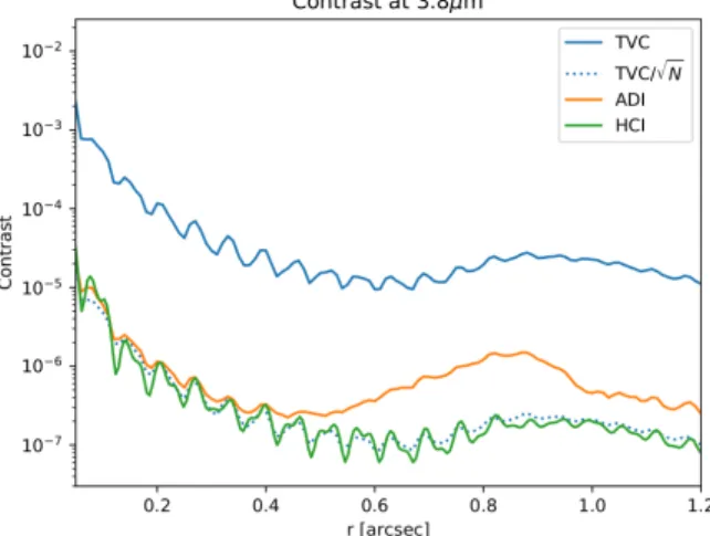
Figure7. Contrast curves measured on METIS’1standard HCI data set. The green curve is the actual ADI result obtained by running VIP16on the resulting image cube. The straight blue line represents the ADI contrast measured with the method defined in Sec.4.6.2.
The dotted blue line is the same divided by the square root of the number of frames in the cube. The orange curve represents our simplified ADI model, also defined in Sec.4.6.2
Fig7shows the contrast curves derived in the various ways. Two observations can be made. Firstly, the match of the TVC curve divided by the square root of the number of frames to the contrast curve measured by true ADI via the VIP package is excellent. This said, we have to add two notes of caution here:
Firstly, we are working on simulated data and the detailed comparison has been made on one particular instance only. More in-depth analysis is needed, and ultimately it may be of great interest to perform a similar comparison on real data from a high-contrast imaging instrument.
Secondly, the input for this experiment is sampled at 300 ms steps, all frames are completely de-correlated from one another. For continuous simulation data sampled at much higher frequency, tvc_analyzer tries to determine the correlation length of a given input cube, and divide by the number of independent realizations instead of the number of frames in order to predict final 1hr ADI contrast. If this determination goes wrong for any reason, results will be unreliable!
The temporal statistics do not vary with time in these simulations - the TVC contrast measured on 500 frames is the same as the one measured on the full set of 12,000 frames. Thus, if the condition of independent frames and no mid-temporal-frequency being present in the system is granted, the analysis can be greatly accelerated by running only on a subset! Secondly, the simplified ADI model matches the scaled TVC and the measured ADI curve only partly. While the match in the interesting region around 5𝜆/𝐷 is reasonable, the curves diverge around the control radius. It is beyond the scope of this comparison to investigate the details of this behaviour.
4.6.4 Impact of wavefront quality
Figure8. Evolution of contrast versus wavefront quality.
While the prediction of the actual high-contrast performance is nice-to-have, the prime goal of a contrast analysis in AO simulations is to catch all factors that have a pronounced impact on the high-contrast performance of the system.
In order to investigate this, we deteriorated the wavefronts by multiplying residual phase screens with a factor. The impact on contrast at 5𝜆/D can be seen in Fig.8. TVC and modeled ADI contrast as defined in Sec.4.6.2behave nicely in parallel. TVC appears to be slightly less impacted than the ADI model, but not to a level larger than the usual uncertainties of contrast loss predictions. We conclude, that we can safely use our TVC analyses to find critical impacts on contrast with this method.
4.6.5 tvc_analyzer
tvc_analyzeris different from most other analyzers in AOSAT as it can run in two distinct mode: Coronagraphic and non-coronagraphic. This is selected during instantiation by means of the ctype keyword:
a = tvc_analyzer(sd,ctype='icor') # run with an ideal coronagraph inserted
a = tvc_analyzer(sd, ctype='nocor') # run without coronagraph
a = tvc_analyzer(sd) # run without coronagraph
When running in coronagraphic mode, the PSF creation from each residual phase frame is routed through a ideal coronagraph as described in Cavarroc et al. (2005).19 In this case, the incoming complex amplitude 𝐴 (represented as tel_mirror * exp(1j*phase)) is modified to ¯𝐴 = 𝐴−Π, where Π represents the telescope pupil. The usual factor of a square root of Strehl√𝑆 is not implemented in tvc_analyzer, as Strehl is either so high that it’s negligible, or the determination of 𝑆 is unreliable. Thus the implementation is tel_mirror * exp(1j*phase) - tel_mirror. In addition, tvc_analyzer produces an additional plot by default when instantiated in coronagraphic mode: The ideal coronagraphic PSF.
4.6.6 Plot captions
When called on its own in coronagraphic mode, or on a figure with sufficient available subplot space, tvc_anaylzer. makeplot()will produce two figures like shown in Fig.9
The figure caption for the left image would be :
Resulting contrast curves. The black curve shows the PSF profile, the red curve the resulting5𝜎 contrast from temporal variation of the PSF. The green curve shows the predicted contrast limit achievable in an integration of 1 hr after ADI processing.
Figure9. Plots produced by the temporal variance contrast analyzer.
Time-averaged coronagraphic PSF. Intensities are relative to the peak of the non-coronagraphic PSF.
In the non-coronagraphic case, the right figure is missing. The green curve is plotted only if a successful determination of the correlation time could be achieved.
4.6.7 Resulting properties
tvc_analyzerexposes the following properties after finalize() has been called:
Table5. tvc_analyzer properties
Property type Explanation
ctype str type of coronagraph (“icor” or “nocor”)
mean 2D ndarray time-averaged PSF.
variance2 2D ndarray variance2[1] contains the non-coronagraphic time-averaged PSF (icor only)
contrast 2D ndarray 5 sigma contrast of the PSF
rcontrast 2D ndarray raw contrast, i.e. the normalized PSF.
rvec 2D ndarray (float) Image where each pixel contains distance to centre (mas) cvecmean 2D ndarray (float) Mean TVC contrast at locations in rvec.
cvecmin 2D ndarray (float) Minimum TVC contrast at locations in rvec. cvecmax 2D ndarray (float) Maximum TVC contrast at locations in rvec. rvecmean 2D ndarray (float) Mean raw contrast at locations in rvec. rvecmin 2D ndarray (float) Minimum raw contrast at locations in rvec. rvecmax 2D ndarray (float) Maximum raw contrast at locations in rvec. corrlen float Measured correlation length [#frames] max_no_cor float Peak intensity of non-coronagraphic PSF
4.7
Spatial Power Spectrum
The power spectrum analyzer derives the time-averaged spatial power spectrum of the residual phase frames. 4.7.1 Anti-aliasing
The spatial power spectrum is derived by an FFT of the input residual phase:
fftArray = np.fft.fftshift(np.fft.fft2(ps*mask,norm='ortho'))
fftArray = (fftArray * np.conj(fftArray)).astype(np.float)
The mask deployed here is an apodized version of the input pupil. The apodization avoids ringing, i.e. the appearance of Airy-ring-like structures in the power spectrum. Apodization is achieved by modifying the input telescope pupil mask in three steps:
2. apodize the binary mask by applyingskimage.morphology.binary_dilation3 times to derive 3 versions of the pupil, each 1 pixel smaller than the previous one.
3. The 1 pixel wide border region which makes the difference between successively dilated pupils is assigned a transmission value according to a Gaussian fall-off.
Figure10. Pupil apodization. Left: crop of the original telescope pupil, in this case of the ELT showing a representation of the segmentation. Center: Same crop of the pupil after “binarization”. Right: Apodized pupil applied to residual phase to avoid aliasing/ringing.
Currently there is no parameter to vary the number of steps for the apodization. In case you absolutely want to, you’d have to assign the mask manually like so:
>>> import aosat
>>> nsteps = 6 # let's say you want 6 steps for a really soft pupil
>>> a=aosat.analyze.sps_analyzer()
>>> a.mask = util.apodize_mask(a.sd['tel_mirror'] != 0,steps=nsteps)
The resulting power spectra are averaged azimuthally, and finally temporarily. 4.7.2 Plot captions
When called on its own mode, or on a figure with sufficient available subplot space, make_plot() will produce a figure as shown in Fig.11. The figure caption would be:
time-averaged spatial power spectrum of the residual wavefronts. For comparison, the red line shows the expected open-loop Kolmogorov spectrum. The blue line represents a von Kármán spectrum for an outer scale of𝐿0= 25 m.
Note that the blue line is plotted only, when the L0 key is present in thesetupdictionary 4.7.3 Resulting properties
sps_analyzerexposes the following properties after finalize() has been called:
Table6. sps_analyzer properties
Property type Explanation
mask 2D ndarray (float) Apodization mask generated from pupil f_spatial 1D ndarray (float) Spatial frequency vector [1/m]
ps_psd 1D ndarray (float) Power spectral density at f_spatial [nm^2/m^-1]
5
Conclusions
We have presented AOSAT, a python package for the analysis of SCAO end-to-end simulation residual phase screens, a represnettaion of the telescope pupil and the AO parameters of the simulation. In its standard configuration, it provides a set of performance indicators and informative graphs to assess the quality of the AO correction. We have shown how AOSAT may be used stand-alone, integrated into a simulation environment, or can easily be extended according to a user’s needs. Additionally we discussed the internal workings of the included standard analyzers of AOSAT.
We hope that this package will not only produce high quality analyses for the future of our own METIS project, but will also be useful for others and perhaps even allow some comparisons between projects.
ACKNOWLEDGMENTS
AOSAT originated from a set of on-the-fly written scripts exactly as criticized in Sec.2. These scripts were used to analyze the SCAO simulation done for phase B of the METIS1project.
Numerous people in this project and at ESO have discussed these analyses when presented at FDR, and thus contributed to the idea of producing a coherent analysis package that will in turn produce reliable, reproducible analyses for later phases, and possibly other projects, too.
REFERENCES
[1] Bertram, T., Absil, O., Bizenberger, P., Brandner, W., Briegel, F., Cantalloube, F., Carlomagno, B., Vázquez, M. C. C., Feldt, M., Glauser, A. M., Henning, T., Hippler, S., Huber, A., Hurtado, N., Kenworthy, M. A., Kulas, M., Mohr, L., Naranjo, V., Neureuther, P., Obereder, A., Rohloff, R.-R., Scheithauer, S., Shatokhina, I., Stuik, R., and van Boekel, R., “Single conjugate adaptive optics for METIS,” in [Adaptive Optics Systems VI ], Close, L. M., Schreiber, L., and Schmidt, D., eds., 10703, 357 – 367, International Society for Optics and Photonics, SPIE (2018).
[2] Clénet, Y., Bernardi, P., Chapron, F., Gendron, E., Rousset, G., Hubert, Z., Davies, R., Thiel, M., Tromp, N., and Genzel, R., “SAMI: the SCAO module for the E-ELT adaptive optics imaging camera MICADO,” in [Adaptive Optics Systems II], Ellerbroek, B. L., Hart, M., Hubin, N., and Wizinowich, P. L., eds., 7736, 1326 – 1338, International Society for Optics and Photonics, SPIE (2010).
[3] Neichel, B., Fusco, T., Sauvage, J.-F., Correia, C., Dohlen, K., El-Hadi, K., Blanco, L., Schwartz, N., Clarke, F., Thatte, N. A., Tecza, M., Paufique, J., Vernet, J., Louarn, M. L., Hammersley, P., Gach, J.-L., Pascal, S., Vola, P., Petit, C., Conan, J.-M., Carlotti, A., Vérinaud, C., Schnetler, H., Bryson, I., Morris, T., Myers, R., Hugot, E., Gallie, A. M., and Henry, D. M., “The adaptive optics modes for HARMONI: from Classical to Laser Assisted Tomographic AO,” in [Adaptive Optics Systems V ], Marchetti, E., Close, L. M., and Véran, J.-P., eds., 9909, 92 – 106, International Society for Optics and Photonics, SPIE (2016).
[4] Herriot, G., Hickson, P., Ellerbroek, B., Andersen, D., Davidge, T., Erickson, D., Powell, I., Clare, R., Gilles, L., Boyer, C., Smith, M., Saddlemyer, L., and Véran, J., “Nfiraos: Tmt narrow field, near-infrared facility adaptive optics - art. no. 62720q,” Proceedings of SPIE - The International Society for Optical Engineering 6272 (07 2006).
[5] Lloyd-Hart, M., Angel, R., Milton, N. M., Rademacher, M., and Codona, J., “Design of the adaptive optics systems for GMT,” in [Advances in Adaptive Optics II ], Ellerbroek, B. L. and Calia, D. B., eds., 6272, 115 – 126, International Society for Optics and Photonics, SPIE (2006).
[6] Hippler, S., “Adaptive Optics for Extremely Large Telescopes,” Journal of Astronomical Instrumentation 8, 1950001– 322 (Jan. 2019).
[7] Rigaut, F., “yao, a monte-carlo simulation tool for adaptive optics (ao) systems,” (2012).
[8] Ferreira, F., Gratadour, D., Sevin, A., and Doucet, N., “Compass: An efficient gpu-based simulation software for adaptive optics systems,” in [2018 International Conference on High Performance Computing Simulation (HPCS) ], 180–187 (2018).
[9] Conan, R. and Correia, C., “Object-oriented Matlab adaptive optics toolbox,” in [Adaptive Optics Systems IV ], Marchetti, E., Close, L. M., and Véran, J.-P., eds., 9148, 2066 – 2082, International Society for Optics and Photonics, SPIE (2014).
[10] Carbillet, M., Camera, A. L., Folcher, J.-P., Perruchon-Monge, U., and Sy, A., “The software package CAOS 7.0: enhanced numerical modelling of astronomical adaptive optics systems,” in [Adaptive Optics Systems V ], Marchetti, E., Close, L. M., and Véran, J.-P., eds., 9909, 2194 – 2200, International Society for Optics and Photonics, SPIE (2016).
[11] Feldt, M. and Hippler, S., “AOSAT Documentation.” Readthedocs,https://aosat.readthedocs.io(2020). (Accessed: 11 November 2020).
[12] “Fits standard document.”https://fits.gsfc.nasa.gov/fits_standard.html(1993). Accessed: 2020-08-12.
[13] Sauvage, J.-F., Fusco, T., Lamb, M., Girard, J., Brinkmann, M., Guesalaga, A., Wizinowich, P., O’Neal, J., N’Diaye, M., Vigan, A., Mouillet, D., Beuzit, J.-L., Kasper, M., Louarn, M. L., Milli, J., Dohlen, K., Neichel, B., Bourget, P., Haguenauer, P., and Mawet, D., “Tackling down the low wind effect on SPHERE instrument,” in [Adaptive Optics Systems V], Marchetti, E., Close, L. M., and Véran, J.-P., eds., 9909, 408 – 416, International Society for Optics and Photonics, SPIE (2016).
[14] Perrin, M., Long, J., Douglas, E., Sivaramakrishnan, A., Slocum, C., and others, “POPPY: Physical Optics Propagation in PYthon,” (Feb. 2016).
[15] Cantalloube, F., Farley, O. J. D., Milli, J., Bharmal, N., Brandner, W., Correia, C., Dohlen, K., Henning, T., Osborn, J., Por, E., Suárez Valles, M., and Vigan, A., “Wind-driven halo in high-contrast images. I. Analysis of the focal-plane images of SPHERE,” A&A 638, A98 (June 2020).
[16] Gonzalez, C. A. G., Wertz, O., Absil, O., Christiaens, V., Defrère, D., Mawet, D., Milli, J., Absil, P.-A., Droogenbroeck, M. V., Cantalloube, F., Hinz, P. M., Skemer, A. J., Karlsson, M., and Surdej, J., “VIP: Vortex image processing package for high-contrast direct imaging,” The Astronomical Journal 154, 7 (jun 2017).
[17] Delacroix, C., “Heeps: High-contrast end-to-end performance simulator,” (2020).
[18] Marois, C., Lafrenière, D., Doyon, R., Macintosh, B., and Nadeau, D., “Angular Differential Imaging: A Powerful High-Contrast Imaging Technique,” ApJ 641, 556–564 (Apr. 2006).
[19] Cavarroc, C., Boccaletti, A., Baudoz, P., Fusco, T., and Rouan, D., “Fundamental limitations on Earth-like planet detection with extremely large telescopes,” Astronomy and Astrophysics 447, 397–403 (Feb. 2006).