HAL Id: hal-01997698
https://hal.insa-toulouse.fr/hal-01997698
Submitted on 29 Jan 2019
HAL is a multi-disciplinary open access
archive for the deposit and dissemination of
sci-entific research documents, whether they are
pub-lished or not. The documents may come from
teaching and research institutions in France or
abroad, or from public or private research centers.
L’archive ouverte pluridisciplinaire HAL, est
destinée au dépôt et à la diffusion de documents
scientifiques de niveau recherche, publiés ou non,
émanant des établissements d’enseignement et de
recherche français ou étrangers, des laboratoires
publics ou privés.
Characterization of the cutting phenomenon in orbital
drilling of titanium alloys (TiAl6V4)
P. A. Rey, Johanna Senatore, Yann Landon
To cite this version:
P. A. Rey, Johanna Senatore, Yann Landon. Characterization of the cutting phenomenon in orbital
drilling of titanium alloys (TiAl6V4). 11th International Conference on High Speed Machining, Sep
2014, Prague, Czech Republic. �hal-01997698�
ISSN 1803-1269 (Print) | ISSN 1805-0476 (On-line) Special Issue | HSM 2014
11th International Conference on High Speed Machining
September 11-12, 2014, Prague, Czech Republic
HSM2014-00000
CHARACTERIZATION OF THE CUTTING PHENOMENON IN ORBITAL
DRILLING OF TITANIUM ALLOYS (TIAL6V4)
P.A .Rey, K .Moussaoui, J. Senatore, Y. LandonInstitut Clément Ader (ICA) Université de Toulouse ; INSA, UPS, Mines Albi, ISAE Bât 3R1, 118 route de Narbonne, F-31062 Toulouse Cedex 9, France.
*P.A. Rey; pierre-andre.rey@univ-tlse3.fr
Abstract
The orbital drilling is a complex operation. Due to the tool trajectory, which is helical, chip thickness is highly variable. This is why the cutting forces are very difficult to estimate.
The aim of this study is to determinate influence of tool geometry and cutting conditions on cutting force and to determinate the final quality of the machined hole. At first, the geometry of the chip is modeled taking into account the parameters defining the trajectory and the tool. A cutting force model based on the instantaneous chip thickness is then set up. An experimental part validates the cutting force model through measures of cutting force made during orbital drilling tests. Another experimental part is made. A series of drilling by varying the geometry of the tool is realized. During all these drillings, cutting forces will record using the Kistler dynamometer. And then a dimensional measure will be realized on all holes using a three-dimensional measuring machine.
Using cutting force model and the results of tests, it is possible to conclude on the influence of the tool geometry, on the hole geometry. And so it's possible to optimize these parameters in order to increase the final quality of the hole.
Keywords:
Orbital drilling, TiAl6V4, tool geometry, cutting forces,
1 INTRODUCTION
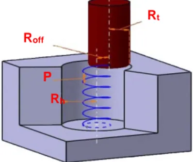
The orbital drilling, also called helical milling, is a process notably used in the aeronautical industry. It is very different from the axial drilling. It consists in machining a hole with a tool which has a smaller diameter, driven on a helical trajectory (Figure 1).
This process is used especially because it generates low cutting forces [Lutze, 2008]. As a consequence, the burr formation at the entry and at the exit of the hole is largely reduced, and also the risk of delamination when drilling composite materials is highly reduced. [Denkena and al.,
2008] [Brinksmeier et al., 2008]. Operations such as cleaning or deburring are then considerably reduced. For the cutting force model in orbital drilling, three approaches are possible: the numerical approach, the analytical and the semi analytical approach. The numerical approach used in the work of Lorong [Lorong et al, 2002] aims to simulate chip formation by a finite element study. Analytics approaches as Merchant’s model Merchant, 1945] or Oxley’s model [Oxley, 1989] consist to describe the most physically possible the cutting phenomenon in order to calculate the cutting forces. The semi-analytics approaches, also called mechanistic approaches, are the most used one to calculate machining cutting forces and particularly when the process is complex [Fontaine, 2004], like helical milling. This approach is based on analytics approaches by simplifying all the parameters of the tool geometry or of the tool/workpiece couple by a constant experimentally defined with calibration test.
2 MODELING OF ORBITAL DRILLING
2.1 Geometrics settings of the orbital drilling
In order to be able to develop a model of the chip geometry, the input data of the model and the references that are necessary to form the equation, need to be previously defined.
P Roff
Rt
Rh
MM Science Journal | Special Issue | HSM 2014
The defining data of the tool’s geometry:
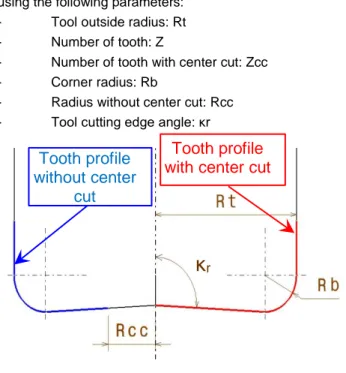
The global tool geometry (Figure 2) is generically defined using the following parameters:
- Tool outside radius: Rt - Number of tooth: Z
- Number of tooth with center cut: Zcc - Corner radius: Rb
- Radius without center cut: Rcc - Tool cutting edge angle: κr
Cutting’s parameters:
In order to determine the chip thickness, it is necessary to define the cutting parameters. The tool feed, along helical trajectory, can be decomposed in an axial feed fa and a tangential feed ft.
Drilling radius: Rh
Interpolation radius, called offset: Roff= Rh – Rt Pitch (mm): P
Cutting speed (m/min): Vc Axial feed (mm/rev): fa Tangential feed (mm/rev): ft Axial feed per tooth: f_za=f_a/Z Tangential feed per tooth: f_zt=f_t/Z
References definition: Hole center to drill: HL
Machine’s reference: this reference is fixed. 𝑹𝑹𝒎𝒎= (𝑯𝑯𝑯𝑯, 𝑿𝑿, 𝒀𝒀, 𝒁𝒁)
Orbital reference: this reference permit to define the tool’s positions « i » on the helical trajectory.
𝑹𝑹𝒐𝒐𝒐𝒐= (𝑯𝑯𝑯𝑯, 𝑿𝑿𝒐𝒐𝒐𝒐, 𝒀𝒀𝒐𝒐𝒐𝒐, 𝒁𝒁)
With: � 𝑿𝑿𝒐𝒐𝒐𝒐= 𝑐𝑐𝑐𝑐𝑐𝑐 𝜃𝜃𝑖𝑖. 𝑿𝑿 + 𝑐𝑐𝑠𝑠𝑠𝑠 𝜃𝜃𝑖𝑖. 𝒀𝒀 𝒀𝒀𝒐𝒐𝒐𝒐= −𝑐𝑐𝑠𝑠𝑠𝑠 𝜃𝜃𝑖𝑖. 𝑿𝑿 + 𝑐𝑐𝑐𝑐𝑐𝑐 𝜃𝜃𝑖𝑖. 𝒀𝒀
The angle 𝜃𝜃𝑖𝑖 defines the tool angular position considered in the machine reference. The tool center position in position « i » is called CLi, at a distance Roff to HL.
Tool reference: This reference can get the location of every points of the tool « i » in the orbital reference.
𝑹𝑹𝒕𝒕= (𝑪𝑪𝑯𝑯𝒐𝒐, 𝑿𝑿𝒄𝒄𝒐𝒐, 𝒀𝒀𝒄𝒄𝒐𝒐, 𝒁𝒁)
With: � 𝑿𝑿𝒄𝒄𝒐𝒐= 𝑐𝑐𝑐𝑐𝑐𝑐 𝜑𝜑𝑖𝑖. 𝑿𝑿𝒐𝒐𝒐𝒐+ 𝑐𝑐𝑠𝑠𝑠𝑠 𝜑𝜑𝑖𝑖. 𝒀𝒀𝒐𝒐𝒐𝒐 𝒀𝒀𝒄𝒄𝒐𝒐= −𝑐𝑐𝑠𝑠𝑠𝑠 𝜑𝜑𝑖𝑖. 𝑿𝑿𝒐𝒐𝒐𝒐+ 𝑐𝑐𝑐𝑐𝑐𝑐 𝜑𝜑𝑖𝑖. 𝒀𝒀𝒐𝒐𝒐𝒐
The angle 𝜑𝜑𝑖𝑖 defines the angular position of considerate point of the tool in the orbital reference
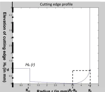
Representative function of cutting edge profile
In order to calculate the chips section, it’s necessary to define the cutting edge profile. The function Hk(r) is established, to give the elevation of each cutting edge point versus radius r. The lowest tool point « k » is defined at the elevation Z = 0. This function is decomposed into several successive functions, to take into consideration the different tool geometries.
Examples, the evolution of the function Hk(r) for a tooth without center cut, is represented Figure 5.
• If 0 < 𝑟𝑟 < 𝑅𝑅𝑐𝑐𝑐𝑐 :
𝐻𝐻𝑘𝑘(𝑟𝑟) = 𝑑𝑑
d is a value arbitrarily set to ensure the non-participation of the area during the machining.
• If 𝑅𝑅𝑐𝑐𝑐𝑐< 𝑟𝑟 < 𝑅𝑅𝑡𝑡− 𝑅𝑅𝑏𝑏 : 𝐻𝐻𝑘𝑘(𝑟𝑟) = [𝑟𝑟 − (𝑅𝑅𝑡𝑡− 𝑅𝑅𝑏𝑏)]. 𝑡𝑡𝑡𝑡𝑠𝑠 �𝜋𝜋2 − 𝜅𝜅𝑟𝑟� • If 𝑅𝑅𝑡𝑡− 𝑅𝑅𝑏𝑏< 𝑟𝑟 < 𝑅𝑅𝑡𝑡 : 𝐻𝐻𝑘𝑘(𝑟𝑟) = 𝑅𝑅𝑏𝑏− �𝑅𝑅𝑏𝑏2− [𝑟𝑟 − (𝑅𝑅𝑡𝑡− 𝑅𝑅𝑏𝑏)]2
κ
rTooth profile
with center cut
Tooth profile
without center
cut
Figure 2 : Tool geometry
Figure 3 : Feed definition.
Tool helical trajectory φi X HL
Y
θi Yoi Xoi CLi YciFigure 4 References definition
Calculation of the machined chip section by a tooth Hypothesis:
As the cutting speed is largely higher than the tool feed speed, two simplifying hypothesis are made:
• The tooth trajectory is considered circular (cycloid neglected) [Segonds et al., 2006]
• The calculation of volume machined by the tool at the present moment is the result of a Boolean subtraction operation between the volume of the machined work piece at the previous moment and the volume envelope of the tool, the tool being positioned on its trajectory.
Therefore, to calculate the chip section machined by a tool tooth « i » at the present time (the tool identified by its tool center’s point CLi) two calculation steps are made:
First, each point 𝐴𝐴𝑖𝑖 belonging to the envelope surface of the tool « i » is detected in 𝑹𝑹𝒐𝒐𝒐𝒐 from its coordinates (𝑋𝑋𝐴𝐴𝑖𝑖, 𝑌𝑌𝐴𝐴𝑖𝑖, 𝑍𝑍𝐴𝐴𝑖𝑖) in function of 𝑟𝑟𝐴𝐴𝑖𝑖 et 𝜑𝜑𝑖𝑖 (𝑟𝑟𝐴𝐴𝑖𝑖𝜖𝜖[0, 𝑅𝑅𝑡𝑡], 𝜑𝜑𝑖𝑖𝜖𝜖[0,2𝜋𝜋]), and the function 𝐻𝐻𝑘𝑘 applied at the tool « i » : 𝑨𝑨𝒐𝒐� 𝑋𝑋𝐴𝐴𝑖𝑖�𝑟𝑟𝐴𝐴𝑖𝑖,ϕ𝑖𝑖� = 𝑟𝑟𝐴𝐴𝑖𝑖. 𝑐𝑐𝑐𝑐𝑐𝑐ϕ𝑖𝑖 𝑌𝑌𝐴𝐴𝑖𝑖�𝑟𝑟𝐴𝐴𝑖𝑖,ϕ𝑖𝑖� = 𝑟𝑟𝐴𝐴𝑖𝑖. 𝑐𝑐𝑠𝑠𝑠𝑠ϕ𝑖𝑖 𝑍𝑍𝐴𝐴𝑖𝑖�𝑟𝑟𝐴𝐴𝑖𝑖,ϕ𝑖𝑖� = 𝐻𝐻𝑖𝑖(𝑟𝑟𝐴𝐴𝑖𝑖)
The set of the points 𝐴𝐴𝑠𝑠 for a constant 𝜑𝜑𝑠𝑠, represent the tooth where the chip section is assessed on.
Then, to identify the surface location previously machined on each point 𝐴𝐴𝑠𝑠, all the locations of the tool that interve before the location « i » on a complete orbit revolution are considered. It will then be possible to estimate the height of the machined material at the point 𝐴𝐴𝑠𝑠
.
Each considered previous location is identified by its tool center point CLk.The difference of altitude following
𝒁𝒁
between two tool locations CLi and CLk is called 𝐻𝐻𝑘𝑘𝑖𝑖. Knowing that the tool describes a helical trajectory characterized by its pitch P (Figure 3), the height 𝐻𝐻𝑘𝑘𝑠𝑠 is defined according to the relative angular position of CLi and CLk on the trajectory characterized by 𝜃𝜃𝑘𝑘𝑖𝑖 (Figure 6):𝐻𝐻𝑘𝑘𝑖𝑖 (𝜃𝜃𝑘𝑘𝑖𝑖) = 𝑃𝑃 −𝑃𝑃 × 𝜃𝜃2 × 𝜋𝜋𝑘𝑘𝑖𝑖
Then, for each tool point 𝐴𝐴𝑠𝑠 considered, the set of the point s 𝐴𝐴𝑘𝑘 of which the coordinates in the locator 𝑹𝑹𝒐𝒐𝒐𝒐 are such that
(
𝑋𝑋𝐴𝐴𝑘𝑘 = 𝑋𝑋𝐴𝐴𝑠𝑠 , 𝑌𝑌𝐴𝐴𝑘𝑘 = 𝑌𝑌𝐴𝐴𝑠𝑠)
are identified. The coordinate 𝑍𝑍𝐴𝐴𝑘𝑘 of the point 𝐴𝐴𝑘𝑘 can be calculated through the function 𝐻𝐻𝑘𝑘 :𝑨𝑨𝒌𝒌�
𝑋𝑋𝐴𝐴𝑘𝑘�𝑟𝑟𝐴𝐴𝑖𝑖,ϕ𝑖𝑖� = 𝑋𝑋𝐴𝐴𝑖𝑖 𝑌𝑌𝐴𝐴𝑘𝑘�𝑟𝑟𝐴𝐴𝑖𝑖,ϕ𝑖𝑖� = 𝑌𝑌𝐴𝐴𝑖𝑖
𝑍𝑍𝐴𝐴𝑘𝑘(𝑟𝑟𝐴𝐴𝑘𝑘, 𝜃𝜃𝑘𝑘𝑖𝑖) = 𝐻𝐻𝑘𝑘(𝑟𝑟𝐴𝐴𝑘𝑘) + 𝐻𝐻𝑘𝑘𝑖𝑖(𝜃𝜃𝑘𝑘𝑖𝑖)
For this the radius 𝑟𝑟𝐴𝐴𝑘𝑘 has to be previously determined. From Figure 6, by considering the triangle(𝐶𝐶𝐶𝐶𝑘𝑘, 𝐴𝐴𝑘𝑘, 𝐻𝐻𝐶𝐶) :
𝑟𝑟𝐴𝐴𝑘𝑘�𝑟𝑟𝐴𝐴𝑖𝑖,ϕ𝑖𝑖, 𝜃𝜃𝑘𝑘𝑖𝑖�
= ��𝑟𝑟𝑘𝑘𝑖𝑖2+ 𝑅𝑅𝑜𝑜𝑜𝑜𝑜𝑜2− 2 × 𝑅𝑅𝑜𝑜𝑜𝑜𝑜𝑜× 𝑟𝑟𝑘𝑘𝑖𝑖× 𝑐𝑐𝑐𝑐𝑐𝑐(𝜃𝜃𝑘𝑘𝑖𝑖− 𝛼𝛼)� With: 𝛼𝛼�𝑟𝑟𝐴𝐴𝑖𝑖,ϕ𝑖𝑖� = 𝑐𝑐𝑐𝑐𝑐𝑐−1 �𝑟𝑟𝑘𝑘𝑘𝑘2+𝑅𝑅𝑜𝑜𝑜𝑜𝑜𝑜2−𝑟𝑟𝐴𝐴𝑘𝑘2
2×𝑟𝑟𝑘𝑘𝑘𝑘×𝑅𝑅𝑜𝑜𝑜𝑜𝑜𝑜 �
And by considering the triangle(𝐴𝐴𝑖𝑖, 𝐻𝐻𝐶𝐶, 𝐶𝐶𝐶𝐶𝑖𝑖) :
𝑟𝑟𝑘𝑘𝑖𝑖�𝑟𝑟𝐴𝐴𝑖𝑖,ϕ𝑖𝑖� = ��𝑟𝑟𝐴𝐴𝑖𝑖2+ 𝑅𝑅𝑜𝑜𝑜𝑜𝑜𝑜2− 2 × 𝑅𝑅𝑜𝑜𝑜𝑜𝑜𝑜× 𝑟𝑟𝐴𝐴𝑖𝑖× 𝑐𝑐𝑐𝑐𝑐𝑐(𝜋𝜋 − 𝜑𝜑𝑖𝑖)�
For each point 𝐴𝐴𝑠𝑠 considered, points 𝐴𝐴𝑘𝑘 for every tool location « k » of the previous orbit revolution are calculated. To determinate the location of the machined surface, the point 𝐴𝐴𝑘𝑘 with the weakest altitude is kept and called 𝑆𝑆𝑘𝑘. 𝑺𝑺𝒌𝒌 ⎩ ⎨ ⎧ 𝑋𝑋𝑆𝑆𝑘𝑘�𝑟𝑟𝐴𝐴𝑖𝑖, ϕ𝑖𝑖� = 𝑋𝑋𝐴𝐴𝑘𝑘 𝑌𝑌𝑆𝑆𝑘𝑘�𝑟𝑟𝐴𝐴𝑖𝑖, ϕ𝑖𝑖� = 𝑌𝑌𝐴𝐴𝑘𝑘 𝑍𝑍𝑆𝑆𝑘𝑘�𝑟𝑟𝐴𝐴𝑖𝑖, ϕ𝑖𝑖� = min0≤𝜃𝜃𝑘𝑘𝑘𝑘≤2𝜋𝜋(𝑍𝑍𝐴𝐴𝑘𝑘)
The chip section on a tooth is then obtained by plotting the set of points 𝐴𝐴𝑖𝑖 and the associated points 𝑆𝑆𝑘𝑘, for a fixed angle 𝜑𝜑𝑖𝑖 (representing a tooth of the tool) and for 𝑟𝑟𝐴𝐴𝑖𝑖𝜖𝜖[0, 𝑅𝑅𝑡𝑡] (Figure 7).
This section is then split into trapezoids of thickness ℎ𝑘𝑘 and width 𝑏𝑏𝑘𝑘.
The thickness ℎ𝑘𝑘 is the normal distance to the tool profile between the profile 𝐴𝐴𝑖𝑖 and the previously machined surface 𝑆𝑆𝑘𝑘, it represents the chip thickness.
The width 𝑏𝑏𝑘𝑘 is the distance between points 𝐴𝐴𝑖𝑖, it is set arbitrarily. Hk (r) E le v a tio n o f c u tt in g e d g e H k (in mm) Radius r (in mm)
Figure 5 : Representation of the cutting edge profile « k » without cutting tool center
φi Ai Ak X HL CLk θki Y θi Xoi CLi Xθk α
Figure 6 Locating a tool “k” relative to the tool “i”
Xci
Rcc Rt-Rb Rt
d
MM Science Journal | Special Issue | HSM 2014
If the decomposition is sufficiently thin (small width 𝑏𝑏𝑘𝑘 compared to the radius of the tool), each trapezoid can be approximated and simplified by a rectangle. The chip section 𝑆𝑆𝑐𝑐 can then be written:
Sc(𝜑𝜑𝑖𝑖) = � 𝑏𝑏𝑘𝑘�𝑟𝑟𝐴𝐴𝑖𝑖, ϕ𝑖𝑖�. ℎ𝑘𝑘�𝑟𝑟𝐴𝐴𝑖𝑖, ϕ𝑖𝑖� Rt
𝑟𝑟𝐴𝐴𝑘𝑘=0
Calculation of the cutting force
The chip section in each moment being determined, the forces applied on the tool during drilling can be modeled. In this article, only the modeling of the cutting force normal to the chip section is presented and discussed. This effort is the most important and is the main cause of tool bending.
The other two components can be modeled in the same way.
The modeling approach is semi-analytical [Merchant, 1945], which gives for the same tool/work piece couple:
𝐹𝐹𝑐𝑐𝑐𝑐𝑡𝑡= 𝐾𝐾𝑐𝑐× 𝑏𝑏 × ℎ
Where 𝐾𝐾𝑐𝑐 is a specific cutting coefficient that will remain constant for the first part of the study and will be identified with calibration tests.
This model is applied to each trapezoid of the chip section and then summed to obtain the total cutting force when the tooth is in position 𝜑𝜑𝑖𝑖.
𝑑𝑑𝐹𝐹𝑐𝑐 𝑧𝑧𝑖𝑖(𝑟𝑟𝐴𝐴𝑖𝑖, 𝜑𝜑𝑖𝑖) = 𝐾𝐾𝑐𝑐× 𝑏𝑏𝑘𝑘(𝑟𝑟𝐴𝐴𝑖𝑖, 𝜑𝜑𝑖𝑖) × ℎ𝑘𝑘(𝑟𝑟𝐴𝐴𝑖𝑖, 𝜑𝜑𝑖𝑖)
𝐹𝐹𝑐𝑐 𝑧𝑧𝑖𝑖(𝜑𝜑𝑖𝑖) = � 𝑑𝑑𝐹𝐹𝑐𝑐(𝑟𝑟𝐴𝐴𝑖𝑖, 𝜑𝜑𝑖𝑖)
𝑅𝑅𝑡𝑡
𝑟𝑟𝐴𝐴𝑘𝑘=0
The evolution of the cutting force of a tooth on a tool revolution is calculated by varying 𝜑𝜑𝑖𝑖 from 0 to 2π (Figure 9).
This cutting force Fc zi(𝜑𝜑𝑖𝑖) must be calculated for each tooth of the tool, taking into account the differences in the tooth profile which may exist (ex: with or without center cut).
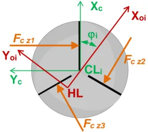
To calculate the resulting force, every effort is expressed in the orbital reference 𝑅𝑅𝑜𝑜𝑖𝑖, so (Figure 10):
𝑭𝑭𝒄𝒄 𝒛𝒛𝒛𝒛� 𝐹𝐹𝑐𝑐𝑐𝑐𝑡𝑡 𝑧𝑧1(𝜑𝜑𝑖𝑖). sin ( 𝜑𝜑𝑖𝑖) −𝐹𝐹𝑐𝑐𝑐𝑐𝑡𝑡 𝑧𝑧2(𝜑𝜑𝑖𝑖). cos ( 𝜑𝜑𝑖𝑖). 0 � 𝑅𝑅𝑜𝑜𝑘𝑘 𝑭𝑭𝒄𝒄 𝒛𝒛𝒛𝒛 ⎩ ⎨ ⎧ 𝐹𝐹𝑐𝑐𝑐𝑐𝑡𝑡 𝑧𝑧2�𝜑𝜑𝑖𝑖+ 2𝜋𝜋𝑍𝑍 � . sin ( 𝜑𝜑𝑖𝑖+ 2𝜋𝜋𝑍𝑍 ) −𝐹𝐹𝑐𝑐𝑐𝑐𝑡𝑡 𝑧𝑧2�𝜑𝜑𝑖𝑖+ 2𝜋𝜋𝑍𝑍 � . cos ( 𝜑𝜑𝑖𝑖+ 2𝜋𝜋𝑍𝑍 ) 0 ⎭⎬ ⎫ 𝑅𝑅𝑜𝑜𝑘𝑘 𝑭𝑭𝒄𝒄 𝒛𝒛𝒛𝒛 ⎩ ⎨ ⎧ 𝐹𝐹𝑐𝑐𝑐𝑐𝑡𝑡 𝑧𝑧3�𝜑𝜑𝑖𝑖+ 4𝜋𝜋𝑍𝑍 � . sin ( 𝜑𝜑𝑖𝑖+ 4𝜋𝜋𝑍𝑍 ) −𝐹𝐹𝑐𝑐𝑐𝑐𝑡𝑡 𝑧𝑧3�𝜑𝜑𝑖𝑖+ 4𝜋𝜋𝑍𝑍 � . cos ( 𝜑𝜑𝑖𝑖+ 4𝜋𝜋𝑍𝑍 ) 0 ⎭⎬ ⎫ 𝑅𝑅𝑜𝑜𝑘𝑘
The resulting force 𝑭𝑭𝒄𝒄 is then:
𝑭𝑭𝒄𝒄= 𝑭𝑭𝒄𝒄 𝒛𝒛𝒛𝒛+ 𝑭𝑭𝒄𝒄 𝒛𝒛𝒛𝒛+ 𝑭𝑭𝒄𝒄 𝒛𝒛𝒛𝒛
3 EXPERIMENTAL PROCEDURES
All tests were performed in a test piece in TiAl6V4 of 19mm thick. The cutting conditions are as follows:
Vc= 30mm/min; Fza=0.005mm/tooth; Sk Machined surface profile Ai Cutting edge profile E lev a ti on z ( in m m ) Radius rAi (in mm) hk Minimum distance
Figure 7 : Decomposition of the chip section
b
kdFc : Normal force in chip section
dFr : Radial force to the tool
dF
rdF
adF
cFigure 8 : Forces applied on the tool for a chip section
0
Tool revolution represented by ϕi2
π
M od ele d cu tt in g f or ce F c
Figure 9 : Evolution of the cutting force for a tooth without the center cut on a tool revolution
F
c z1
F
c z2
F
c z3
X
oi
Y
oi
X
c
Y
c
ϕ
i
CL
i
HL
Figure 10 : Representation of cutting forces on a tool with three teeth and with a single tooth with center cut.
Fzt= 0.04mm/tooth.
The tool used is a tool with three teeth (Z=3) ,with a single tooth with center cut and of diameter Dt = 9mm.
3.1 Identification of specific cutting coefficient To identify the specific cutting coefficient Kc, tests of slot machining were carried out on a machining center. The force measurement is performed using a Kistler dynamometer. The cutting coefficient, assumed to be constant, can be identified from the measurement of the maximum cutting force. The chip thickness is 0.04mm per tooth, the depth of cut is 0.75mm, and so the maximum chip section is 0.03mm ².
It can be deduced: 𝐾𝐾𝑐𝑐 =𝐹𝐹𝑐𝑐𝑚𝑚𝑚𝑚𝑚𝑚 𝑆𝑆𝑐𝑐𝑚𝑚𝑚𝑚𝑚𝑚
Maximum force Fxy observed during the test is 105N. This gives a specific cutting coefficient for our tool/work piece couple of: Kc = 3500N/mm ².
This Kc value is a first approximation for model validation. It doesn't take into account influence of chip thickness or possible influence of speeds. And thereafter, two coefficient will be identified, one for the axial part and one for radial part, because the radial and axial parts present different cutting angles.
3.2 Force measurement in orbital drilling
Tests are also conducted in orbital drilling, in order to have a database to validate the modeling. These tests are performed on a drill bench equipped with an orbital spindle. On all tests, cutting forces are recorded using the dynamometer Kistler and sampled at 10 kHz. On the signals obtained when measuring just a taring is performed.
The hole diameter is 11.1mm and it is made with the same tool which has diameter of 9mm.
Three different geometry tools are tested (Figure 11). Only the axial part is different. The first tool is the tool previously studied with one teeth with cutting tool center and the tool cutting edge angle κr=93°. The second tool is a similar tool, only the tool cutting edge angle is different. The axial part of the second tool is flat so κr=90°. The third is the same than the second without the cutting tool center.
Figure 11 : The different geometry tool
For comparison of the three tools, cutting conditions have remained the same and are the conditions recommended by the manufacturer: Vc=30m/min; fa=0.013mm/rev; ft=0.12mm/rev.
4 RESULTS AND DISCUSSIONS
The Kistler 9257B dynamometer allows measuring the resultant force in the plane normal to the axis of the tool Fxy
With 𝐹𝐹𝐹𝐹𝐹𝐹 = �𝐹𝐹𝐹𝐹2+ 𝐹𝐹𝐹𝐹2 (Figure 11)
The force FcT obtained by modeling differs from the real effort measured Fxy (Figure 11)
The evolution of the modeled force on a tool revolution shows the successive passage of three teeth. This is explained by the fact that the radial chip is not constant on the tool revolution. In addition there is a single tooth with center cut, therefore causing disruption on the tool revolution.
The force measurement Fxy shows only two peaks of effort. Either the force is compensated perfectly on the third revolution, or either the chip is not constant for all three teeth.
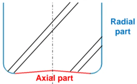
This difference between the two graphs is the lack of taking into consideration of cutting phenomena. To improve the model, the tool will be divided into two different parts, in order to better understand how each part works. The axial and radial parts of the tool is defined as (Figure 12).
The tool performance and the cutting phenomena caused by the radial part of the tool are known and already considerably studied in the literature. Modeling the cutting force of the axial part is more complex because the tool profile of the tip (Figure 12) combined with the tool trajectory is not classical.
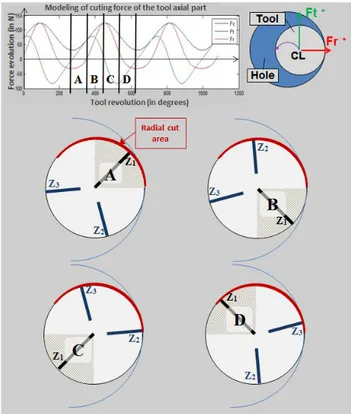
In order to better understand the mechanisms during drilling, the evolution of the tangential force Ft at the contact point tool / work piece (according to Yoi) and of the radial force Fr (Figure 14) are modeled.
These two efforts strongly oscillate on a tool revolution, causing a variable bending force of the latter.
So a dynamic phenomenon is established and must be taken into account in the model to adjust the chip thickness of the radial cut. The Figure 14 shows that when the tooth with center cut is located in the "A" area (0 < 𝜑𝜑 < 𝜋𝜋
2), the radial force and tangential force are positive but quite low, not causing a significant modification in radial section.
When the tooth with center cut (z1) is located in the "B" area (3𝜋𝜋
2 < 𝜑𝜑 < 2𝜋𝜋), the radial force and tangential force
N°1:
│ N°2:
│ N°3:
κr=93°│
κr=90°│
κr=90°with cutting tool center
│
withoutTool revolution (in degrees)
One tool revolution
for ce e volu tion F c
Figure 12: Comparison of the evolution of the cutting force over three revolution of tools (modeling at top; measure
down for the tool n°1)
Radial part
Axial part
MM Science Journal | Special Issue | HSM 2014
are positive. Therefore this resultant force tends to push the tooth being machined towards the surface.
When the tooth with center cut is located in the area "C", the radial force is positive and tangential force is negative. Therefore this resultant force tends to push the tooth (z2) towards hole surface and in reverse tends to withdraw the tooth (z3) of hole surface.
And when the tooth with center cut is located in the area "D", the radial and tangential force are negatives. Therefore this resultant force tends to withdraw the tooth (z3) of hole
Figure 14 Modeling of the radial and tangential force of the tool axial part, taking into account the three teeth. The hypothesis is that the radial section isn't homogeneous for the three teeth, because bending forces are different to each passage of various teeth on the radial cut area. The radial chip thickness machined by the tooth z2 is greater than that machined by the tooth z3.
In order to bring out this dynamic phenomenon, a series of holes is created with each tool, with the similar conditions (material, cutting parameters, hole diameter) for each tool. And then the diameters of the holes will be measured on the three-dimensional measuring machine (MMT).
Figure 15 : Average profile measured on the hole for each tool
These measurements show that with same cutting conditions the profile of the hole can be different. And especially that the axial part of the tool is very important on the profile, therefore on the bending tool.
On the profile of the first tool the entrance hole diameter is larger than output. This validates the result of the modeling of the cut (Figure 14) that the cut of the axial part
of the tool causes a positive average radial force, increasing the hole diameter. And at the end of the drilling there is no cutting of the axial part therefore the diameter of the hole decreases.
Between the profile of the first tool and the second, only the tool cutting edge angle is different. The influence of this angle on the axial chip is showed on the Figure 16.
Figure 16 : influence of tool cutting edge angle on the axial chip geometry
Therefore the axial chip for the second tool is more homogeneous, which can be seen also on the modeling effort. The maximum radial force modeled for the second tool is 100N whereas for the first tool it's 150N, it's a reason why the variation of hole diameter is less important for the second tool
Figure 17 : Modeling of the cutting force of the tool axial part for the three tools
As regards the third tool, the three teeth are identical and the axial part is flat so the chip is identical for the three teeth. That is why the model shows no cutting force because the forces on each tooth cancel each other. Without the radial force generated by the axial part, the tool during the drilling bend and therefore realized a smaller diameter. The increase of diameter at the end of drilling, is due to the relaxation of the tool.
5 CONCLUSIONS AND PERSPECTIVES
This model, with the integration of the tool geometry, allowed knowing the exact geometry of the chip. With this knowledge, the modeling of the cutting force is possible which allows a better understanding of the cut phenomena when orbital drilling with a specific tool. It is therefore possible to vary the tool geometry or the cutting conditions in the model to predict the cutting forces, and thus be able to optimize these parameters. If the link between effort and drilling defects are known (ex: bending force → decrease in diameter), it is possible to optimize these parameters to improve the quality of the hole
However, further work is needed to improve the model. As integrate in this model coefficients which evolve in function of the chip thicknesses. And especially which integrates the drilling dynamic, so that the model and the measurements are identical.
6 ACKNOWLEDGEMENTS
This work was carried out within the context of the working group Manufacturing'21 which gathers 18 French research laboratories. We would also like to thank the project called OPOSAP (Optimisiation du Perçage orbital avec Surveillance Active du Process) and above all the partners who helped us to make this research.
7 REFERENCES
[Brinksmeier et al., 2008] Brinksmeier, B; Sascha Fangmann.; Meyer, I; "Helical milling of CFRP-Titanium layer compounds"; In: Prod. Eng. Res. Devel , pp. 2:277– 283; Germany 2008
[Denkena et al., 2008] Denkena, B; Boehnke, D; Dege, J.H.; "Helical milling of CFRP-Titanium layer compounds"; In: CIRP Journal of Manufacturing Science and Technology, pp. 64-69; Germany 2008
[Fontaine, 2004] Fontaine, M ; "Modélisation thermomécanique du fraisage de forme et validation expérimentale" Thesis at Metz University ; France ; 2004 [Lorong et al., 2008] Lorong, P; Ali,; "Logiciel explicite en thermomécanique pour la simulation et la formation d’un copeau en usinage"; In: Mécanique et industrie, pp. 343-349; Vol3 ; 2002
[Lutze, 2008] S. Lutze. State of the art and expectations for the future of orbital drilling. Thesis at Leuphana University Lüneburg School III 2008
[Merchant, 1945] M.E.Merchant. Mechanics of the metal cutting process, I.Orthogonal cutting, In :Journal of Applied physics, vol 16 p318-324 . 1945
[Oxley, 1989] Oxley, P.L.B. Mechanics of metal cutting, Ellis horwood, Chichester, UK, 1989
[Segonds et al, 2006] S.Segonds, Y.Landon, F.Monies, P.Lagarrigue, Method for rapid characterisation of cutting forces in end milling considering runout, in: International Journal of Machining and Machinability of Materials, vol. 1 (1), pp. 45-61, 2006.