Scheduling real-time systems with cyclic dependence using data criticality

Titre:

Title

:

Scheduling real-time systems with cyclic dependence using data

criticality

Auteurs:

Authors

:

Imane Hafnaoui, Rabeh Ayari, Gabriela Nicolescu et Giovanni

Beltrame

Date: 2017

Type:

Référence:

Citation

:

Hafnaoui, I., Ayari, R., Nicolescu, G. & Beltrame, G. (2017). Scheduling real-time systems with cyclic dependence using data criticality. Design Automation for Embedded Systems, 21(2), p. 117-136. doi:10.1007/s10617-017-9185-9

Document en libre accès dans PolyPublie

Open Access document in PolyPublie

URL de PolyPublie:

PolyPublie URL: http://publications.polymtl.ca/2546/

Version: Version finale avant publication / Accepted version_{Révisé par les pairs / Refereed} Conditions d’utilisation:

Terms of Use: Tous droits réservés / All rights reserved

Document publié chez l’éditeur officiel

Document issued by the official publisher

Titre de la revue:

Journal Title: Design Automation for Embedded Systems

Maison d’édition:

Publisher: Springer

URL officiel:

Official URL: https://doi.org/10.1007/s10617-017-9185-9

Mention légale:

Legal notice: The final publication is available at Springer via9185-9 https://doi.org/10.1007/s10617-017-Ce fichier a été téléchargé à partir de PolyPublie,

le dépôt institutionnel de Polytechnique Montréal This file has been downloaded from PolyPublie, the

institutional repository of Polytechnique Montréal http://publications.polymtl.ca

(will be inserted by the editor)

Scheduling Real-Time Systems with Cyclic

Dependence Using Data Criticality

Imane Hafnaoui · Rabeh Ayari · Gabriela Nicolescu · Giovanni Beltrame

Received: XX.XX.XXXX / Accepted: XX.XX.XXXX

Abstract The increase of interdependent components in avionic and automotive software rises new challenges for real-time system integration. For instance, most scheduling and mapping techniques proposed in the literature rely on the avail-ability of the system’s DAG representation. However, at the initial stage of system design, a dataflow graph (DFG) is generally used to represent the dependence between software components. Due to limited software knowledge, legacy compo-nents might not have fully-specified dependencies, leading to cycles in the DFG and making it difficult to determine the overall scheduling of the system as well as restrict access to DAG-based techniques. In this paper, we propose an approach that breaks cycles based on the assignment of a degree of importance and that with no inherent knowledge of the functional or temporal behaviour of the compo-nents. We define a “criticality” metric that quantifies the effect of removing edges on the system by tracking the propagation of error in the graph. The approach was reported to produce systems (56 ± 14)% less critical than other methods. It was also validated on two case studies; a data modem and an industrial full-mission simulator, while ensuring the correctness of the system is maintained.

Keywords Execution order assignment · Real-time systems · System scheduling · System integration · Data criticality · Cyclic dependency · Directed acyclic graph

1 Introduction

When scheduling complex real-time systems, such as those encountered in the avionic and automotive industries, engineers widely rely on a representation of the system in the form of a directed acyclic graph (DAG). This is usually referred to as a task graph in which nodes represent system components and edges, the communication between them. A system component is an encapsulated entity treated as a simple task and mapped and scheduled in the same manner. A DAG

Imane Hafnaoui

2900, Boulevard ´Edouard-Monpetit, Montr´eal, QC, Canada, H3T 1J4. E-mail: imane.hafnaoui@polymtl.ca

representation of a system is the basic input for various methodologies proposed in literature. The motivation of these works vary from the analysis of system performance and feasibility [3] to the optimization of the mapping and scheduling of real-time systems [1, 4], to involving artificial intelligence to solve the issue of real-time scheduling [17]. Some tools such as YARTISS [5] and STORM [31] use a DAG as an input model to simulate the real-time behaviour of the system. In large-scale system development, it is generally assumed that the DAG representation is available at integration time. However, the reality on the industrial level says otherwise. Legacy components and architectures are oftentimes not fully specified which limits the availability of a DAG. Instead, the system representation is limited to a generic model such as the one in Figure 1a.

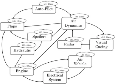
A generic avionic subsystem is shown in Figure 1a with the edges representing the flow of data between the components and the bubble stating the id. and rate at which they are executed. These are among other characteristics specific to every component that we formally define in Section 3. Scheduling this system becomes tedious even under a simple application of Rate Monotonic scheduling (RMS) with dependent tasks. However, with the DAG representation of the system in Figure 1b, in which the cycles are removed, one possible schedule for the system under a pre-emptive RMS can be achieved as in Figure 1c and further methods to optimize certain objective metrics such as the throughput or the energy of the system become possible; an option that was very limited with the graph of Figure 1a.

The inability to identify the execution order of the system components at integration time is a consequence of many scenarios, one of which is expecting engineers from different domains, such as mechanics, electrical engineering, etc., to be experts in their fields as well as software engineering. Moreover, due to the complexity of these systems, code is repeatedly reused to decrease time-to-market and cost of software testing. On top of this, the system design sometimes requires the use of an Original Equipment Manufacturer (OEM)’s product which generally comes in the form of a binary component accompanied with a file to describe the component’s inputs and outputs, often without specifying the inter-dependence nor the latency of a component. In all of these cases, the system components are viewed as black boxes which makes it difficult to gather concrete information about the components, unless specified by the designer. This limits the integration experts’ accessibility to the system’s task graph.

To model such systems, a dataflow graph (DFG) is employed to represent the dependence between components as well as the amount of data exchanged. However, different components are interconnected in such a way that their com-putations depend on the data generated by other components. This naturally creates cycles within the graph which complicates the scheduling process, as well as precedence assignments that schedulers will have to take into consideration. Furthermore, the existence of cycles in the system puts a hindrance to the appli-cation of many analysis tools and optimization techniques that are available for acyclic directed graphs.

Generally, integration engineers rely on the feedback of legacy component de-velopers and their own expertise and knowledge of the components individual functionality acquired through the years to split the cycles. Alongside integration problems, this creates issues in other disciplines such as co-simulation. For the purpose of system verification and validation, different components are simulated

Spoilers id5, 10ms Auto-Pilot id1, 10ms Engine id4, 20ms Air Dynamics id3, 10ms Visual Cueing id10, 10ms Air Vehicle id6, 50ms Electrical System Id7, 40ms Hydraulic id8, 40ms Flaps id2, 10ms Radar id9, 10ms

(a) DFG representation of the system with cyclic dependences.

Spoilers id5, 10ms Auto-Pilot id1, 10ms Engine id4, 20ms Air Dynamics id3, 10ms Visual Cueing id10, 10ms Air Vehicle id6, 50ms Electrical System Id7, 40ms Hydraulic id8, 40ms Flaps id2, 10ms Radar id9, 10ms

(b) DAG representation of the system after cycle breaking.

AirDynamics Auto-Pilot Spoilers Flaps Radar Visual Q. Engine Electrical Hydraulic Air Vehicle 10 20 30

(c) System scheduled under a pre-emptive RMS.

using varied technologies. If we look at a simulation of an avionic system as an example, the tools used to simulate the electrical system are different from those that simulate the aerodynamics. In some cases, parts of the system are physi-cally available, however presented as black boxes and engineers are required to co-simulate the rest of the system with limited knowledge about the components. The presence of cycles in the overall mapping of the system drives engineers to rely on recursive techniques to reach sound simulation results. Having a good initial configuration to the recursive process could reduce the design time extensively.

One popular approach to model systems that involve cyclic dependences is Synchronous dataflow graphs (SDFs). The authors of [30] presented a modular approach to analyze system performance that was applied directly to a cyclic SDF. The scheduling of an SDF was optimized in [6] using evolutionary techniques by considering the limitation of the size of the scratchpad memory. Although these approaches yielded good results, this model decreases the scope of approaches that study real-time systems since it excludes approaches based on DAGs. To this endeavor, other works [27, 29, 32] have been proposed to unfold an SDF into a DAG by simply discarding the edges that contained delays. This makes DAG-based approaches to analyze and optimize the system accessible. For all that, these methodologies cannot be adapted to the problem that we presented so far for the sole reason that the edge property, delay, encountered in SDFs is among the metadata that are not available at integration time as discussed in the previous scenarios.

In this paper, we put forth an approach to transform a DFG with cyclic data dependencies into a DAG, with no inherent knowledge of the function and be-haviour of system components for the purpose of opening access to DAG-based techniques. In here, we focus on simulations of real-time systems and systems such the informatics in automotive systems which are comprised of components with soft deadlines and scheduled under static schedulers. This is the case since certain standards are enforced when scheduling these types of real-time systems. Especially with the prevalence of the Integrated Modular Avionics (IMA) [20] to design avionic systems, static scheduling policies are preferred and sometimes imposed to enforce predictability in the system.

The approach we propose here is based on the idea of error propagation to elim-inate cycles. We introduce a concept that describes the importance of data, which we label criticality, in which the effect of removing a certain edge is quantified as a characteristic of the data being carried by the edge. This is a key component in deciding which edges to discard and transform the DFG into a DAG.

The rest of the paper is structured as follows: Section 2 summarizes the work that has been proposed in literature to solve this issue; Section 3 gives a description of the system model. The approach to eliminate cycles based on criticality is detailed in Section 4 followed by a motivational example; The results obtained from a set of experiments and two case studies are reported in Section 5; Finally, conclusions are given in Section 7.

2 Related work

One of the important parameters that characterizes tasks in real-time system scheduling is their priority assignment. This, alongside task precedence constraints,

could decide the schedule that drives the execution of the system. The assignment is generally attributed with a performance objective in mind decided by the de-signer when building the system such as schedule length, schedulability, etc.

Different approaches have been proposed to schedule the system and assign priorities with task dependences in mind. The authors in [25] and [21] tackled the issue from a mapping point of view in which a Genetic Algorithm (GA) was employed to allocate dependent tasks and assign priorities on a multiprocessor system. The Distributed by Optimal Priority Assignment (DOPA) heuristic was proposed in [9] to address both the problem of finding a partitioning configuration and a priority assignment for tasks on a core that ensures the tasks don’t miss their deadlines. The problem is extended to Network-On-Chip (NoC) systems in the work of Liu et al. [18] who proposed a dependency-graph based priority as-signment algorithm (eGHSA) targeting NoCs with shared virtual-channels. On the other hand, the works in [7, 14, 19] relied on the system topology and focused on the basic idea that priorities should be chosen by the node’s relative importance. In [15, 16], the concept of Global Critical Path is introduced which extends the top-level and bottom-level strategies by considering the critical path in the graph (the longest path from the source to the exiting node) and its branch paths. Sin-nen et al. [26] proposed multiple extensions of the previous schemes to include communication contention and the number of successors. Be that as it may, the constant assumption seems to be that a graph representation of the system as a directed acyclic graph (DAG) is available. Other models that include cyclic de-pendences were proposed to bypass the issue of DAG inaccessibility. The work in [11] extended TTIG (Temporal Task Interaction Graph) [22]; a different model from a DAG that models cycles and bypasses some of the drawbacks of using a DAG. However, the cycles within this model were viewed as special nodes re-ferred to as Composite Nodes to facilitate computation of path execution times and the presence of cycles was not dealt with head-on. A similar approach was proposed by Sardinha et al. [24] in which cycles were included in a special group called Strongly Connected Components (SCC) to facilitate mapping of tasks onto a number of processing elements. The authors in [23] proposed a modified Depth First Search (DFS) algorithm that splits the cycles. Yet, once again, the assump-tion was that all edges are of the same importance and the focus of the paper was on shortening the critical path of the resulting DAG to reach a better makespan for scheduling the DAG. The presence of cycles in attack graphs in the field of cyber security was addressed by Huang et al. [12] in which the authors identify two types of cycles; the ones that cannot be executed irrespectively of which edge was removed and hence discarded the cycle, and those that cannot be removed. The approach relies on the functionality of the nodes and characteristics specific to security modules to remove the cycles and hence cannot be generalized to other scenarios from different domains.

In this work, we set forth a methodology to break the cycles in a dataflow graph with no inherent knowledge of the components behaviour or execution times that relies on a definition of data criticality.

3 System Model

In this paper, we deal with systems similar to full-mission simulators (FMS) in which system components are viewed as tasks with execution times, deadlines and execution rates, and thereby mapped and scheduled as a generic taskset. To be able to visualize the system, better understand the dependencies and build our ap-proaches on mathematical grounds, we define two types of graphs; the dependence graph and task graph.

Due to the partially specified components, the dependence graph represents the system at its raw state. The exchange of data between components is used to track the intra-component communication and build the dependence graph. Note that the components that depend on the data produced by other components do not wait for said data to be generated to start executing. Rather the data is accessed through a shared memory. This, in turn, implies that, depending on the schedule, the data read by a component at a point in time could be possibly out-dated. This is another reason synchronous dataflow graph are not suitable to model our system since the nodes or actors in a SDF wait on certain tokens to start executing. For such, we choose to rely on a generic DFG to model the dependence graph.

On these grounds, we model our system’s dependence graph with a dataflow graph G = (V, E) where the nodes V = {t1, t2, ..., tn} represent the components

that make up the system and E = {e11, e12, ..., ekp}, the set of edges eijthat link

components ti and tj. It is worth noting that self-loops, defined as data generated

by a component and read by the same component, are ignored since they have no effect on the execution order of the components.

The common representation of systems found in literature is that of a task graph, onto which we aim to transform the above defined DFG. A task graph is a directed acyclic graph, ˜G = ( ˜V , ˜E), in which the nodes ˜V = {τ1, τ2, ..., τn}

represent a job instance of the component V . A job τi is characterized as a tuple

{Idi, Ci, di, Ti} defined as the identifier, execution time, absolute deadline, and

period respectively. The edges ˜E represent the precedence between the jobs and describes the constraint on the execution order of the jobs.

As can be seen from Figure 1a, component communication does not imply iden-tical periodicity. In other words, two components communicating with each other does not necessarily translate to them executing at the same rate. This charac-teristic is important to identify especially when certain schedulers are considered. With scheduler policies that rely on task deadlines and periods to assign priorities, multiple components are assigned the same priority in execution and the number of tasks with the same priority becomes large as the system grows in size. If we take as an example a taskset with three tasks (t1, t2, t3) with periods {16, 32, 16}

respectively, and we schedule them under a Rate Monotonic scheduler, the RMS algorithm will assign priorities P = 2 for task t2 and P = 1 for both tasks t1

and t3. The need to assign execution orders for tasks with similar priorities

be-comes necessary when scheduling a dependent set of tasks in which precedence is a constraint.

Furthermore, we argue that analyzing the overall system to break all cycles is unnecessarily time-consuming since data produced by components with shorter periods can be consumed at a later time by the components with larger periods. Component Spoilers in Figure 1a for example might produce data every 10 (ms). However, Hydraulic only consumes the data once every 40 (ms) making it

irrel-B

C

A

A

C

B

C

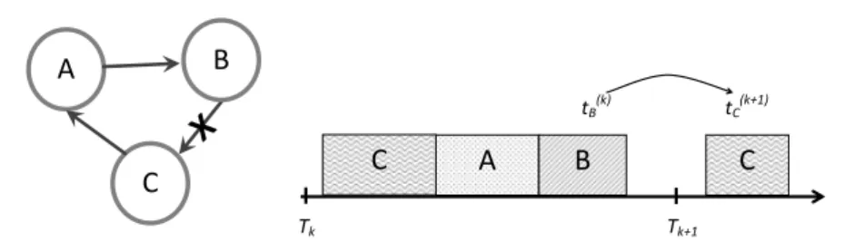
Fig. 2: The effect of splitting a cycle in a real-time system.

evant whether Hydraulic is consuming the data generated in the first period of Spoilers or the last.

4 Graph Transformation Through Data Criticality

The graph transformation refers to breaking the cycles present within the depen-dence graph to be able to schedule the resulting task graph. In the context of scheduling soft real-time systems, cycle breaking involves the decision of which components can tolerate delay. Our approach relies on the definition of a new pa-rameter that characterizes the data exchanged between the components that we label data criticality.

4.1 Error Propagation Approach (EPA)

Data criticality comes from the understanding that some data generated by some components are more important than other data. In here, the importance of data expresses how affected the system would be if the data were erroneously computed. Since our problem is a scheduling issue, in which the system components are scheduled in a certain order within one time period, breaking cycles by removing edges in the graph does not involve loss of data but rather results in one of the data generated to be “out-dated”. This is to say that when edge eijis removed, the

kthjob τ_j(k)of the component at the tail tj will use data generated by component

ti in the previous time period, τi(k−1), to complete its inner computations. This

can be observed in the example shown in Figure 2.

Since the system components are viewed as black boxes and the knowledge of the interactions of input and output variables within a component is unavailable, it is difficult to determine which components can tolerate out-of-date data. For such, we label the data generated by a component that is using outdated information as “faulty data”. By modelling this behaviour as an error injection mechanism, we propose a method that computes the criticality of the data based on the prop-agation of the error within the system graph and that with no knowledge of the components’ functionality. This involves four steps:

1. Extraction of all graph cycles;

2. Calculation of the rate of error propagation within the system graph from every component in the cycles;

4. Removal of appropriate edges to break the cycles.

In the following, we detail every step and provide insight into their implemen-tations.

4.1.1 Cycle Extraction

A simple cycle is defined as a path Γc= {t1, t2, ..., tk} in which the head node is

the same as the tail node with no repetitive nodes or edges, except for the head and tail nodes. We implemented an algorithm based on the work presented in [13] to extract the cycles present in the graph G. The time complexity of this algorithm is reported as O((n + e)(c + 1)) for a graph with n nodes, e number of edges and c number of simple cycles.

4.1.2 Error Propagation

By adopting the definition that removing an edge translates to a component using old data and hence generating faulty data, the algorithm follows the propagation of this erroneous data within the graph. Although we can easily follow the dependence between components given a dependence graph, there is no definitive way to track the dependence of a component’s outputs to its input variables unless provided by the designer.

To avoid making assumptions about the components, an element of stochas-ticity is introduced. The behaviour of the erroneous data when consumed by a component can have two behaviours within a component.

– State A in which the error disappears if the faulty data gets overwritten by the component’s inner calculations. A simple example of this is the case in which the faulty variable x is initialized if certain conditions are fulfilled.

[ . . ] if ( C o n d i t i o n s == T r u e ) do : x = x_0 end if z = x - 10 [ . . ]

– State B in which the error propagates to other output variables that include the faulty variable x in their computations as a function f (x), which allows the error to propagate from the component to the components of the system that directly depend on it.

[ . . ] y = x ^2 + z if ( C o n d i t i o n s == T r u e ) do : x = x_0 end if [ . . ]

We define Ai as the event of component ti producing an error in which:

Ai=

(

1, if the error is propagated.

0, if the error is masked. (4.1)

The problem can be viewed as a set of Bernoulli trials in which every component has the probability of internally propagating an error defined as:

P r(Ai) =

(

pi, if Ai = 1.

qi, if Ai = 0.

(4.2)

where pi represents the probability of a component propagating an error from

its inputs to its outputs, and qi = 1 − pi, the probability of masking the error.

This is not to be confused with the probability of a component generating or containing a software bug since the components are assumed to be bug-free at integration time.

We define P red(ti) and Succ(ti) as the list of predecessor and successor

com-ponents of ti respectively. Assuming that P red(ti) = {tj}, the observation of an

error at the output of ti depends on tj

P r(Ai= 1|Aj= 1) = pi,

P r(Ai= 1|Aj= 0) = 0

We want to find the probability of a component propagating an error to its successor dependants with the probability of the error having propagated from its predecessor components. In other words, it is the probability of events Ai and Aj

having occurred, where tj ∈ P red(ti) and tj ∈ Succ(t/ i).

The unconditional probability of ti propagating an error is

P r(Ai= 1) = P r(Ai= 1, Aj = 1) + P r(Ai= 1, Aj = 0)

= P r(Ai= 1|Aj= 1)P r(Aj= 1) + P r(Ai= 1|Aj = 0)P r(Aj= 0)

= P r(Ai= 1|Aj= 1)P r(Aj= 1)

= piP r(Aj = 1)

(4.3)

Events Aj are independent, however, they are not mutually exclusive since

components tj can contain and propagate an error at the same time. For more

than one predecessor component, Equation 4.3 can be generalized as

P r(Ai = 1) = P r(Ai = 1, (∪tj∈P red(ti)Aj= 1)) (4.4)

In the case that ti has no predecessors, we are dealing with the faulty

com-ponent at which we are injecting the error and the probability of propagation is P r(Ai = 1) = 1. A weighted graph Ω(tx) = (V, ω(tx)) is built by calculating the

probability of error propagation from the faulty component tx to all its directly

and indirectly connected components by assigning weights ωij(ti) to the edges

t

t

t

t

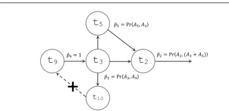
Fig. 3: Direct and Indirect Error Propagation results in weighted graph Ω(t9).

Step 1. Given a cycle Γ , an edge eli is selected to study the effect of its

removal on the system. The component at the tail of the edge is assumed to be the faulty component and the data it generates as erroneous. We calculate the direct error propagation by looking for the component directly connected to the faulty component and assign a weight ωij(ti) = 1 to the edges connecting

the faulty component ti to its successor components tj| tj∈ Succ(ti).

Step 2. Once the direct error propagation is assigned, we calculate the indi-rect error propagation by employing Equation 4.4 considering the components tk that depend on the faulty component through other intermediate

compo-nents and assign weights ωjk(ti) = P r(Aj = 1) to the edges connecting these

components to the intermediate components.

Step 3. We rely on a Breadth First Search (BFS) to look for lower level components that indirectly connect to the faulty component and repeat Step 2 until the last dependent component is reached and appropriate weights are assigned to the connecting edges. The result is a weighted graph Ω(ti) with the

probabilities of the error propagating from the designated faulty component ti.

Figure 3 represents part of the system of Figure 1a and gives a visual example of how Equation 4.4 is used when we track the propagation of error from component t9 to the rest of the subgraph. We can see that the directly dependent component

t3will have a probability of ˆp9= 1 to receive faulty data at its input. To calculate

the probability of indirect propagation of error from component t3 to [t2, t5, t10],

we use Equation 4.3 as

P r(At3 = 1) = P r(At3= 1|At9= 1)P r(At9 = 1)

= pt3P r(At9 = 1)

= pt3

The same is done for the probability of the error propagating from compo-nent t2. Considering that t2 depends on both t3 and t5, the probability of the

error propagation P r(At2 = 1) is the probability of event At2 occurring with the

probabilities of events At3 and At5 having occurred respectively in which case

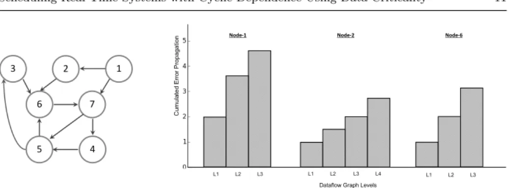
1 2 6 7 5 4 3 L1 L2 L3 L1 L2 L3 L1 L2 L3 L4 Cumula te d E rr or Pro pa ga tio

n Node-1 Node-2 Node-6

Dataflow Graph Levels

Fig. 4: Example: CEP for three different nodes

4.1.3 Cumulated Error Propagation

Once the error propagation probabilities of a faulty component are calculated, the result is a weighted graph Ω(ti) for every edge that belongs to a cycle as in the

example graph of Figure 3.

The amount of propagation of an error in the system determines the global effect of removing an edge on the system. To quantify this effect, a cumulated error propagation (CEP ), that expresses the criticality of data, is calculated as

CEP (tx) =

X

i,j∈Ω(tx)

ωij(tx) (4.5)

The example shown in Figure 4 illustrates how the error accumulates as it spreads in the system DFG when it transfers from one level to another for different faulty nodes of the same graph. A level is defined as a subset of components which have an equal number of hops (i.e. longest distance) to the root component; ti. For

the example given in figure 3, both components t5 and t10 are at level 2 whereas

component t2 is at level 3.

Figure 4 shows that the CEP is not affected by how deeply the error spreads through the graph, but rather by the outdegree centrality of the studied compo-nent. This is the case since the probability of an error propagating is higher at the first levels and becomes lower as we go deeper and further from the root faulty component since the faulty data have more chances to be overwritten. That is to say that the denser the levels directly connected to the faulty component, the higher the CEP is going to be.

Given this definition, the component within the cycle with the minimum CEP has the smallest effect on the system, which will decide the edge to be remove to break the cycle.

4.1.4 Minimum Feedback Arc Set with Criticality

Our proposed approach described so far is only concerned with breaking the cycles by removing the edges that carry the least critical data within a cycle. However, in most cases, an edge belongs to more than one cycle. Hence, removing an edge from a cycle might also break other cycles. This means that the number of edges that are to be removed is:

Algorithm 1: Error Propagation Approach (EPA): Cycle breaking algo-rithm based on data criticality.

Input: A dependence graph G = (V, E).

Output: A transformation of G to a task graph ˜G.

1 Load the dependence graph G;

2 Cycles = simple cycles in G;

3 for cycle in Cycles do

4 for edge in cycle do

5 Calculate probability of error propagation P r(Ai= 1) from component tx; 6 Assign probability to edge weights ωij(tx) ;

7 Build weighted graph Ω(tx) with error propagation probabilities; 8 Attribute the Cumulated Error Propagation CEP (tx) to edge;

9 end

10 Add edge with minimum(CEP) to Temporary Edges list;

11 end

12 Calculate “popularity” of edges in Temporary Edges;

13 Sort Temporary Edges according to popularity;

14 while Cycles do

15 Add P opular edge to the Removed Edges list Υ ;

16 Update Temporary Edges and Cycles lists ;

17 end

18 Remove edges ˜eij∈ Υ from ˜G.

X

eij∈Υ

eij≤ c (4.6)

where c is the number of simple cycles in the graph., and Υ the set of removed edges.

To optimize our approach, we address the problem as a Minimum Feedback Arc (MFA) set problem. This refers to a set of NP-Hard problems that take a non-polynomial time to find the minimum number of edges to remove in order to break all cycles.

Since our main concern is removing edges based on the criticality of data they carry, solving the MFA problem is out of the scope of this paper. Nonetheless, we want to base the decision of removing edges on data criticality while reducing the number of edges that could break all cycles. For this purpose, we introduce the concept of “popularity” among edges. We define the “popularity” of an edge eij

as the frequency of appearance f (eij) of an edge in the cycles Γc. Formally,

f (eij) = X eij∈Γ f c eij (4.7)

Accordingly, we extend the criticality based solution to lower the number of removed edges by first sorting the set of edges that EPA suggested to discard and then remove the most popular edges one by one until all cycles are broken (12−17). Algorithm 1 summarizes the methodology to break cycles within a dependence graph that relies on data criticality and consequently transforms the DFG into a DAG. The algorithm has a time complexity of O((n + e) · ce) for a graph with n components, e number of edges and ce number of total edges in c number of simple cycles.

t3

t5

t1

t2

t9 t10

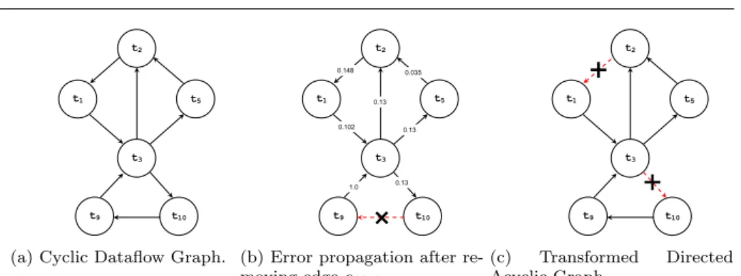
(a) Cyclic Dataflow Graph.

t3 t5 t1 t2 t9 t10 1.0 0.13 0.13 0.13 0.035 0.148 0.102

(b) Error propagation after re-moving edge e10,9. t3 t5 t1 t2 t9 t10 (c) Transformed Directed Acyclic Graph.

Fig. 5: Dataflow graph transformation of an avionic subsystem with components executing at a rate of T = 10ms.

4.2 Motivational Example

In order to demonstrate the EPA approach to break cycles and how the concept of data criticality is employed, we apply EPA to the example of a simple avionic sys-tem presented in Section 1. Keeping to the same example, the goal is to schedule the system under a Rate Monotonic scheduler and hence we only consider the sub-graph with components executing at a rate T = 10(ms) to reduce the complexity (as explained in Section 3).

The dependence dataflow graph in Figure 5a represents this subgraph that consists of 6 interconnected components. We can see that the graph has three cycle; Γ1 = {t3, t9, t10}, Γ2= {t3, t2, t1}, Γ3 = {t3, t5, t2, t1} that need to be broken in

order to transform the DFG into a DAG. Table 1 summarizes the probability P r(Ai) of every component to propagate an error from its inputs to its outputs.

Table 1: Probability of a component propagating an error from its inputs to its outputs.

Component t1 t2 t3 t5 t9 t10

P r(Ai) 0.69 0.92 0.13 0.27 0.32 0.52

Applying the (EPA) approach, Figure 5b illustrates the spread of the error through the graph when edge e10,9 is removed. Considering the problem

defini-tion presented in Secdefini-tion 4.1, removing edge e10,9translates to injecting a fault at

component t9. The weight of the edges represent the probability of the error

prop-agating from a component to its dependent components. Thus, the probability of the error spreading from component t9 to its directly dependent component {t3}

is P r(A9 = 1) = 1. For the sake of illustration, we calculate here the probability

P r(A5= 1) = P r(A5= 1|A3= 1)P r(A3= 1)

= P r(A5= 1|A3= 1)P r(A3= 1|A9= 1)P r(A9= 1)

= p5× p3× 1

= 0.035

The general formula of Equation 4.4 can be illustrated by calculating the error propagation from component t2 as follows:

P r(A2= 1) = P r(A2= 1, (A3= 1) + (A5= 1))

= P r(A2= 1|(A3= 1) + (A5= 1))P r((A3= 1) + (A5= 1))

= p2× (P r(A3= 1) + P r(A5= 1) − P r(A3= 1)P r(A5= 1))

= 0.148

As can be seen in the weighted graph of Figure 5b, the probability of the error transferring to components in the lower levels decreases gradually as the error has more chances of being nullified. This, however, highly depends on the topology of the graph since the probability of a heavily connected component to propagate an error will be relatively greater than its less connected neighbours even if it is furthest from the faulty component as is the case with t2.

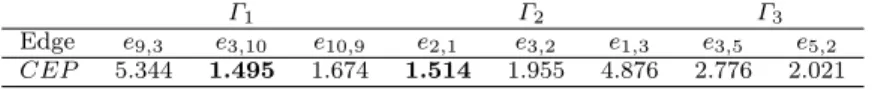
Table 2: CEP for edges in the overlapping cycles Γ2 and Γ3and non-overlapping

cycle Γ1.

Γ1 Γ2 Γ3

Edge e9,3 e3,10 e10,9 e2,1 e3,2 e1,3 e3,5 e5,2

CEP 5.344 1.495 1.674 1.514 1.955 4.876 2.776 2.021

Given the resulting weighted graph of Figure 5b, Equation 4.5 is employed to calculate the CEP (t9), which represents the criticality of the data carried by the

removed edge. In the same manner, the algorithm will calculate the CEP of the edges constituting the cycles [Γ1, Γ2, Γ3] as summarized in Table 2. Considering

this, edges e3,10 and e2,1 produce the smallest CEP which means that removing

these edges will have the smallest effect on the overall system. This results in the directed acyclic graph of Figure 5c and by extension, the graph of Figure 1b.

5 Error Propagation Approach: Experimental Evaluation

For the purpose of assessing the efficiency of the EPA methodology, we conducted a set of experiments to compare the approach with two other cycle breaking solutions in terms of system criticality. System criticality refers to the effect of removing a set of edges on the overall system. This is defined as the maximum cumulated error propagation throughout the system as a result of removing a set of edges Υ and is formally defined as,

SysCrit = max

eix∈Υ

CEP (tx) (5.1)

An industrial avionic system was taken as a reference in the choice of param-eters of these experiments. The average number of components that constitute the system as well as the graph structure of this case study were inspiration to generate the set of graphs and scenarios described below.

To ascertain that EPA does not operate haphazardly, the first approach is a random algorithm that removes a random edge from a cycle one step at a time until a DAG is obtained. The other approach is a minimum feedback arc set approximate solution. We mentioned before that finding the minimum number of edges to break all cycles in a graph is a NP-Hard problem. We implemented the approach proposed in [8], henceforth labelled MFA, that approximates the number of removed edges to break all simple cycles to the optimal minimum number.

For the purpose of these experiments, the graphs were generated using the Networkx 1.11 package [10], by taking two characteristics into account: Density and connectivity degree. Density refers to the total number of the nodes making up the graph. Connectivity degree is the ratio between the number of nodes and the total number of edges. The graphs were generated by adding nodes one at a time with an edge in either directions to one previously added node, chosen with a uniform probability.

In here, 12 scenarios were considered in which 30 random graphs were generated for every scenario with densities ranging from 10, 50, 100 to 150 nodes and 3 different degrees of connectivity with ratios [0.10, 0.25, 0.50]. The generated graphs had c number of cycles in the range c ∈ [1, 6000]. These numbers were inspired by a real case study of a full-mission simulator (FMS) in which the average number of system components ranges from 50 to 120.

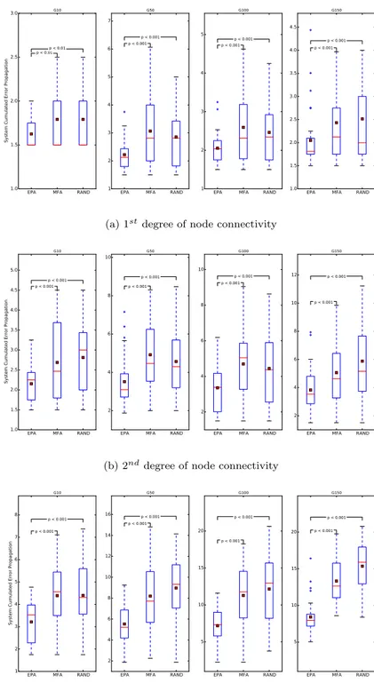
Figure 6a shows the system maximum CEP for graphs with different densities and connectivity ratio of 0.10. Although the performance of the algorithms are comparable when the density of the graphs are at 10 nodes, we notice that EPA outperforms the other methods in terms of system criticality as the density of the graphs grows. It can be seen that the Minimum Feedback Arc set solution decreases in performance and produces the most critical systems with an average SysCritM F A ∈ [2.5, 3.5] as compared to the random and EPA approach with

SysCritEP A∈ [1.8, 2.3] .

The same set of observations are noted when the connectivity between nodes is increased as shown in Figure 6b. We notice that the criticality of the system is much higher than the previous scenario, with an average SysCritEP A∈ [2.2, 3.8], which

is expected since increasing connectivity results in a more connected network and the components being more dependent on each other, which increases the chances of an error propagating to a higher number of components.

Increasing the connectivity of the nodes to the a connectivity ratio of 0.50 in Figure 6c results in the MFA performing slightly better than the random algorithm with SysCritM F A ∈ [4.3, 13.8]. However, the same scenario results in a much

superior performance from the EPA as compared to the previous scenarios with SysCritEP A∈ [2.3, 8.4].

We employed the Wilcoxon statistical test to confirm whether the results ob-tained for EPA and MFA had identical distributions. The test yielded a maximum

(a) 1st_{degree of node connectivity}

(b) 2nd_{degree of node connectivity}

(c) 3rd_{degree of node connectivity}

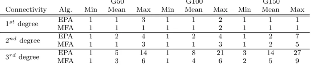
Table 3: Number of removed edges as connectivity grows.

G50 G100 G150

Connectivity Alg. Min Mean Max Min Mean Max Min Mean Max 1st_degree EPA 1 1 3 1 1 2 1 1 1 MFA 1 1 1 1 1 2 1 1 1 2nd_degree EPA 1 2 4 1 2 4 1 2 7 MFA 1 1 3 1 1 3 1 2 5 3rd _degree EPA 1 5 14 1 8 21 3 14 27 MFA 1 3 6 1 4 6 2 5 9

p-value = 2.9 · 10−3 which allows us to reject the null hypothesis H0 of identical

means.

The observations reported so far could be attributed to the fact that the main objective of the MFA solution is to minimize the number of removed edges. It would make sense that the most connected edge will be chosen by MFA to be removed. Yet, EPA will avoid these type of edges since the criticality of central edges will increase because of component dependencies.

Table 3 summarizes the number of removed edges for EPA and MFA as the connectivity degree increases. We can see that for a connectivity ratio of 0.50 and high density graphs, EPA discarded double to triple the number of edges removed by MFA. However, the system criticality was still observed to be lower for EPA than MFA as shown in Figure 6c, which supports our previous explanation. MFA removes the least number of edges but the most critical as opposed to EPA, which removes a larger number of least critical edges. That being said, for less connected graphs, the number of edges removed for EPA and MFA does not differ significantly with less critical systems in the case of EPA as seen from 6b. This could be explained by the lower degree of connectivity as well as the fact that EPA includes a step to minimize the number of removed edges.

6 Case studies

6.1 Voice-band Data Modem

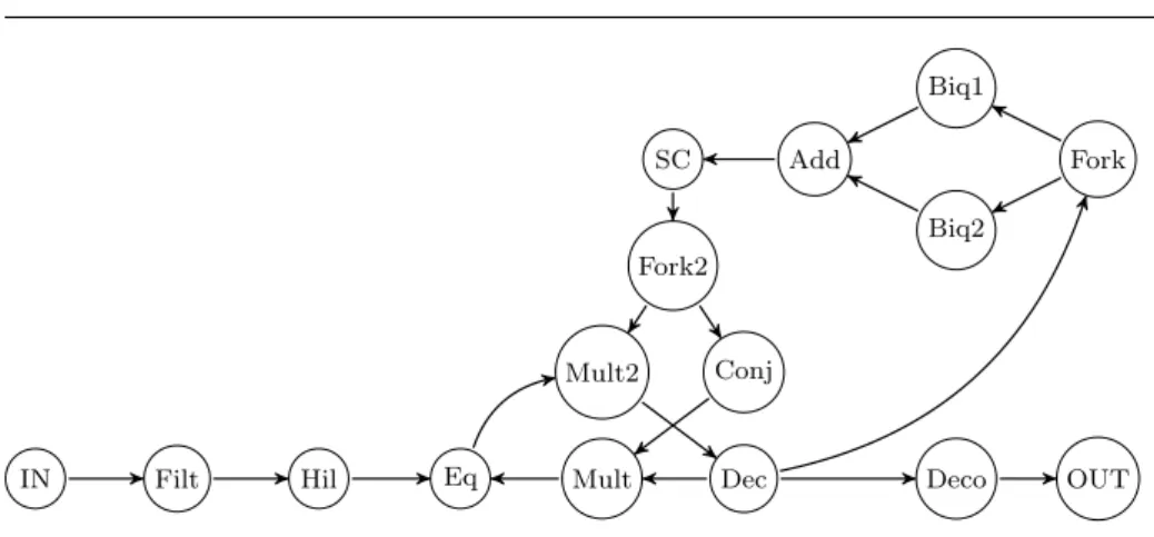
The first case study represents a voice-band data modem [2] as shown in Figure 7. This application was selected since it contains cyclic dependencies and is often employed as a benchmark to validate emerging research scheduling techniques for soft real-time systems. The graph of the modem consists of 15 components and has 5 cycles in total. Although the potential schedule start and finish points (IN, OUT) are obvious, regardless of whether their functionality is known or not, the schedule encounters a cyclic execution once it reaches the component (Eq). For such, we employ EPA to decide which edge(s) to disregard and thus, define the order in which the components will be executed. For the sake of brevity, we only show the results obtained by running the EPA algorithm on one of the cycles. Table 4 summarizes the date criticalities (CEP) when studying the edges in the cycle Γ = {Eq, Mult2, Dec, Mult}.

From Table 4, we can see that in order to have the least critical system, EPA suggests the removal of edge e(Dec,M ult) to break the cycle Γ . Running EPA on

Fork Biq1 Biq2 Add SC Fork2 Conj Mult2 Mult Dec Eq Hil Filt IN Deco OUT

Fig. 7: The directed graph of a voice-band data modem.

Table 4: CEP for edges in cycle Γ

Component Edge CEP

tEq e(M ult,Eq) 3.00

tM ult e(Dec,M ult) 2.44

tDec e(M ult2,Dec) 6.34

tM ult2 e(Eq,M ult2) 4.12

candidate edges to remove to transform the graph in Figure 7 into a DAG. From a functional point of view, the choices made by EPA do not jeopardize the correctness of the system since the component (Dec) is the decision module and is supposed to execute last in the loop. This solution agrees with many scheduling solutions found in literature for this benchmark [2, 28].

6.2 Full-Mission Simulator

Full Mission simulators are mixed-critical systems comprised of components with hard and soft deadlines. Although our approach focuses on soft real-time systems, in this section, we want to validate the accuracy of the scheduling assignment when EPA is applied.

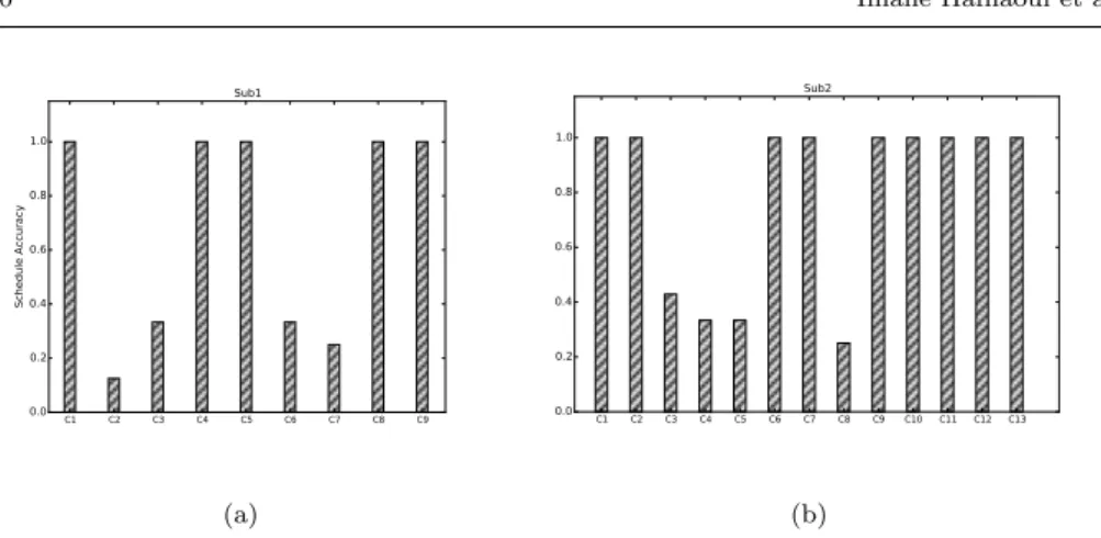
Our case study involves an industrial FMS scheduled under a modified version of RMS that consists of two subsystems: Sub1 and Sub2 consisting of 9 and 13

components respectively. The two subsystems are interconnected but the compo-nents within each subsystem execute with different rates from the compocompo-nents of the other subsystem. This means that the EPA algorithm operates on the two sub-systems separately. It is worth noting here that the current schedule with which the industrial FMS is executed was implemented by integration engineers whom take advantage of their prior expertise in the different fields and the knowledge of the components functionality, as well as, trial and error to achieve the current working state of the simulator.

In order to compare the accuracy of the system generated by EPA, we observe the accuracy of the scheduling obtained from the DAG after the transformation of EPA and the current schedule of the FMS that we label the real schedule. We

define Accusched(ti) as the degree to which the EPA scheduling matches the real

schedule for every component ti as follows:

Accusched(ti) =

P redEP A(ti)

P redReal(ti)

(6.1)

Where:

P redReal(ti) represents the number of components that are scheduled before

component ti and;

P redEP A(ti) represents the number of predecessor components that EPA

sched-uled before component ti and were scheduled as predecessors in the real schedule

as well.

Due to confidentiality agreements, we are unable to include the full details of the experiments conducted in this case study. However, we provide the outcome of the experiments henceforth.

The results obtained are summarized in Figure 8 in which the schedule accuracy obtained for both Sub1 and Sub2 following the definition in Equation 6.1 are

plotted. We can see that although the two schedules are not identical, the accuracy of the scheduled DAG obtained after EPA is relatively close to the real schedule for both subsystems. In this case study, we blindly trusted the schedule provided with the full-mission simulator (the real schedule) to be the ideal schedule. However, the real schedule sometimes gives higher execution orders to certain components even when there is no precedence requirements to be met. This can occur if other objectives are in play such as load balancing. We argue that the values provided in Figure 8 are lower bounds and that the average accuracy of the EPA schedule would increase if these cases were overlooked.

It is a good place to remind the reader that the current schedule is obtained manually after a rigorous trial and error process that involves expertise from dif-ferent fields. The fact that EPA could result in an average accuracy of 79% without requiring the knowledge of the functionalities of the components is very promis-ing, especially when dealing with such complex systems. The solution becomes more appealing to co-simulation design and early stage integration of components coming from different sources and that is by providing starting configurations that could help accelerate the process and reduce time-to-market.

7 Conclusions

Our work was driven by the current state of complex software development in avionic and automotive industries. The lack of software and architecture specifica-tions prompted us to propose an approach that offers access to the system’s task graph with no inherent knowledge of the components functionality. In this paper, we presented a methodology that makes it possible to schedule soft real-time tasks after transforming the system’s dataflow graph onto a task graph by assigning crit-icality levels to the data exchanged based on the idea of error propagation. This in turns opens access to DAG-based tools and techniques with limited knowledge about the target system. We demonstrated the efficiency of the algorithm to break cycles based on data criticality which produced the least effect on the system. As a matter of fact, the approach was able to deliver systems with criticality levels

(a) (b)

Fig. 8: Schedule accuracy for the components in (a) subsystem Sub1 and (b)

subsystem Sub2

(56± 14)% lower than other cycle breaking algorithms. Since adding new com-ponents affects the view of the system and thus increases integration cost, the approach proposed here offers the potential to test a set of configurations which will substantially reduce integration cost and offers automatic solutions to current integration issues.

Acknowledgments

This research was supported by the NSERC grant as well as CAE who provided insight and expertise that greatly assisted the research. We specially thank Patricia Gilbert, Michel Galibois and Jean-Pierre Rousseau.

References

1. Ayari, R., Hafnaoui, I., Aguiar, A., Gilbert, P., Galibois, M., Rousseau, J.P., Beltrame, G., Nicolescu, G.: Multi-objective mapping of full-mission simulators on heterogeneous distributed multi-processor systems. The Journal of Defense Modeling and Simulation: Applications, Methodology, Technology p. 1548512916657907 (2016)

2. Bhattacharyya, S.S., Murthy, P.K., Lee, E.A.: Synthesis of embedded software from syn-chronous dataflow specifications. Journal of VLSI signal processing systems for signal, image and video technology 21(2), 151–166 (1999)

3. Bonifaci, V., Marchetti-Spaccamela, A., Stiller, S., Wiese, A.: Feasibility analysis in the sporadic dag task model. In: Real-Time Systems (ECRTS), 2013 25th Euromicro Confer-ence on, pp. 225–233. IEEE (2013)

4. Buttazzo, G.: Hard real-time computing systems: predictable scheduling algorithms and applications, vol. 24. Springer Science & Business Media (2011)

5. Chandarli, Y., Fauberteau, F., Masson, D., Midonnet, S., Qamhieh, M.: Yartiss: A tool to visualize, test, compare and evaluate real-time scheduling algorithms. In: WATERS 2012, pp. 21–26. UPE LIGM ESIEE (2012)

6. Choi, J., Oh, H., Kim, S., Ha, S.: Executing synchronous dataflow graphs on a spm-based multicore architecture. In: Proceedings of the 49th Annual Design Automation Conference, pp. 664–671. ACM (2012)

7. Decker, J., Schneider, J.: Heuristic Scheduling of Grid Workflows Supporting Co-Allocation and Advance Reservation. Seventh IEEE International Symposium on Cluster Computing and the Grid (CCGrid ’07) pp. 335–342 (2007). DOI 10.1109/CCGRID.2007.56

8. Eades, P., Lin, X., Smyth, W.F.: A fast and effective heuristic for the feedback arc set problem. Information Processing Letters 47(6), 319–323 (1993)

9. Garibay-Martinez, R., Nelissen, G., Ferreira, L.L., Pinho, L.M.: Task Partitioning and Priority Assignment for Hard Real-time Distributed Systems. Journal of Computer and System Sciences 81(8), 1542–1555 (2013). DOI 10.1016/j.jcss.2015.05.005

10. Hagberg, A.A., Schult, D.A., Swart, P.J.: Exploring network structure, dynamics, and function using NetworkX. In: Proceedings of the 7th Python in Science Conference (SciPy2008), pp. 11–15. Pasadena, CA USA (2008)

11. Han, J.J., Li, Q.H.: Grid and Cooperative Computing: Second International Workshop, GCC 2003, Shanghai, China, December 7-10, 2003, Revised Papers, Part II, chap. A New Task Scheduling Algorithm in Distributed Computing Environments, pp. 141–144. Springer Berlin Heidelberg, Berlin, Heidelberg (2004)

12. Huang, Z., Shen, C.C., Doshiy, S., Thomasy, N., Duong, H.: Difficulty-level metric for cyber security training. Cognitive Methods in Situation Awareness and Decision Support (CogSIMA), 2015 IEEE International Inter-Disciplinary Conference on pp. 172–178 (2015) 13. Johnson, D.B.: Finding all the elementary circuits of a directed graph. SIAM Journal on

Computing 4(1), 77–84 (1975). DOI 10.1137/0204007

14. Kim, S.W., Park, H.S.: Periodic task scheduling algorithm under precedence constraint based on topological sort. In: 2011 8th International Conference on Ubiquitous Robots and Ambient Intelligence (URAI) (2011)

15. Kwok, Y., Ahmad, I.: Bubble scheduling: A quasi dynamic algorithm for static allocation of tasks to parallel architectures. Proceedings.Seventh IEEE Symposium on Parallel and Distributed Processing pp. 36–43 (1995). DOI 10.1109/SPDP.1995.530662

16. Kwok, Y., Ahmad, I.: Link contention-constrained scheduling and mapping of tasks and messages to a network of heterogeneous processors. Cluster Computing (2000)

17. Laalaoui, Y., Bouguila, N.: Prun-time scheduling in real-time systems: Current re-searches and artificial intelligence perspectives. Expert Systems with Applications 41(5), 2196–2210 (2014)

18. Liu, M., Becker, M., Behnam, M., Nolte, T.: A dependency-graph based priority assign-ment algorithm for real-time traffic over nocs with shared virtual-channels. In: 2016 IEEE World Conference on Factory Communication Systems (WFCS), pp. 1–8 (2016). DOI 10.1109/WFCS.2016.7496504

19. Liu, Y., Taniguchi, I., Tomiyama, H., Meng, L.: List Scheduling Strategies for Task Graphs with Data Parallelism. 2013 First International Symposium on Computing and Networking pp. 168–172 (2013). DOI 10.1109/CANDAR.2013.31

20. Morgan, M.J.: Integrated Modular Avionics for Next-Generation Commercial Air-planes. IEEE Aerospace and Electronic Systems Magazine 6(8), 9–12 (1991). DOI 10.1109/62.90950

21. Rathna Devi, M., Anju, A.: Multiprocessor Scheduling of Dependent Tasks to Minimize Makespan and Reliability Cost using NSGA-II. International Journal in Foundations of Computer Science & Technology 4(2), 27–39 (2014). DOI 10.5121/ijfcst.2014.4204 22. Roig, C., Ripoll, A., Senar, M.A., Guirado, F., Luque, E.: A new model for static mapping

of parallel applications with task and data parallelism. In: Parallel and Distributed Pro-cessing Symposium., Proceedings International, IPDPS 2002, Abstracts and CD-ROM, pp. 8–pp. IEEE (2001)

23. Sandnes, F., Sinnen, O.: Stochastic DFS for multiprocessor scheduling of cyclic taskgraphs. Lecture Notes in Computer Science 3320, 354–362 (2004)

24. Sardinha, A., Alves, T.A., Marzulo, L.A.J., Fran¸ca, F.M.G., Barbosa, V.C., Costa, V.S.: Scheduling cyclic task graphs with SCC-map. Proceedings - 3rd Workshop on Applications for Multi-Core Architecture, WAMCA 2012 pp. 54–59 (2012). DOI 10.1109/WAMCA.2012.8

25. Sebestyen, G., Hangan, A.: Genetic approach for real-time scheduling on multiprocessor systems. Intelligent Computer Communication and Processing (ICCP), 2012 IEEE Inter-national Conference on pp. 267–272 (2012). DOI 10.1109/ICCP.2012.6356198

26. Sinnen, O., Sousa, L.: List scheduling: extension for contention awareness and evaluation of node priorities for heterogeneous cluster architectures. Parallel Computing 30(1), 81–101 (2004)

27. Sriram, S., Bhattacharyya, S.S.: Embedded multiprocessors: Scheduling and synchroniza-tion. CRC press (2009)

28. Stuijk, S., Geilen, M., Basten, T.: Exploring trade-offs in buffer requirements and through-put constraints for synchronous dataflow graphs. In: Proceedings of the 43rd annual Design Automation Conference, pp. 899–904. ACM (2006)

29. Tang, Q., Basten, T., Geilen, M., Stuijk, S., Wei, J.B.: Mapping of synchronous dataflow graphs on mpsocs based on parallelism enhancement. Journal of Parallel and Distributed Computing 101, 79–91 (2017)

30. Thiele, L., Stoimenov, N.: Modular performance analysis of cyclic dataflow graphs. In: Proceedings of the seventh ACM international conference on Embedded software, pp. 127–136. ACM (2009)

31. Urunuela, R., D´eplanche, A.M., Trinquet, Y.: Storm a simulation tool for real-time mul-tiprocessor scheduling evaluation. In: Emerging Technologies and Factory Automation (ETFA), 2010 IEEE Conference on, pp. 1–8. IEEE (2010)

32. Zaki, G.F., Plishker, W., Bhattacharyya, S.S., Fruth, F.: Implementation, scheduling, and adaptation of partial expansion graphs on multicore platforms. Journal of Signal Process-ing Systems pp. 1–19 (2016)