Contents lists available atScienceDirect
Solar Energy
journal homepage:www.elsevier.com/locate/solener
Steady-state and dynamic validation of a parabolic trough collector model
using the ThermoCycle Modelica library
Adriano Desideri
a,⁎, Rémi Dickes
a, Javier Bonilla
b, Loreto Valenzuela
b, Sylvain Quoilin
a,
Vincent Lemort
aaThermodynamics Laboratory, University of Liège, Campus du Sart Tilman, B49, B-4000 Liège, Belgium
bCIEMAT-PSA, Centro de Investigaciones Energéticas, Medioambientales y Tecnológicas, Plataforma Solar de Almeria, Crta. de Senés s/n, 04200 Tabernas (Almería), Spain
A R T I C L E I N F O Keywords:
Parabolic trough collectors Dynamic validation Modelica
A B S T R A C T
Small-capacity (< 200 kWel) concentrated solar power plants has been recognized as a promising technology for
micro power applications. In particular, parabolic trough collectors have been identified as the most promising focusing technology. In this context, physics-based dynamic model of parabolic trough constitutes a significant tool for the further development of the technology, allowing to evaluate and optimize response times during transients, or to implement and test innovative control strategies. In this contribution, the dynamic model of a parabolic trough line based on the ThermoCycle Modelica library is validated against steady-state and transient experimental results from the parabolic trough test loop available at the Plataforma Solar de Almería, Spain. The simulation results are in good agreement with the measurements, both in steady-state and in transient condi-tions. The validated model is readily usable to investigate demanding dynamics-based problems for low capacity solar power systems.
1. Introduction
Recent studies have envisaged the potential of small-capacity (< 200 kWel) concentrated solar power (CSP) plants in case the future
distributed energy scenario is considered (Casati et al., 2012; Prabhu, 2006). The first documented CSP systems date back to the end of the 10th century (Butti and Perlin, 1980). Several CSP systems were de-veloped and tested during the years, and the first commercial plants were built in the 80s in California, USA (IEA-ETSAP and IRENA, 2013). The main collector technologies are point-focus single parabolic dishes, solar towers, and line-focusing parabolic troughs, vacuum tube or non-concentrating flat plate collectors (Winter et al., 1991). Non or low-concentrating configurations are particularly attractive for small-scale power units, as the lower investment costs may lead to economic via-bility. In particular, parabolic trough collectors (PTCs) are suited to supply low or medium temperature thermal energy to generate elec-tricity in combination with low-temperature organic Rankine cycle (ORC) engines (Verneau, 1978; Angelino et al., 1984).
PTCs are by far the most mature solar concentrating technology, as commercially demonstrated (Fernández-García et al., 2010). A PTC is a line-focusing parabola-shaped mirror which concentrates direct solar radiation on the absorber tube, located in the parabola’s focal line. A
heat transfer fluid (HTF) is pumped through the absorber tube ac-quiring thermal energy from the concentrated solar radiation. Parabolic trough solar thermal power plants commonly use thermal oil as HTF. These systems have been significantly improved since the first com-mercial implementation (Canada et al., 2005), and, in recent years, water has been tested as HTF in the collectors. The technology, called Direct Steam Generation (DSG), generates superheated steam directly from the collectors and presents important challenges due to phase changes in the HTF (Bonilla et al., 2015).
Due to the non-constant nature characterizing the direct solar ir-radiation, specific control strategies ensuring safe and optimal opera-tion of the CSP systems in any condiopera-tions are required. In order to design effective control strategies, the dynamics of the CSP plant must be investigated. To this end, it is fundamental to study the transient related to the solar field. In the literature, dynamic models of PTCs are mainly one-dimensional in flow direction and date back to the late 70s. The Finite Volume (FV) method is the preferred approach for the dis-cretization of the absorber tube, while Moving Boundary (MB) models have been developed for the modelling of DSG plants.
Ray (1981)presented in 1980 a non-linear dynamic model of a parabolic trough unit for DSG. The FV discretization approach was adopted and the transient responses of the model under different step
https://doi.org/10.1016/j.solener.2018.08.026
Received 28 January 2018; Received in revised form 1 August 2018; Accepted 11 August 2018
⁎Corresponding author.
E-mail address:adesideri@ulg.ac.be(A. Desideri).
0038-092X/ © 2018 Elsevier Ltd. All rights reserved.
disturbances were presented as typical results.Hirsch et al. (2005) and Eck and Hirsch (2007)developed one of the first Modelica PTC models. A FV based solar collector model of a DSG plant was introduced to-gether with a preliminary validation based on the first experimental results of the DISS facility at the Plataforma Solar de Almería (PSA), Spain. More recently, a tri-dimensional non-linear dynamic thermo-hydraulic model of a PTC was developed in Modelica and coupled to a solar industrial process heat plant modelled in TRNSYS (Silva et al., 2013). A DSG PTC model was validated against results from the DISS facility, inLobón (2014), showing a good agreement. Several dynamic models of CSP plants were developed in Modelica based on the
ThermoSysPro library (Hefni, 2014). A full scale dynamic model of a parabolic trough power plant with a thermal storage system was pre-sented inAl-Maliki et al. (2016a); simulation results were compared to experimental data from the real power plant. This work was extended inAl-Maliki et al. (2016b)including the power block and all the au-tomation processes, simulated results were compared to measured data from an existing solar power plant. A simulation model for DSG in PTCs was developed in TRNSYS (Biencinto et al., 2016), results were vali-dated with real data at the DISS facility. A thermal hydraulic RELAP5 DSG PTC model was validated against the DISS facility in Serrano-Aguilera et al. (2017), a new experimental correlation for heat losses CV control volume
TT temperature transmittance DNI direct normal irradiation ETC EuroTrough collector SF solar field
EI exogenous inputs IAM incidence angle modifier PCE percentage computational effort
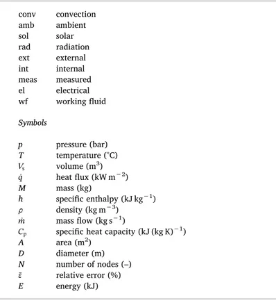
Subscripts su supply ex exhaust T temperature (°C) Vs volume (m3) q heat flux (kW m−2) M mass (kg) h specific enthalpy (kJ kg−1) density (kg m−3) m mass flow (kg s−1)
Cp specific heat capacity (kJ (kg K)−1)
A area (m2) D diameter (m) N number of nodes (–) ¯ relative error (%) E energy (kJ) 1 2 3 i-1 i i+1 N-1 N … …
(a)
(b)
Fig. 1. Parabolic trough collector model in ThermoCycle. (a): One-dimensional finite-volume modelling of the PTC. (b): Object diagram of the solar collector model
was also provided. A non-linear dynamic model of once-trough DSG PTCs was developed inGuo et al. (2017)and transfer functions of outlet fluid temperature and mass flow rate were derived.
The present work focuses on the steady-state and dynamic valida-tion of a parabolic trough collector model included in the open-source ThermoCycle Modelica library, for the modelling of small thermo-hy-draulic system (Quoilin et al., 2014). The main contribution consists in a through validation of the PTC model against experimental data col-lected at the “HTF Loop” facility in Almería, Spain. The model is a detailed implementation of the Forristal approach (Forristall, 2003), it is highly customizable and can be used to model any kind of PTC solar field. The paper is organized as follows: in Section2the PTC model is described. In Section3the experimental campaign is outlined. Section4 reports the results for the steady-state and dynamic validation analysis. In Section5critical aspects when modelling parabolic trough collectors are discussed. The main conclusions are drawn in Section6.
2. Parabolic trough collector modelling
The parabolic trough model is developed in the Modelica language (Elmqvist, 1978) and is part of the open-source ThermoCycle library (Quoilin et al., 2014). As depicted in Fig. 1a, the model relies on a finite-volume approach for the modelling of the heat collection element (HCE), which is discretized along its axial axis in N constant and uni-form control volumes (CV). The one-dimensional modelling method is justified by the large ratio between the diameter and the length of the HCE. Following the object-oriented formalism of Modelica, the PTC model is built by interconnecting two sub-components, i.e. the Flow1D and the SolAbs models. These two are linked together through a thermal port as depicted inFig. 1b.
The Flow1D component simulates the fluid flow in the HCE. In each CV, both mass and energy balances are solved assuming an in-compressible fluid and a static momentum balance. Considering the abovementioned assumptions, the final conservation law formulations for each CV are reported in Eqs.(1)–(3), with pressure, p, and specific enthalpy, h, as dynamic state variables.
= = = + dM dt m m dM dt V h dh dt p dp dt 0 with · · su ex (1) = + + V dh dt m h h m h h V dp dt A q ( ) ( ) · su su ex ex conv fl, (2) = psu pex (3)
The “su” (supply) and “ex” (exhaust) subscripts denote the nodes variable of each CV, A is the lateral surface through which the heat flux
qconv fl, is transferred to the fluid and V is the constant volume of each CV. An upwind discretization scheme is selected. / h and / p are treated as thermodynamic properties of the fluid and are directly computed by the open-source CoolProp library, featuring high accuracy Helmholtz energy-based equation of states (Bell et al., 2014). The
So-lAbs submodel simulates the effective thermal energy transferred from
the ambient through the HCE to the fluid. The model is built upon Forristall steady-state equations (Forristall, 2003) with the dynamic 1D radial energy balance around the HCE, seeFig. 2. The model relies on physics-based equations and accounts for:
•
conduction and thermal energy accumulation in the metal pipe;•
convection and radiation between the glass envelope and the metalpipe;
•
conduction and thermal energy accumulation in the glass envelope;•
radiation and convection losses to the environment.The environmental parameters, i.e. the direct normal irradiation, DNI, the solar radiation incidence angle, incid, the ambient
tempera-ture, Tamb, and the wind speed,vwind, are inputs to the SolAbs sub-model.
The selected modelling approach allows simulating the relation be-tween the environmental parameters and the axial temperature dis-tribution along the absorber tube. The thermal power transferred to the fluid, qconv,fl, the thermal losses to the environment,qconv,amb+ qrad,amb,
and the temperatures of both the metal pipe, Tt, and the glass envelope,
Tg, can then be evaluated. Temperatures, heat transfer coefficients, and
thermodynamic properties are assumed uniform around the cir-cumference of the HCE (1-D model). Thermal losses through the sup-port brackets are neglected and solar absorption in the tube and the glass envelope is treated as a linear phenomenon. Unlike Forristall’s original model, the energy balances in the glass envelope and the metal pipe are calculated accounting for their thermal capacity as shown in Eqs.(4)and(5). = + C dT dt q D q D g p g g
int g int g ext g ext g
, , , , , (4)
= +
C dT
dt q D q D
t p t, t int t int t, , ext t ext t, , (5)
For a detailed description of the modelling approach and heat transfer coefficient calculation, the interested reader can refer to Forristall (2003) and Desideri (2016).
3. Measurements and experiments
3.1. Experimental facility
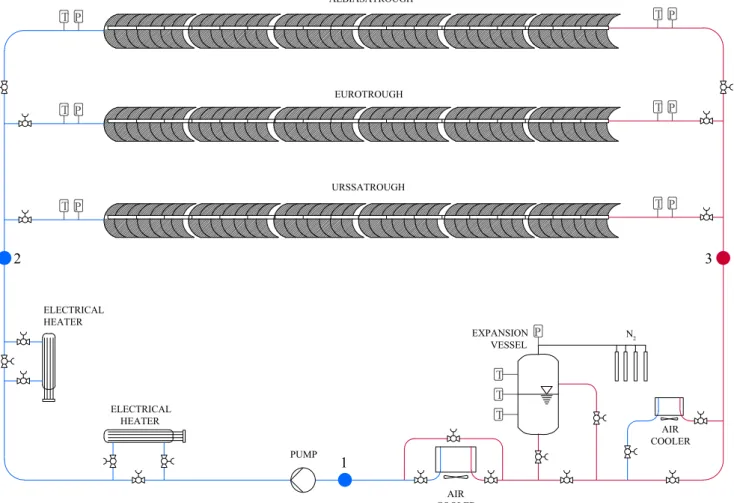
The experiments were carried out at the HTF Loop, at the Plataforma Solar de Almería, Spain. An aerial view of the HTF system is shown inFig. 3. The solar field was characterized by three parallel lines of parabolic trough collectors (PTC) from different manufacturers Al-biasaTrough, EuroTrough and UrssaTrough. The system was a closed loop, with an East–West orientation and it was charged with the thermal oil Syltherm 800 (Dow Oil and Gas, 1997). The process flow diagram of the HTF facility is shown inFig. 4. Looking at the bottom of Fig. 4it is possible to recognize the pump which drove the fluid, in liquid state, through one of the three parallel PTC lines of the solar field. The fluid was heated from (2) to (3) absorbing the solar energy reflected by the collectors to the receiver tubes. At the outlet of the collectors, the fluid was cooled down by air-cooler II characterized by a maximum thermal capacity of 400 kWth. Once cooled down the oil
reached the pump suction port (1). A 1 m3expansion vessel with
Ni-trogen (N2) inertization, located in between the two air coolers, was
used to regulate the loop pressure, limited to 18 bar. In the whole cir-cuit, oil was maintained in liquid state. Two electric heaters installed at
Fig. 2. Energy balance around the HCE. In blue the glass envelope, in grey the
metal pipe and in white the vacuum between the two. Heat transfer is high-lighted with red arrows. (For interpretation of the references to color in this figure legend, the reader is referred to the web version of this article.)
the pump outlet allowed controlling the temperature at the inlet of the PTC lines. A mass flow meter at the outlet of the pump was used to measure the oil mass flow rate. The temperatures at the inlet and at the outlet of the PTC were measured with PT100 (TT) sensors, character-ized with an uncertainty of ± 1 K (Sallaberry et al., 2017). The direct normal irradiation (DNI) was measured with a pyrheliometer model CH1 by Kipp and Zonen (1997). Ambient temperature and the wind speed were acquired from a weather station installed nearby the perimental facility. A sampling time of 5 s was set to acquire the ex-perimental data and LabView was used for data visualization. During the experimental campaign, the EuroTrough collectors (ETC) line was tested. The ETC line was composed by 6 EuroTrough modules con-nected in series and 18 prototype receiver tubes from a Chinese
manufacturer for a total length of 70.8 m and a net aperture area of 409.9 m2.
3.2. Steady-state and dynamic experiments
In order to characterize the performance of the ETC line, 24 steady-state points were collected at different operating conditions, by varying the pump speed and the temperature at the inlet of the ETC, for a total of 5 days of testing. The system was run in stable conditions (TT tem-perature variations below 2 °C) for 10 min and the steady-state point was recorded by averaging the measurements over a period of 6 min. The acquired data were used to calibrate and validate the model in steady-state. In order to characterize the dynamic performance of the
P T T P P T T P P T T P P T T T PUMP
1
AIR COOLER AIR COOLER EXPANSION VESSEL URSSATROUGH EUROTROUGH ALBIASATROUGH N2 ELECTRICAL HEATER ELECTRICAL HEATER2
3
Fig. 4. Process flow diagram of the HTF facility with the relative sensors position. Fig. 3. Aerial view of the HTF loop at PSA, Almería.
ETC, step changes were applied to the pump speed and the ETC inlet temperature. InTable 1, the working conditions of the main variables and of the external ambient parameters during the experimental cam-paign are reported. The dynamic validation was based on three specific sets of experiments:
•
MFE – Oil mass flow change experiment: a step change was imposedto the oil mass flow rate at the inlet of the ETC by varying the pump speed upwards or downwards starting from a steady-state condition.
•
TE – Oil inlet temperature change experiment: the oil temperature atthe inlet of the ETC was varied by shutting down the air cooler starting from a steady-state condition.
•
SBE – Solar beam radiation change experiment: a step change to thesolar beam radiation collected by the receiver was imposed down-wards and updown-wards by defocusing and focusing the trough collec-tors.
4. Simulation results and experimental validation
The steady-state and dynamic validation of the ETC dynamic model described in Section2is presented in this section. The model is com-pared against experimental data acquired on the HTF Loop facility at
the Plataforma Solar de Almería (PSA), Spain.
4.1. Initial conditions, model inputs, and parameters
In order to compare the experimental data with the modelling re-sults a simulation framework was defined. A schematic of the solar field (SF) model is shown inFig. 5. It comprised a mass flow source and a pressure sink connected to the fluid connectors of the SF model. The exogenous inputs (EI) imposed to the ETC model and the relative units are listed inTable 2. The SF model was parameterized based on the data-sheets of the EuroTrough collector and the receiver. The incidence
Table 1
Range of operation of the ETC main variable and of the external ambient condition during the experimental campaign.
Variable moil,su pSF su, Toil,su Toil,ex DNI Tamb vwind
Unit [kg s−1] [bar] [°C] [°C] [W m−2] [°C] [m s−1] Min 1.55 12.96 150.05 170.21 593.95 26.23 0 Max 5.03 16.07 304.48 352.28 883.72 33.16 11.23
Fig. 5. Modelica model of the ETC line installed at the HTF Loop facility from
the Dymola graphical user interface (GUI).
Table 2
List of exogenous inputs (EI) imposed to the SF model.vwind: wind speed, incid:
solar radiation incidence angle, Tamb: ambient temperature, DNI: direct normal
irradiation, Fvector: vector for defocusing action, moil su, : oil mass flow at SF inlet,
Toil su, : oil temperature at SF inlet, pex: oil pressure at SF outlet
EI vwind incid Tamb DNI Fvector moil,su Toil,su pex
Unit [m s−1] [Rad] [°C] [W m−2] [–] [kg s−1] [°C] [bar]
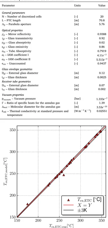
Table 3
Values of the parameters for the SF Modelica model.
Parameter Units Value
General parameters
N – Number of discretized cells [–] 20
L – PTC length [m] 70.8 Ap– Parabola aperture [m] 5.76 Optical properties cl– Mirror reflectivity [–] 0.9388 gl– Glass transmissivity [–] 0.92 gl– Glass absorptivity [–] 0.02 gl– Glass emissivity [–] 0.86 tu– Tube Absorptivity [–] 0.7919
aI– IAM coefficient I [–] 4.11e 3
aII– IAM coefficient II [–] 5.513e5
un– Unaccounted [–] 0.9437
Glass envelope geometries
Dgl– External glass diameter [m] 0.12
tgl– Glass thickness [m] 0.0025
Receiver tube geometries
Dtu– External glass diameter [m] 0.07
ttu– Glass thickness [m] 0.002
Vacuum properties
pvacuum– Vacuum pressure [bar] 1.333e7
– Ratio of specific heats for the annulus gas [–] 1.39
mol– Molecular diameter for the annulus gas [m] 3.53e 10
kstd– Thermal conductivity at standard pressure and
temperature [W m
−1K−1] 0.02551
Fig. 6. Parity plot for the ETC model outlet temperature compared against the
angle modifier (IAM), required for the optical efficiency calculation, was computed with an empirical equation as:
= +
IAM 1 a· a ·
cos ,
I incid II incid2
incid (6)
where incidis the incidence angle of solar radiation and a aI IIare two
empirical parameters derived through experimental data reported in (Sallaberry et al., 2016), following the methodology presented in (Valenzuela et al., 2014). In order to consider unaccounted optical ef-fects, e.g., dirt on the parabolic mirrors and tube receivers, the
parameter unwas included in the calculation of the optical efficiency. Its
value was obtained through a least square optimization routine aimed at minimizing the error between the simulated SF outlet temperature and the measured one over a six minutes interval of the initial steady-state con-dition characterizing the first day of testing, seeFig. 8. InTable 3, the values assigned to the parameters of the SF model are reported.
In the SF model, the density, specific heat capacity and thermal conductivity of the glass and the metal envelopes were considered as temperature dependent. The heat transfer coefficient was computed based on the Gnielinski single phase correlation (Gnielinski, 2010). The thermal oil, Syltherm 800, flowing through the receiver was modelled
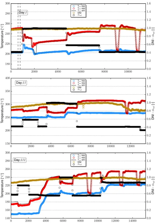
Fig. 7. Simulation and experimental results plotted versus time for: (a) MFE – Mass flow change experiment [DNImax: 822.76 W m2, mwf,max: 4.41 kg m1]. (b) TE –
inlet ETC temperature change experiment [DNImax: 842.2 W m2, mwf,max: 4.82 kg m 1]. (c) SBE – solar beam radiation change experiment [DNImax: 804.15 W m2,
mwf,max: 4.92 kg m1]. The measured inlet and outlet ETC temperatures and the outlet SF model temperature are plotted on the left abscissa. The normalized DNI and
as an incompressible fluid using the TableBased framework of the Modelica Standard library, i.e. no mass accumulation was considered.
4.2. Results: steady-state validation
The SF model was compared against 24 steady-state experimental points. The data were acquired at different ETC inlet temperatures, by varying the pump rotational speed and the thermal input of the heaters and air coolers. InFig. 6, the model predictions for the temperature at the outlet of the ETC line are plotted versus the experimental values. The SF model is able to reproduce the measured data points with a good agreement. The temperature at the outlet of the collectors is char-acterized by an accuracy within 3 °C for most of the tested conditions. For an outlet temperature below 200 °C, an accuracy within 4 °C is
found. As the ETC outlet temperature decreases, an increasing dis-crepancy between experimental and simulated results is registered. This might be related to the optical effect parameter un, which is computed
for an outlet temperature of 250 °C, seeFig. 8.
4.3. Results: dynamic validation
The SF Modelica model was run on Dymola2017. The Differential Algebraic System Solver (DASSL) (Petzold, 1983) was selected as nu-merical solver, setting the relative tolerance to 10 4. In order to increase
the model robustness and decrease the computational time, the mea-sured variables imposed as exogenous inputs to the SF model, see Table 2, were approximated by a spline function in the Modelica/Dy-mola simulation environment.
InFig. 7, the simulated ETC outlet temperature is plotted versus time and compared against the measured data for each of the three performed dynamic experiments. On the left abscissa the measured ETC inlet and outlet temperatures and the simulated ETC outlet temperature are plotted versus time. On the right abscissa the DNI and oil mass flow rate, mwf, normalized with respect to the maximum value reached
during the day (DNImax,mwf,max), are reported. For all the plots, it is
possible to see how the DNI was characterized by variation smaller than 2%.
InFig. 7a, the results of the MFE experiment and simulation are reported. Starting from a steady-state condition two consecutive steps of the same magnitude upwards and downwards were imposed to the pump rotational speed at t = 450 s and t = 1430 s respectively. As the pump rotational speed was raised at t = 450 s, the velocity and pressure of the fluid in the high pressure line increased. This resulted in an oil
mass flow rate,mwf, increment of about 40% in around 60 s. The
in-crease in oil mass flow rate caused a drop in the temperature at the outlet of the ETC,Tex. The temperature drop was registered at around
t = 500 s, 50 s after the oil mass flow rate changed. This was due to the time required by the oil mass flow rate to reach the outlet of the 70.8 m long receiver tubes. During the experiments, the ETC inlet temperature, Tsu, was maintained constant by manually manipulating the air cooler
and electrical heaters power. When a step upwards was imposed to the oil mass flow rate, asTsuwas expected to drop, the air cooler power and
the electrical heaters power were manually modified. This led to a small bump of 2 K in the temperature as it is shown inFig. 7a. The same phenomena in the opposite direction took place when the pump speed was decreased. The ETC outlet temperature presented a symmetrical trend for the upwards and downwards oil mass flow rate change. The SF model was able to well predict the experimental trend both for the
upward and downward steps, and was characterized by a time constant slightly smaller than the real system.
InFig. 7b, the TE experiments and simulation results are reported. Starting from a steady-state condition the air-cooler was turned off at t = 900 s. This resulted in an increase ofTsuand a consequent growth of Texdelayed by around 100 s due to the time required by the oil mass flow
to travel through the tube receiver. The shut-down of the oil-cooler did not allow to impose a step toTsuwhich increased with a slow first order trend.
The large time constant characterizingTsudefined the change of the outlet
ETC temperature. The SF model was able to correctly predict the experi-mental results including the delay characterizing theTextrend.
InFig. 7c, the SBE experiments and simulation results are shown. Starting from a steady-state condition the ETCs were defocused at t = 360 s, such that no solar radiation was reflected to the receiver tubes. This caused a sudden decrease ofTexwhich reached theTsuvalue
in about 200 s. The ETCs were focused again at t = 650, bringingTex
back to its initial value. During the experiment, the oil mass flow rate andTsuwere kept constant. The latter was maintained at its initial value
by manually manipulating the power of the two electrical heaters in-stalled after the pump. This resulted in a small bump of less then 4 K at t = 700 s, after the collectors were focused. TheTexwas characterized
by a symmetrical behavior during the focusing-defocusing experiment, as the thermal energy losses were relatively small. The SF model was able to replicate the trend and presented a slightly smaller time con-stant than the real system.
It can be concluded that the SF Modelica model was capable of pre-dicting the physical phenomena characterizing the solar field dynamics during the three performed experiments, and can be considered validated. InFigs. 8 and 9, the simulation and experimental results for the six days of testing are reported. InFig. 8- Day I, the three minutes time over which the unparameter was optimized are highlighted by two
vertical black dotted lines. During Day VI, continuous changes were imposed on the HTF facility to test the model during highly variable conditions. As shown inFig. 9– Day VI, the model is able to correctly predict the collector outlet temperature despite the extreme variations.
4.4. Simulation tool
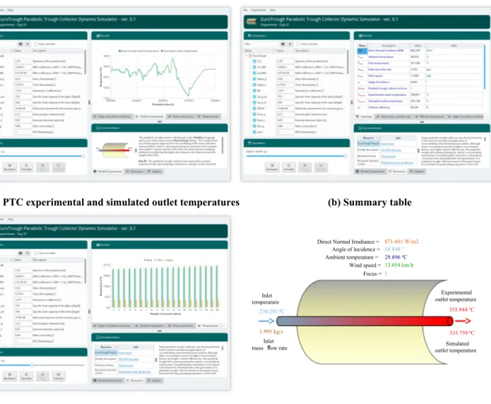
A simulation application of the developed PTC model was built as a tool to reproduce the results presented in Section4. The simulator is open source and is freely available at https://ciemat-psa.gitlab.io/surf-simulator/projects/EuroTrough. Currently, there are binary versions for Linux and Windows platforms. This tool allows users to easily re-produce the results presented in the validation section. Furthermore, users can change the PTC configuration and evaluate how such changes affect the performance and results.
InFig. 10, a graphical overview of the simulation tool is reported. The application includes the Modelica model exported following the Functional Mock-up Interface (FMI) standard, input files, experimental results, diagrams, and documentation.
(a) PTC experimental and simulated outlet temperatures
(b) Summary table
(c) Fluid, tube and glass temperatures in each CV
Ambient temperature = 29.896 ºC
270.297 ºC 1.995 kg/s
Direct Normal Irradiance = 871.601 W/m2
335.759 ºC
Focus =1
Wind speed =13.054 km/h
335.944 ºC
Simulated outlet temperatureExperimental
outlet temperature Inlet temperature Inlet mass ow rate Angle of incidence = 18.848 º
(d) Diagram
Fig. 10. EuroTrough simulation tool.Each one of the six operating days, discussed in Section4.3(Day I
-IV), can be simulated. Model parameters, reported inTable 3, are ac-cessible. Once the simulation is complete, the user can evaluate the results at any particular time instant, as shown inFig. 10b. The simu-lated results can be compared against experimental data (seeFig. 10a).
Information on each CV is provided, as shown inFig. 10c where fluid, tube and glass temperatures for a particular point in time are reported. Furthermore, the tool includes a diagram of the process, displaying information about a particular point in time of the simulation (see Fig. 10d).
5. Discussion
This work aims at proposing a tool to analyze the unsteady opera-tions of parabolic trough collectors, with a special attention to the following characteristics:
•
Satisfactory accuracy for engineering applications•
Low computational timeThe SF model is based on the finite volume method, characterized by a trade-off between model accuracy and computational time: in-creasing the number of CVs leads to better accuracy but negatively affects the computational effort.
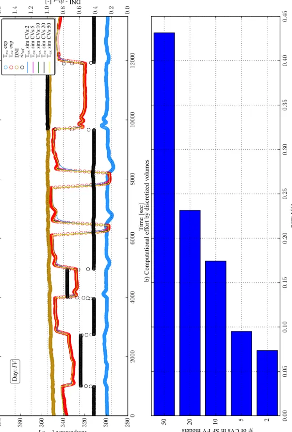
In order to investigate the effect of the level of discretization on the performance of the SF model when compared to the experimental re-sults, a parametric analysis was performed. The SF model, discretized with a number of control volumes (CVs) varying from 1 to 50, was simulated to replicate the experimental data of Day IV, seeFig. 9. The results are displayed in Fig. 11a where the simulated SF outlet tem-perature for the different levels of discretization is plotted versus time and compared against the measured experimental data on the left ab-scissa. On the right abscissa the nominal DNI and oil mass flow rate are plotted. Overall, as the level of discretization increased the SF outlet temperature got closer to the measurements data. From 10 to 50 CVs the improvement in model accuracy was negligible. On the other hand, the 5 CVs and 1 CVs SF model presented a slower time constant com-pared to the real system and were not able to properly predict the different undershoot and overshoot characterizing the measured outlet ETC temperature when the boundary conditions where changed, e.g., step change in the mass flow (MFE) or defocusing-focusing (SBE).
InFig. 11b, the percentage computational effort (PCE) defined in Eq.(7)as the ratio of the computational time (TimeComp) with respect
to the simulated time (TimeReal), is plotted for each simulation result.
All the simulations were characterized by a much shorter time com-pared to the real simulated time. This is related to the remarkably simple simulation framework on which the modelling results were based on (see Section4.1).
=
PCE Time Time ·100
Comp
Real (7)
The computational time increased exponentially with the increase of number of CVs, with the 1 and 5 CVs SF models being one order of magnitude faster than the higher discretized model.
In order to assess the discrepancy between the different CVs dis-cretization levels, the total energy absorbed by the thermal oil in the ETC collectors,Ewf, was computed as the integral of the thermal power
over the simulated time, over 4 h, and compared with respect to the 50 CVs model, taken as a reference. The percentage relative error ¯ for each SF model was computed as:
=
k E E
E k
¯ ( ) 100·| wf,50CVs wf,k| [1, 5, 10, 20].
wf,50CVs (8)
The results are reported inTable 4. As it is possible to see, the overall percentage relative error on the total energy absorbed by the fluid over
4 h of simulation with respect to the 50 CVs SF reference model was negligible for all the tested levels of discretization.
6. Conclusions
This work presents a dynamic model for the modelling of parabolic trough collectors. The proposed model is open source and it is included in the ThermoCycle Modelica library. A validation of the model is presented against experimental data acquired at the HTF facility at the Plataforma Solar de Almería (PSA), Spain. Steady-state and dynamic experimental data were obtained at different operating conditions by varying the pump rotational speed, the heater and cooler set-points and by focusing-defocusing the collectors. A first validation was performed against 24 steady-state data points. A second dynamic validation was carried out with 3 sets of experiments by varying the oil mass flow rate (MFE), the oil inlet temperature (TE) and the solar beam radiation (SBE). The main outcomes of this study are reported hereunder.
•
The steady-state validation shows a good agreement between ex-perimental and simulated temperature at the outlet of the collectors. Most of the data are reproduced with an accuracy below 3 °C. For temperature below 200 °C, the temperature is predicted with a 4 °C error.•
The simulation results obtained for the oil mass flow (MFE), the oil inlet temperature (TE) and the solar beam radiation (SBE) experi-ments showed a good overlap with the experimental results. The developed solar field model structure proves to be effective to pre-dict the dynamic of a real line of solar collectors.•
A minimum discretization level of 20 CVs was found to be a good compromise between model accuracy and simulation speed if the ETC outlet temperature had to be precisely predicted, e.g., the SF model is used as a reference to develop and test model based control strategies.•
In light of the obtained results a lumped SF model is recommended if the performance of the ETC collectors are analysed on a daily or longer time frame. This approach allows to significantly decrease the computational time while maintaining a satisfying level of ac-curacy.•
A simulation tool was built to reproduce the dynamic validation results presented in the paper. The tool is open-source and can be used as a reference for modelling parabolic trough collectors. It was proven that the modelling approaches adopted led to sa-tisfactory results for the simulation of parabolic trough collector sys-tems. The proposed solar collector model together with the test cases is released as open-source and is available in the latest version of the ThermoCycle library. It should be noted that the model is not suitable for the simulation of start-up or shut-down of the collectors, as the proposed finite volume approach does not handle zero flow conditions. Future work entails the adoption of the developed model to simulate small-scale CSP plants based on ORC technology, in order to investigate different control strategies.Acknowledgements
The results presented in this paper have been obtained within the frame of the SFERA II project (EU FP7 grant agreement No. 312643). These financial supports are gratefully acknowledged. Furthermore, the authors want to thank the financial support received from the BRICKER project (www.bricker-project.com). This project has received funding from the European Unions Seventh Framework Programme for re-search, technological development and demonstration under grant agreement No. 609071. The information reflects only the authors view and the Commission is not responsible for any use that may be made of the information it contains.
Table 4
Total energy percentage relative error for the different levels of discretization of the SF model. Model ¯[%] SF CVs 1 0.5 SF CVs 5 0.18 SF CVs 10 0.08 SF CVs 20 0.03
Bonilla, J., Dormido, S., Cellier, F.E., 2015. Switching moving boundary models for two-phase flow evaporators and condensers. Commun. Nonl. Sci. Num. Simul. 20 (3), 743–768.
Butti, K., Perlin, J., 1980. A golden thread: 2500 years of solar architecture and tech-nology.
Canada, S., Cohen, G., Cable, R., Brosseau, D., Price, H., 2005. Parabolic trough organic rankine cycle solar power plant. National Renewable Energy Laboratory, vol. 1, January 2005, pp. 1–2.
Casati, E., Desideri, A., Casella, F., Colonna, P., 2012. Preliminary assessment of a novel small csp plant based on linear collectors, ORC and Direct Thermal Storage. In: SolarPaces Conference.
Desideri, A., 2016. Dynamic modeling of organic rankine cycle power systems. Dow Oil and Gas, 1997. Syltherm 800 Heat Transfer Fluid. Tech. Rep.; DOW. Eck, M., Hirsch, T., 2007. Dynamics and control of parabolic trough collector loops with
direct steam generation. Solar Energy 81 (2), 268–279.https://doi.org/10.1016/j. solener.2006.01.008.
Elmqvist, H., 1978. A Structured Model Language for Large Continous Systems. Ph.D. thesis; Lund Institute of Technology.
Fernández-García, A., Zarza, E., Valenzuela, L., Pérez, M., 2010. Parabolic-trough solar collectors and their applications. Rene. Sustain. Energy Rev. 14 (7), 1695–1721.
https://doi.org/10.1016/j.rser.2010.03.012.
Forristall, R., 2003. (U.S.) N.R.E.L, of Energy U.S.D, of Energy. Office of Scientific U.S.D, Information T. Heat Transfer Analysis and Modeling of a Parabolic Trough Solar Receiver Implemented in Engineering Equation Solver. National Renewable Energy Laboratory.
Forristall, R., 2003. Heat Transfer Analysis and Modeling of a Parabolic Trough Solar Receiver Implemented in Engineering Equation Solver. Tech. Rep. October; National Renewable Energy Laboratory.
Gnielinski, V., 2010. Heat Transfer in Pipe Flow. VDI Heat Atlas 691–700.https://doi. org/10.1007/978-3-540-77877-6_34.
Guo, S., Liu, D., Chu, Y., Chen, X., Xu, C., Liu, Q., et al., 2017. Dynamic behavior and transfer function of collector field in once-through dsg solar trough power plants. Energy 121 (Supplement C), 513–523.https://doi.org/10.1016/j.energy.2017.01.
Prabhu, E., 2006. Solar Trough Organic Rankine Electricity System ( STORES ) Stage 1: Power Plant Optimization and Economics. Tech. Rep. March. doi:NREL/SR-550-39433.
Quoilin, S., Desideri, A., Wronski, J., Bell, I.H., Lemort, V., 2014. ThermoCycle: a Modelica library for the simulation of thermodynamic systems. In: Proceedings of the 10thInternational Modelica Conference.
Ray, A., 1981. Nonlinear dynamic model of a solar steam generator. Solar Energy 26 (4), 297–306.
Sallaberry, F., Valenzuela, L., de Jalón, A.G., Leon, J., Bernad, I.D., 2016. Towards standardization of in-site parabolic trough collector testing in solar thermal power plants. AIP Conf. Proc. 1734, 130019-1–130019-8.https://doi.org/10.1063/1. 4949229.
Sallaberry, F., Valenzuela, L., Palacin, L.G., 2017. On-site parabolic-trough collector testing in solar thermal power plants: experimental validation of a new approach developed for the iec 62862-3-2 standard. Solar Energy 155, 398–409.https://doi. org/10.1016/j.solener.2017.06.045.
Serrano-Aguilera, J., Valenzuela, L., Parras, L., 2017. Thermal hydraulic relap5 model for a solar direct steam generation system based on parabolic trough collectors operating in once-through mode. Energy 133 (Supplement C), 796–807.https://doi.org/10. 1016/j.energy.2017.05.156.
Silva, R., Pérez, M., Fernández-Garcia, A., 2013. Modeling and co-simulation of a para-bolic trough solar plant for industrial process heat. Appl. Energy 106 (Supplement C), 287–300.https://doi.org/10.1016/j.apenergy.2013.01.069.
Valenzuela, L., López-Martín, R., Zarza, E., 2014. Optical and thermal performance of large-size parabolic-trough solar collectors from outdoor experiments: a test method and a case study. Energy 70, 456–464.https://doi.org/10.1016/j.energy.2014.04. 016.
Verneau, A., 1978. L’emploi des fluides organiques dans les turbines solaires. Entropie 9–18.
Winter, C.J., Sizmann, R.L., Hull, L.V., 1991. Solar Power Plants. Springer Verlag.https:// doi.org/10.1007/978-3-642-61245-9.