https://doi.org/10.5194/tc-13-1349-2019
© Author(s) 2019. This work is distributed under the Creative Commons Attribution 4.0 License.
Uncertainty quantification of the multi-centennial response
of the Antarctic ice sheet to climate change
Kevin Bulthuis1,2, Maarten Arnst1, Sainan Sun2, and Frank Pattyn2
1Computational and Stochastic Modeling, Aerospace and Mechanical Engineering, Université de Liège,
Allée de la Découverte 9, Quartier Polytech 1, 4000 Liège, Belgium
2Laboratoire de Glaciologie, Department of Geosciences, Environment and Society, Université Libre de Bruxelles,
Av. F.D. Roosevelt 50, 1050 Brussels, Belgium
Correspondence: Kevin Bulthuis ([email protected]) Received: 15 October 2018 – Discussion started: 10 December 2018
Revised: 12 March 2019 – Accepted: 6 April 2019 – Published: 24 April 2019
Abstract. Ice loss from the Antarctic ice sheet (AIS) is ex-pected to become the major contributor to sea level in the next centuries. Projections of the AIS response to climate change based on numerical ice-sheet models remain chal-lenging due to the complexity of physical processes involved in ice-sheet dynamics, including instability mechanisms that can destabilise marine basins with retrograde slopes. More-over, uncertainties in ice-sheet models limit the ability to provide accurate sea-level rise projections. Here, we apply probabilistic methods to a hybrid ice-sheet model to investi-gate the influence of several sources of uncertainty, namely sources of uncertainty in atmospheric forcing, basal slid-ing, grounding-line flux parameterisation, calvslid-ing, sub-shelf melting, ice-shelf rheology and bedrock relaxation, on the continental response of the Antarctic ice sheet to climate change over the next millennium. We provide probabilis-tic projections of sea-level rise and grounding-line retreat, and we carry out stochastic sensitivity analysis to determine the most influential sources of uncertainty. We find that all investigated sources of uncertainty, except bedrock relax-ation time, contribute to the uncertainty in the projections. We show that the sensitivity of the projections to uncertain-ties increases and the contribution of the uncertainty in sub-shelf melting to the uncertainty in the projections becomes more and more dominant as atmospheric and oceanic tem-peratures rise, with a contribution to the uncertainty in sea-level rise projections that goes from 5 % to 25 % in RCP 2.6 to more than 90 % in RCP 8.5. We show that the signifi-cance of the AIS contribution to sea level is controlled by the marine ice-sheet instability (MISI) in marine basins, with
the biggest contribution stemming from the more vulnerable West Antarctic ice sheet. We find that, irrespective of para-metric uncertainty, the strongly mitigated RCP 2.6 scenario prevents the collapse of the West Antarctic ice sheet, that in both the RCP 4.5 and RCP 6.0 scenarios the occurrence of MISI in marine basins is more sensitive to parametric uncer-tainty, and that, almost irrespective of parametric unceruncer-tainty, RCP 8.5 triggers the collapse of the West Antarctic ice sheet.
1 Introduction
The Antarctic ice sheet (AIS) is the largest reservoir of freshwater on Earth ( ∼ 60 m sea-level equivalent, Fretwell et al., 2013; Vaughan et al., 2013) and has the potential to become one of the largest contributors to sea level in the next centuries. Yet, studies such as the IPCC Fifth Assess-ment Report (AR5) (Stocker et al., 2013) and Kopp et al. (2014) have identified the magnitude of the AIS response as the largest source of uncertainty in projecting sea-level rise, when compared with other contributors such as thermal ex-pansion, glaciers and the Greenland ice sheet. Recent obser-vations (Shepherd et al., 2018) have shown an acceleration in the rate of ice loss from the Antarctic ice sheet, especially in West Antarctica, where an irreversible retreat may be un-derway in the Amundsen Sea Embayment as a consequence of a marine ice-sheet instability (MISI) (Favier et al., 2014; Joughin et al., 2014; Rignot et al., 2014).
Assessing the future response of the Antarctic ice sheet requires numerical ice-sheet models amenable to large-scale
and long-term simulations and quantification of the impact of modelling hypotheses and parametric uncertainty. So far, there exist only a limited number of projections (Golledge et al., 2015; Ritz et al., 2015; DeConto and Pollard, 2016; Schlegel et al., 2018) for the whole Antarctic ice sheet on a (multi-)centennial timescale. These projections show similar trends for the next centuries, but they differ in the magni-tude of the mass loss they predict, with differences and un-certainty ranges that can reach several metres for eustatic sea level. Using a numerical ice-sheet model supplemented with a statistical approach for the probability of MISI onset, Ritz et al. (2015) have projected a contribution to sea level around 0.1 m by 2100, with a very low probability of exceed-ing 0.5 m in the A1B scenario. Runnexceed-ing their simulations with and without sub-grid melt interpolation at the grounding line, Golledge et al. (2015) have projected that sea-level rise could range from 0.01 to 0.38 m by 2100 and from 0.21 m to more than 5 m by 2500 considering all RCP scenarios. In-cluding the marine ice-cliff instability mechanism (Pollard et al., 2015) in a numerical ice-sheet model, DeConto and Pollard (2016) have projected that sea level could rise much more significantly, with projections exceeding 1 m by 2100 and 15 m by 2500 in the RCP 8.5 scenario. Synthesising re-cent results for the expected response of the Antarctic ice sheet to climate change, Pattyn et al. (2018) have highlighted that the projected contribution to sea level of the Antarctic ice sheet is limited to well below 1 m by 2500 in the RCP 2.6 sce-nario, while a key threshold for the stability of the Antarctic ice sheet is expected to lie between 1.5 and 2◦C mean annual air temperature above present and the activation of larger ice systems, such as the Ross and Ronne–Filchner drainage basins, could be triggered by global warming between 2 and 2.7◦C. Emulating the numerical ice-sheet model by DeConto
and Pollard (2016) with a Gaussian process emulator, Ed-wards et al. (2019) have established new probabilistic projec-tions for the AIS contribution to sea level by 2100, with the probability of exceeding 0.5 m that reaches 4 % in RCP 2.6 and 71 % in RCP 8.5 when considering the marine ice-cliff instability mechanism. Coupling an ice-sheet model with a climate model, Golledge et al. (2019) have shown that fresh-water released by the Antarctic ice sheet can trap warm wa-ters below the sea surface, thus leading to higher projections by 2100, with a contribution to sea level that could reach 0.05 m in RCP 4.5 and 0.14 m in RCP 8.5.
Despite recent progress in the numerical modelling of ice-sheet dynamics (Pattyn et al., 2017), differences in mod-elling hypotheses between ice-sheet models remain a major source of uncertainty for sea-level rise projections. Intercom-parison projects such as the SeaRise project (Bindschadler et al., 2013) and the ongoing ISMIP6 project (Nowicki et al., 2016; Goelzer et al., 2018) aim at quantifying the impact of such so-called structural uncertainty in ice-sheet models by comparing projections from multiple numerical models. Such multimodel ensembles give some insight into the
im-pact of the structural uncertainty, although challenges remain in combining the different results (Knutti et al., 2010).
Uncertainties in the ice-sheet initial state, climate forcing and parameters in numerical ice-sheet models are another major limitation for accurate projections. To date, the im-pact of such parametric uncertainty is assessed most often by using large ensemble analysis; that is, the model is run for different values of the parameters and the uncertainty in the projections is estimated from the spread in the model runs. For example, Golledge et al. (2015) ran their model with simplified sensitivity experiments to evaluate qualita-tively the sensitivity of the Antarctic ice sheet to temperature, precipitation and sea-surface temperature individually, while DeConto and Pollard (2016) assessed the sensitivity of their model to parametric uncertainty by evaluating the model re-sponse at a few samples in the parameter space. By contrast, Ritz et al. (2015) adopted a probabilistic approach and esti-mated the uncertainty in sea-level rise projections by running an ice-sheet model with samples of parameters drawn ran-domly from probability density functions for the parameters and subsequently deducing probability density functions for sea-level rise projections.
The field of uncertainty quantification (UQ) develops the-ory and methods to describe quantitatively the origin, propa-gation and interplay of sources of uncertainty in the analysis and projection of the behaviour of complex systems in sci-ence and engineering; see, for instance, Ghanem et al. (2017) for a recent handbook and Arnst and Ponthot (2014) for a re-cent review paper. Most of this theory and these methods are based on probability theory, in the context of which uncer-tain parameters and projections are represented as random variables characterised by their probability density function. Theory and methods are under development to characterise sources of uncertainty by probability density functions in-ferred from observational data and expert assessment (char-acterisation of uncertainty), to deduce the impact of sources of uncertainty on projections (propagation of uncertainty) and to ascertain the impact of each source of uncertainty on the projection uncertainty and rank them in order of signif-icance (stochastic sensitivity analysis). These developments have led to new theories and new methods that are of in-terest to be applied to uncertainty quantification of ice-sheet models, beyond the theory and methods that Golledge et al. (2015), Ritz et al. (2015), DeConto and Pollard (2016) and Schlegel et al. (2018) have already applied.
In this paper, we apply probabilistic methods to assess the impact of uncertainties on the continental AIS response over the next millennium. We use the fast Elementary Thermome-chanical Ice Sheet (f.ETISh) model (Pattyn, 2017), a hybrid ice-sheet model that captures the essential characteristics of ice flow and allows large-scale and long-term projections at a reasonable computational cost. To reduce the computational cost of assessing the impact of uncertainties on the change in global mean sea level (GMSL), we draw from UQ meth-ods based on the construction of an emulator (Le Maître and
Knio, 2010; Ghanem et al., 2017), also known as a surro-gate model, that is, a computational model that mimics the response of the original ice-sheet model at a reduced com-putational cost. To assess the significance of each individual source of uncertainty in inducing uncertainty in the change in GMSL, we draw from UQ methods for stochastic sensitivity analysis (Saltelli et al., 2008). To express the uncertainty in projections of the retreat of grounded ice, we draw from UQ methods for constructing confidence regions for excursion sets (Bolin and Lindgren, 2015; French and Hoeting, 2015), with a confidence region for grounded ice interpreted as a region of Antarctica that remains covered everywhere with grounded ice for a given level of probability.
On the one hand, our study adds to previous studies (Golledge et al., 2015; Ritz et al., 2015; DeConto and Pol-lard, 2016) that also provided projections for the multi-centennial response of the whole Antarctic ice sheet: whereas these previous studies provided projections by running the ice-sheet model with samples of parameters from the param-eter space, our study differs by the adoption of additional methods from UQ and the analysis of a broader set of pa-rameters that includes uncertainty in climate forcing, basal sliding, grounding-line flux parameterisation, calving, sub-shelf melting, ice-sub-shelf rheology and bedrock relaxation. On the other hand, our study also adds to previous studies (Pol-lard et al., 2016; Schlegel et al., 2018; Edwards et al., 2019) that also applied methods from UQ for uncertainty propa-gation in ice-sheet models: whereas these previous studies analysed AIS paleoclimatic responses with Gaussian process (kriging) emulators (Pollard et al., 2016) and multi-decadal forecasts with Latin hypercube sampling (Schlegel et al., 2018), our study differs by its focus on the analysis of the multi-centennial response of the whole Antarctic ice sheet with polynomial emulators; and in addition to uncertainty propagation, we complement our uncertainty analysis with stochastic sensitivity analysis and confidence regions.
This paper is organised as follows. First, Sect. 2 describes the f.ETISh model, the uncertain processes and parame-ters and the UQ methods, including the use of an emulator, stochastic sensitivity analysis and the construction of confi-dence regions. Subsequently, Sect. 3 shows and interprets the results for the multi-centennial response of the Antarctic ice sheet as well as the advantages of the adopted UQ methods. Finally, Sect. 4 provides an overall discussion of the results.
2 Model description and methods 2.1 Ice-sheet model and simulations
We perform simulations of the response of the Antarctic ice sheet (Fig. 1a) to environmental and parametric perturba-tions over the period 2000–3000 CE with the fast Elemen-tary Thermomechanical Ice Sheet (f.ETISh) model (Pattyn, 2017) version 1.2. The f.ETISh model is a vertically
inte-grated, thermomechanical, hybrid ice-sheet/ice-shelf model that incorporates essential characteristics of ice-sheet ther-momechanics and ice-stream flow, such as the mass-balance feedback, bedrock deformation, sub-shelf melting and calv-ing. The ice flow is represented as a combination of the shallow-ice (SIA) (Hutter, 1983; Greve and Blatter, 2009) and shallow-shelf (SSA) (Morland, 1987; MacAyeal, 1989; Weis et al., 1999) approximations for grounded ice (Bueler and Brown, 2009), while only the shallow-shelf approxima-tion is applied for floating ice shelves. Bedrock deformaapproxima-tion is represented as a combined time-lagged asthenospheric re-laxation and elastic lithospheric response (Greve and Blatter, 2009; Pollard and DeConto, 2012a), in which the lithosphere relaxes towards isostatic equilibrium due to the viscous prop-erties of the underlying asthenosphere. Calving at the ice front is parameterised based on the large-scale stress field, represented by the horizontal divergence of the ice-shelf ve-locity field (Pollard and DeConto, 2012a). Prescribed input data include the present-day ice-sheet geometry and bedrock topography from the Bedmap2 dataset (Fretwell et al., 2013), the basal sliding coefficient, and the geothermal heat flux by An et al. (2015).
We perform simulations at a spatial resolution of 20 km while accounting for grounding-line migration at coarse res-olution with a flux condition derived from a boundary layer theory at steady state based on either a Weertman (or power) friction law (Schoof, 2007b) or a Coulomb friction law (Tsai et al., 2015) at the grounding line. This flux condition at the grounding line is imposed as an internal boundary condi-tion following the implementacondi-tion by Pollard and DeConto (2009, 2012a). This implementation has been shown to re-produce the migration of the grounding line and its steady-state behaviour (Schoof, 2007a) at coarse resolution for the SSA and hybrid SSA/SIA models, while these models can only reproduce the migration of the grounding line and its steady-state behaviour at sufficiently fine resolution in the absence of a flux condition (Docquier et al., 2011; Pat-tyn et al., 2012). Numerical simulations (Pollard and De-Conto, 2012a; DeConto and Pollard, 2016) of the Antarc-tic ice sheet using a flux condition have also been able to reproduce MISI in large-scale ice-sheet simulations. In ad-dition, Pattyn (2017) has shown that a flux condition makes the f.ETISh model rather independent of the resolution for a spatial resolution of the order of 20 km. While the imple-mentation of a flux condition at the grounding line has been shown to reproduce qualitatively ice-sheet dynamics as de-termined with other ice-sheet models, it cannot reproduce quantitatively changes in ice-sheet mass and the contribution to sea level as determined from models with a higher level of complexity, such as the Blatter–Pattyn (Blatter, 1995; Pat-tyn, 2003) and full Stokes (Greve and Blatter, 2009) mod-els that include vertical shearing at the grounding line, espe-cially for short transients (decadal timescales) as these flux conditions have been derived at steady state (Drouet et al., 2013; Pattyn et al., 2013; Pattyn and Durand, 2013). A proper
Figure 1. Antarctic bedrock topography and sub-shelf melting. (a) Bedrock topography (m a.s.l.) (Fretwell et al., 2013) of the present-day Antarctic ice sheet and geographic features. WAIS is the West Antarctic ice sheet, EAIS is the East Antarctic ice sheet and IS is ice shelf. Grounding line is shown in black and ice front is shown in red. (b) Sub-shelf melt rate for the present-day Antarc-tic ice sheet computed with the PICO ocean model (Reese et al., 2018a). Refreezing under ice shelves is not allowed.
representation of grounding-line migration without the need for a flux condition would require a very fine grid resolu-tion (possibly less than 200 m). In addiresolu-tion, the flux condi-tion has been derived for unbuttressed ice shelves (Schoof, 2007b) and may fail to appropriately represent grounding-line migration for buttressed ice shelves (Reese et al., 2018b) as found mostly around Antarctica even when the flux condi-tion is corrected for buttressing with a buttressing factor ac-counting for back stress at the grounding line. In particular, Pattyn et al. (2013) have shown that models that implement the flux condition cannot reproduce compressional stresses that may apply in the presence of buttressing. Moreover, us-ing a spatial resolution of 20 km does not allow us to capture properly certain mechanisms that control grounding-line mi-gration such as bedrock irregularities and ice-shelf pinning
points even with sub-grid parameterisations of these mech-anisms. Therefore, we may expect discrepancies between our results and results at higher spatial resolutions (< 5 km), especially for important small ice streams such as Pine Is-land and Thwaites glaciers, which represent only a few grid points with a 20 km resolution. Despite the limitations of the flux condition and our coarse grid resolution, we have adopted these modelling assumptions as an efficient way to capture the essential mechanisms of grounding-line migra-tion in large-scale, long-term and large-ensemble ice-sheet simulations while keeping the computational cost tractable. The computational cost of a single forward simulation with a time step of 0.05 years on the CÉCI clusters (F.R.S-FNRS & Walloon Region) on two threads is approximately 8 h. To investigate the impact of the spatial resolution on the results, we performed additional runs at a spatial resolution of 16 km (Fig. S1 in the Supplement). We found that the uncertainty in the projections due to the spatial resolution is (far) less important than the uncertainty due to the uncertainty in the parameters.
The main changes in f.ETISh version 1.2 as compared to version 1.0 (Pattyn, 2017) consist of the computation of sub-shelf melt rates with an ocean-model coupler based on the Potsdam Ice-shelf Cavity mOdel (PICO) ocean-model coupler (Reese et al., 2018a) rather than simpler parame-terisations of sub-shelf melt rates (Beckmann and Goosse, 2003; Holland et al., 2008; Pollard and DeConto, 2012a; de Boer et al., 2015; Cornford et al., 2016), the inclusion of a laterally varying flexural rigidity for the lithosphere (Chen et al., 2018) to compute glacial isostatic adjustment more re-alistically with an elastic lithosphere/relaxed asthenosphere model, an improvement of the SSA numerical scheme based on the implementation by Rommelaere and Ritz (1996) and a description of atmospheric forcing based on a parameter-isation of the changes in atmospheric temperature and pre-cipitation rate (Huybrechts et al., 1998; Pollard and De-Conto, 2012a), a parameterisation of surface melt with a pos-itive degree-day model (Janssens and Huybrechts, 2000) and the inclusion of meltwater percolation and refreezing (Huy-brechts and de Wolde, 1999).
We drive our simulations with both atmospheric and oceanic forcings. Present-day mean surface air tempera-ture and precipitation are obtained from Van Wessem et al. (2014), based on the regional atmospheric climate model RACMO2. Changes in atmospheric temperature and precip-itation rate induced by a forcing temperature change 1T are applied in a parameterised way that accounts for elevation changes (Huybrechts et al., 1998; Pattyn, 2017). We use a positive degree-day (PDD) model to calculate surface melt (Janssens and Huybrechts, 2000), assuming a PDD factor of 3 and 8 mm◦C−1d−1for snow and ice, respectively. The PDD model also includes meltwater percolation and refreez-ing (Huybrechts and de Wolde, 1999).
Basal melting underneath ice shelves is determined from the PICO ocean-model coupler (Reese et al., 2018a), which
evaluates sub-shelf melting from the ocean temperature Toc
and salinity fields on the continental shelf via an ocean box model that captures the basic overturning circulation within ice-shelf cavities. We employ data by Schmidtko et al. (2014) for present-day ocean temperature Tocobsand salinity on the continental shelf. For a change in background atmospheric temperature 1T , we assume that the ocean temperature Toc
on the continental shelf changes as
Toc=Tocobs+Fmelt1T , (1)
where Fmelt is an ocean melt factor that represents the
ra-tio between oceanic and atmospheric temperature changes (Maris et al., 2014; Golledge et al., 2015). Equation (1) with Fmelt=0.25 has been shown to reproduce trends in ocean
temperatures following an analysis of the Climate Model Intercomparison Project phase 5 (CMIP5) data set (Taylor et al., 2012) for changes in atmospheric and ocean tempera-tures (Golledge et al., 2015). Figure 1b shows the initial sub-shelf melt rate as computed with the PICO model. The PICO model is able to reproduce the general pattern of sub-shelf melting with higher melt rates near the grounding line and lower melt rates near the calving front. Sub-shelf melt rates are also higher in the Amundsen Sea sector and lower under-neath the large Ross and Filchner–Ronne ice shelves.
The calibration of the basal sliding coefficient follows the data assimilation method of ice-sheet geometry by Pollard and DeConto (2012b). This approach is based on a fixed-point iteration scheme that adjusts the basal sliding coeffi-cient iteratively so as to match the present-day ice-sheet con-figuration while assuming that the present-day concon-figuration is in steady state. After applying this approach, we further adjust the basal sliding coefficient in ice streams with a slid-ing multiplier factor similar to Bindschadler et al. (2013) to reduce the initial drift. We carry out the calibration step in-dependently for the different sliding and grounding-line flux conditions investigated in this paper. For the nominal values of the model parameters and without forcing anomaly, the initial drifts (reference runs) range from 0.1 to 0.2 m of sea-level rise by 3000. To make our analysis insensitive to model initialisation, we correct all our results for this initial bias by subtracting the reference runs from the results. Therefore, after corrections for present-day dynamical changes, our re-sults reflect the model response to perturbations. These cor-rections have in general little impact on medium-term and long-term projections as the initial drift is small compared to the projections but leads to a more significant bias for short-term projections.
2.2 Sources of uncertainty
We aim at quantifying the response of the Antarctic ice sheet to climate change while accounting for uncertainty in atmo-spheric forcing, basal sliding, grounding-line flux parame-terisation, calving, sub-shelf melting, ice-shelf rheology and bedrock relaxation. We account for uncertainty in these
phys-Figure 2. Long-term RCP temperature scenarios (Golledge et al., 2015) for Antarctica (60–90◦S) based on the CMIP5 data (Taylor et al., 2012) and extended to 2300. Temperatures are held constant after 2300.
ical processes by introducing uncertainty in parameters in the f.ETISh model (see Table 1). Here, we choose the uncertainty ranges for the parameters sufficiently large so as to encom-pass extreme conditions. The effect of choosing narrower un-certainty ranges for the parameters is discussed in Sect. 3.6. We assume the parameters to take the same value everywhere over the whole Antarctic ice sheet. This approach is likely to be conservative as the parameters may vary at least region-ally. We refer to Schlegel et al. (2018) for a discussion about uncertainty quantification based on a partitioning of the ice-sheet domain. In the remainder of this section, we list the uncertain parameters and briefly discuss their influence on the AIS response.
2.2.1 Atmospheric forcing
Alongside oceanic forcing, atmospheric forcing is generally considered to be the primary driver of future changes in the AIS mass balance (Lenaerts et al., 2016; Pattyn et al., 2018). Simulating atmospheric forcing over several centuries with regional climate models is computationally prohibitive. In addition, the accuracy of the climate models is limited by uncertainties such as the possible trajectories of anthro-pogenic greenhouse gas emissions. Therefore, we adopt here the four schematic extended representative concentration pathway (RCP) scenarios RCP 2.6, RCP 4.5, RCP 6.0 and RCP 8.5 introduced by Golledge et al. (2015) for tempera-ture changes 1T in the atmosphere (Fig. 2) as a means of representing different atmospheric forcings relevant for poli-cymakers.
The scenario plays a significant role in the amplitude and speed of the AIS retreat. Recent studies (Golledge et al., 2015; DeConto and Pollard, 2016) have shown no substan-tial retreat of the grounding-line position in the strongly mit-igated RCP 2.6 scenario. The other scenarios lead to a reduc-tion in the extent of the major ice shelves (Ross, Filchner– Ronne and Amery ice shelves) within 100–300 years, leading to accelerated grounding-line recession due to reduced
but-Table 1. List of parameters and parameter ranges used in the uncertainty analysis.
Definition Parameter Nominal Min Max Units
Sliding exponent m 2 1 5
Calving multiplier factor Fcalv 1 0.5 1.5
Ocean melt factor Fmelt 0.3 0.1 0.8
Shelf anisotropy factor Eshelf 0.5 0.2 1
East Antarctic bedrock relaxation time τe 3000 2500 5000 yr
West Antarctic bedrock relaxation time τw 3000 1000 3500 yr
tressing. DeConto and Pollard (2016) have also highlighted that the hydrofracturing and ice-cliff failure mechanisms (not included in f.ETISh version 1.2) driven by increased surface melt and sub-shelf melting could potentially lead to an accel-erated collapse of the West Antarctic ice sheet and a deeper grounding-line retreat in the East Antarctic subglacial marine basins.
2.2.2 Basal sliding
Basal sliding controls the motion of fast-flowing ice streams, which drain about 90 % of the total Antarctic ice flux (Ben-nett, 2003). Several studies have shown the importance of basal sliding for the behaviour of ice streams and stressed the need for understanding of physical processes at play at the ice–bedrock interface (Joughin et al., 2009, 2010; Ritz et al., 2015; Brondex et al., 2017, 2019). In particular, Ritz et al. (2015) have shown that, under a power-law rheology for basal sliding, the contribution to future sea level is an in-creasing function of the sliding exponent.
We introduce basal sliding as a Weertman sliding law, that is,
vb= −Abkτbkm−1τb, (2)
where τbis the basal shear stress, vbthe basal velocity, Ab
the basal sliding coefficient and m a sliding exponent. The sliding exponent is often related to Glen’s flow law exponent nas m = n for sliding over hard bedrock (Weertman, 1957). The value m = 3, related to the usual value n = 3 for Glen’s flow law exponent, has been applied in a number of stud-ies (Schoof, 2007a; Pattyn et al., 2012, 2013; Brondex et al., 2017; Gladstone et al., 2017), but the value m = 1 has also been commonly used in ice-flow models (Larour et al., 2012; Schäfer et al., 2012; Gladstone et al., 2014; Yu et al., 2018).
In addition to the usual exponents m = 1 and m = 3, we consider for the sliding exponent a nominal value of 2 as an intermediate sliding condition between the two usual expo-nents used in ice-flow models. Hereafter, we refer to the ex-ponents m = 1, 2 and 3 as the viscous (or linear), the weakly non-linear and the strongly non-linear sliding law, respec-tively. We consider the discrete values m = 1, 2 and 3 as representative of the most common values in large-scale ice-sheet modelling and discuss in Sect. 3.7 the impact of a more
plastic sliding law (m = 5) to represent a quasi-plastic defor-mation of the till in ice streams (Gillet-Chaulet et al., 2016). 2.2.3 Grounding-line flux parameterisation
The f.ETISh model employs a parameterisation of the grounding-line flux based on a boundary layer theory at steady state by either Schoof (2007b) (SGL) or Tsai et al. (2015) (TGL). For the TGL parameterisation, Pattyn (2017) has shown an increased AIS contribution to sea level and a more significant retreat of the grounding line. We consider SGL parameterisation as the reference parameterisation for most of the simulations and discuss the impact of TGL pa-rameterisation in Sect. 3.8.
We applied the TGL parameterisation under the weakly non-linear sliding law. There is no consensus on the com-patibility between the TGL parameterisation and the Weert-man sliding law, as the TGL parameterisation was derived from the Coulomb friction law near the grounding line (Tsai et al., 2015). Yet, the Coulomb friction law is applicable in a narrow transition region in the vicinity of the grounding line not resolved on our coarse mesh, which lends validity to the combination of the TGL parameterisation and Weertman’s sliding law.
2.2.4 Calving
Ice loss due to ice calving at the edges of ice shelves is re-sponsible for almost half of the present-day ice mass loss of the Antarctic ice sheet (Depoorter et al., 2013; Rignot et al., 2013). Iceberg calving can have strong feedback effects as it affects ice-shelf buttressing (Fürst et al., 2016) and therefore ice flux at the grounding line and the stability of marine ice sheets (Schoof et al., 2017). It can also lead to a total disinte-gration of ice shelves followed by a potential marine ice-cliff instability (Pollard et al., 2015).
The nominal calving rate Cr (in m yr−1) in the f.ETISh
model is evaluated with the following parameterisation (Pol-lard and DeConto, 2012a; Pattyn, 2017):
Cr=30 (1 − wc) +3 × 10⁵max (divv, 0)
wche
1x , (3)
where v is the vertical mean of the horizontal velocity, he is the sub-grid ice thickness within a fraction of the
ice-edge grid cell that is occupied by ice (Pollard and DeConto, 2012a), 1x is the spatial resolution and wc=
min (1, he/200) is a weight factor.
We introduce uncertainty in calving by controlling the magnitude of the calving rate with a scalar multiplier fac-tor Fcalv. This approach is similar to Briggs et al. (2013) and
Pollard et al. (2016). Here, we consider for Fcalv a nominal
value of 1.0 and an uncertainty range from 0.5 to 1.5; that is, we consider the calving rate to vary between 50 % and 150 % of the nominal calving rate Cr.
2.2.5 Oceanic forcing
Sub-shelf melting is mainly controlled by sub-shelf ocean circulation, which can be affected by atmospheric changes. Ice-shelf thinning caused by increased sub-shelf melting leads to a reduction in ice-shelf buttressing. West Antarc-tica, where the bedrock lies mainly below sea level, is par-ticularly vulnerable, as suggested by observational (Rignot et al., 2014) and modelling (Favier et al., 2014; Joughin et al., 2014) studies.
High melt rates at the base of ice shelves result from the inflow of relatively warm Circumpolar Deep Water in ice-shelf cavities (Hellmer et al., 2012; Schmidtko et al., 2014). Changes in ocean circulation resulting in stronger sub-ice-shelf circulation are expected to increase basal melt rates at the base of ice shelves (Jacobs et al., 2011; Hellmer et al., 2017). Increase in atmospheric temperature leading to the presence of warmer deep water on the continental shelf is ex-pected to strengthen sub-ice-shelf circulation, thus leading to an increase in sub-shelf melting. Yet, the link between global climate change and changes in sub-shelf melting is not al-ways clear: it has been suggested that future climate change could lead to an increase in sub-shelf melting (Hellmer et al., 2012; Timmermann and Hellmer, 2013), a positive meltwa-ter feedback that enhances sub-ice-shelf circulation and can trigger a climate tipping point (Hellmer et al., 2017) and even to a decrease in sub-shelf melting (Dinniman et al., 2012). Golledge et al. (2019) have also highlighted the need to cou-ple ice-sheet models to climate models as the increased dis-charge of freshwater from the Antarctic ice sheet could trap warm waters of the Southern Ocean below the sea surface.
Here, we capture the basic overturning circulation in ice-shelf cavities with the PICO box model. In the PICO model, the strength of the overturning flux is represented by a single parameter that depends on the density difference, or equiv-alently on both the salinity and temperature differences, be-tween the incoming water masses on the continental shelf and the water masses near the deep grounding line of the ice shelf. An increase in the ocean temperature on the continen-tal shelf leads to a stronger overturning flux and higher melt rates at the base of ice shelves. The ocean temperature on the continental shelf is determined from the present-day ocean temperature Tocobsand the change in background atmospheric temperature 1T via the linear relationship in Eq. (1).
We introduce uncertainty in sub-shelf melting by control-ling the strength of the overturning flux through uncertainty in the ocean temperature on the continental shelf. Hence, we consider the ocean melt factor Fmeltas an uncertain
parame-ter with a nominal value of 0.3 (Maris et al., 2014; Golledge et al., 2015) and an uncertainty range from 0.1 to 0.8. 2.2.6 Ice-shelf rheology
Ice rheology in large-scale ice-sheet models is usually de-scribed as an isotropic material obeying Glen’s flow law (Greve and Blatter, 2009). However, ice is known to be an anisotropic material whose fabric is dependent on the tem-perature field, the strain-rate history and the stress history (Ma et al., 2010; Calonne et al., 2017). For a given fab-ric, the anisotropic response depends on the stress regime, which explains the ice stiffening when moving from a shear-dominated stress regime for grounded ice to an extension-dominated stress regime for floating ice.
We introduce an ice-shelf tune parameter Eshelf that
ac-counts for anisotropy between grounded and floating ice. A lower value makes ice shelves more viscous (Briggs et al., 2013; Maris et al., 2014). We consider for Eshelf a nominal
value of 0.5 and an uncertainty range from 0.2 to 1, where a value of 0.5 means that the ice in the ice shelves is 2 times more viscous than without shelf tuning.
2.2.7 Bedrock relaxation
Bedrock relaxation due to deglaciation may induce a nega-tive feedback that promotes stability in marine portions and mitigates the effect of a marine ice-sheet instability (Gomez et al., 2010, 2013; Adhikari et al., 2014). The amplitude of the glacial isostatic uplift is determined by the flexural rigidity of the lithosphere and the viscous relaxation time of the asthenosphere. Recent studies (Van der Wal et al., 2015; Chen et al., 2018) have shown significant differences in the properties of the lithosphere and the asthenosphere between West and East Antarctica. Van der Wal et al. (2015) have found a lower viscosity and therefore a lower relaxation time for Earth’s mantle underneath West Antarctica, making the glacial isostatic uplift in this region more sensitive to changes in ice thickness.
We account for the differences between East and West Antarctica by introducing two characteristic relaxation times τe and τw that we consider to both have a nominal value
of 3000 years. We consider that τehas an uncertainty range
from 2500 to 5000 years and that τwhas an uncertainty range
from 1000 to 3500 years.
2.3 Uncertainty quantification methods 2.3.1 Characterisation of uncertainty
To quantify the impact of uncertainties on the AIS response, we adopt a probabilistic framework. Here, we assume, in
the absence of any prior information other than the afore-mentioned nominal values and minimal and maximal values of the uncertainty ranges, that the parameters Fcalv, Fmelt,
Eshelf, τeand τware uniform independent random variables
with bounds given by the minimal and maximal values of their uncertainty ranges. We explore the uncertainty in the sliding exponent m by considering its nominal and extremal values separately, thus allowing us to reduce the dimension of the parameter space while being consistent with other studies (Ritz et al., 2015). We explore the uncertainty in the atmo-spheric forcing 1T by considering the four RCP scenarios. We limit the probabilistic characterisation to assuming uni-form probability density functions, and we do not address how this probabilistic characterisation could be refined by using expert assessment, data and statistical methods such as Bayesian inference. Yet, we provide results that give some insight into the impact of the choice of this probabilistic characterisation later in Sect. 3.6. We refer the reader to Pe-tra et al. (2014), Isaac et al. (2015), Ruckert et al. (2017), Gopalan et al. (2018) and Conrad et al. (2018) for applica-tions of Bayesian inference in glaciology and to Aschwanden et al. (2016) and Gillet-Chaulet et al. (2016) for examples of a calibration of the sliding exponent based on a comparison between simulated and observed surface velocities that can be used to prescribe a probabilistic characterisation of the sliding exponent.
2.3.2 Propagation of uncertainty
Given the probabilistic characterisation of the uncertainty in the parameters, the propagation of uncertainty serves to as-sess the impact of the uncertainty on the global mean sea-level change. In particular, its intent is to estimate the prob-ability density functions for the change in GMSL as well as some of its statistical descriptors such as its mean, vari-ance and quantiles. Various methods have been developed in UQ to estimate these statistical descriptors in a non-intrusive manner treating the ice-sheet model as a black box. Here, we use emulation methods based on a polynomial chaos (PC) expansion.
An emulator, also known as a surrogate model, is a compu-tational model that mimics the ice-sheet model at low com-putational cost. Although emulators can also be obtained by Gaussian process regression (Rasmussen and Williams, 2006), we use polynomial chaos (PC) expansions (Ghanem and Spanos, 2003; Le Maître and Knio, 2010), which involve approximating the parameters-to-projection relationship as a polynomial in the parameters. We write this polynomial as a linear combination of polynomial basis functions and use least-squares regression (Appendix A) to evaluate the coef-ficients from a limited number of ice-sheet model runs at an ensemble of training points in the parameter space. The train-ing points must be adequately chosen in the parameter space (Hadigol and Doostan, 2018), and the convergence of the PC expansion must be assessed to ensure accuracy. PC
ex-pansion may suffer from limitations: PC exex-pansions require the parameters-to-projection relationship to be sufficiently smooth (no discontinuity or highly non-linear behaviour) to allow an efficient approximation as a low-degree polynomial, and PC expansions may be inefficient in high-dimensional problems.
The emulator of the relationship between the parameters and the projection is then used as a substitute for the ice-sheet model in a Monte Carlo method (Robert and Casella, 2013), in which samples of the parameters are drawn ran-domly from their probability density function and mapped through the emulator into corresponding samples of the pro-jections. Approximations to the probability density function of the projection and its statistical descriptors are then ob-tained from these samples of the projections by using statisti-cal estimation methods: for instance, the mean and quantiles are approximated with the sample mean and quantiles.
The use of an emulator has the following advantages: (i) it provides an inexpensive approximation of the ice-sheet model that accelerates UQ; (ii) it provides an explicit view of the relationship between the parameters and the projec-tion, highlighting potential linear or non-linear dependences and interactions between the parameters; (iii) it allows effi-cient interpolation of the projections in the parameter space; (iv) it can be used to carry out stochastic sensitivity analysis to assess the influence of each parameter on the projections; (v) under certain conditions, the same emulator can be reused between UQ analyses with different probability density func-tions for the parameters; and (vi) it can be used for Bayesian calibration (Ruckert et al., 2017).
We consider an ensemble of 20 distinct model configu-rations given by each combination of RCP scenario with a sliding law (m = 1, 2, 3 or 5) and each combination of RCP scenario with the TGL parameterisation under the weakly non-linear sliding law (m = 2). For each model configura-tion, we built a separate PC expansion to investigate the im-pact of uncertainty in the five parameters Fcalv, Fmelt, Eshelf,
τe and τw on the uncertainty in 1GMSL. Here, we assume
the continental response of the Antarctic ice sheet, as mea-sured through 1GMSL, to be sufficiently smooth to be rep-resented with a PC expansion. For each model configuration, we generated an ensemble of 500 training points in the pa-rameter space with a maximin Latin hypercube sampling de-sign (Stein, 1987) and performed 500 forward simulations at these training points. In total, we carried out 10 000 forward simulations of the f.ETISh model. For each model config-uration and time instant of analysis, we fitted to the corre-sponding ensemble of 500 training points and forward simu-lations a polynomial chaos expansion of degree 3, which we then used as an emulator to evaluate the statistical descrip-tors, either directly from the coefficients of the PC expansion or by running the emulator with an ensemble of 106 indepen-dent and iindepen-dentically distributed samples from the parameter space. We present a convergence study and cross-validation for the PC expansion in Appendix A. Finally, the confidence
regions for each model configuration are determined directly from the corresponding ensemble of 500 training points and forward simulations without the need for an emulator. 2.3.3 Stochastic sensitivity analysis
Stochastic sensitivity analysis serves to identify which uncer-tain parameters and their associated physical phenomenon are most influential in inducing uncertainty in the ice-sheet response. Here, we adopt the variance-based sensitivity in-dices (Saltelli et al., 2008), also called Sobol inin-dices, de-scribed in more detail in Appendix B. Variance-based sen-sitivity indices rely on the decomposition of the variance of the projections as a sum of contributions from each uncertain parameter taken individually and an interaction term. Then, the Sobol index of a given uncertain parameter represents the fraction of the variance of the projections explained as stem-ming from this sole uncertain parameter. A Sobol index takes values between 0 and 1, whereby a value of 1 indicates that the entire variance of the projections is explained by this sole uncertain parameter and a value of 0 indicates that the uncer-tain parameter has no impact on the projection unceruncer-tainty.
We compute the Sobol indices directly from the PC coef-ficients (Crestaux et al., 2009; Le Gratiet et al., 2017). 2.3.4 Confidence regions for grounded-ice retreat To gain insight into the impact of the uncertainty in deter-mining which regions of Antarctica are most at risk of un-grounding, we construct confidence regions for grounded ice for several probability levels. We define a confidence region for grounded ice for a given probability level as a region of Antarctica that remains covered everywhere with grounded ice with a probability of at least the given probability level under the uncertainty introduced in the ice-sheet model (see Appendix C for the mathematical definition). The differences between these confidence regions for grounded ice for dif-ferent probability levels provide insight into the risk of un-grounding (see Sect. 3.5). Such confidence regions are useful because confidence regions with boundaries far from the ini-tial grounding line may indicate an important MISI and large differences between confidence regions for different proba-bility levels indicate a significant impact of the uncertainty on the ice-sheet ungrounding. We construct these confidence regions for grounded ice based on an extension of previous work by Bolin and Lindgren (2015) for Gaussian random fields to our glaciological context.
3 Results
We present nominal and probabilistic projections (relative to 2000 CE) for short-term (2100), medium-term (2300) and long-term (3000) timescales under different RCP scenarios and sliding laws.
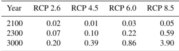
Table 2. Nominal projections (in metres) of AIS contribution to sea level on short-term (2100), medium-term (2300) and long-term (3000) timescales in different RCP scenarios.
Year RCP 2.6 RCP 4.5 RCP 6.0 RCP 8.5 2100 0.02 0.01 0.03 0.05 2300 0.07 0.10 0.22 0.59 3000 0.20 0.39 0.86 3.90
3.1 Nominal projections
We first present nominal projections obtained using the nom-inal values of the parameters given in Table 1. We first present results under nominal conditions in order to assess subsequently the impact of uncertainties on AIS sea-level rise projections. Under nominal conditions, we find (Ta-ble 2) in RCP 2.6 an AIS contribution to sea level of 0.02 m by 2100, 0.07 m by 2300 and 0.20 m by 3000 and in RCP 8.5 an AIS contribution to sea level of 0.05 m by 2100, 0.59 m by 2300 and 3.90 m by 3000. In Fig. 3a, we represented the nominal projections as a function of time in all RCP scenar-ios. We find that the nominal AIS contribution to sea level is rather small in the first decades and starts to increase more significantly around 2100 with a rather constant growth rate. In Fig. 3b–e, we represented the nominal grounded ice re-gion by 3000 for all RCP scenarios. We find that there is little ungrounding by 3000 in RCP 2.6 and RCP 4.5, while we observe a more significant ungrounding in Siple Coast and the Ronne basin in RCP 6.0 and a much more significant ungrounding in Siple Coast and the Amundsen Sea sector in RCP 8.5.
3.2 Parameters-to-projection relationship
One of the advantages of a polynomial chaos expansion is that it provides an explicit approximation to the parameters-to-projection relationship, which can be visualised to gain insight into the relationship between the parameters and the projections.
In Figs. 4 and 5, we used the PC expansions to visualise how the projections depend on each parameter individually (one-at-a-time) while keeping the other parameters fixed at their nominal value under the weakly non-linear sliding law in RCP 2.6 and RCP 8.5, respectively.
Figure 4a–c show that in RCP 2.6 1GMSL increases with an increase in the calving factor non-linearly. The slope is steeper for small values of this parameter, thus suggesting that 1GMSL is more sensitive to small changes about small values than about higher values. Figure 4d–f indicate that 1GMSL increases rather linearly with an increase in the melt factor. Figure 4g–i indicate a rather quadratic dependence on the shelf anisotropy factor for short-term and medium-term projections, with small and large values of this factor leading to more significant ice loss than the nominal value.
Figure 3. (a) Nominal AIS contribution to sea level. Grounded ice (grey area) and ice shelves (light blue area) by 3000 in (b) RCP 2.6, (c) RCP 4.5, (d) RCP 6.0 and (e) RCP 8.5 for the nominal values of the parameters. The present-day grounding line is shown in black.
This quadratic dependence can be explained by the influ-ence of Eshelf on two competing processes: a higher value
of Eshelfsoftens the ice, thus leading to faster ice flow in the
ice shelves, but a higher value of Eshelfalso leads to ice-shelf
thinning, thus reducing ice flux at the grounding line. In addi-tion, we find that 1GMSL depends only little on the bedrock relaxation times (Fig. 4j–o). In fact, lower bedrock relaxation times do tend to stabilise the ice sheet and lower sea-level rise, but this impact is weak compared to the influence of the other parameters. This result may be explained by our orders of magnitude of the bedrock relaxation times being of the order of a few millennia, thus preventing any significant up-lift in the next few centuries. Yet, a recent study by Barletta et al. (2018) has suggested a bedrock relaxation timescale of the order of decades to a century in the Amundsen Sea sector, thus making glacial isostatic adjustment significant in the next decades and centuries in this region. To assess the in-fluence of shorter relaxation times, we performed additional
numerical experiments, albeit not reported in this paper, with a relaxation time for the whole West Antarctic ice sheet that varies widely from a few decades to a few millennia. For this range of values, we found that bedrock relaxation has a more significant influence on the AIS response, with a con-tribution to the uncertainty in 1GMSL that can reach 10 % in RCP 2.6 when τw is allowed to vary widely between 50
and 3500 years.
We find in RCP 8.5 similar trends. However, whereas Fcalv, Fmeltand Eshelfinfluence 1GMSL equally in RCP 2.6,
the melt factor influences 1GMSL most significantly in RCP 8.5. Whereas Fig. 5d–e show that 1GMSL increases rather linearly with an increase in the melt factor, Fig. 5f shows that 1GMSL rather levels off at a plateau for large values of Fmeltfor long-term projections in RCP 8.5.
Additionally, Fig. S2 shows the emulators for several pairs of parameters with the other parameters fixed at their nomi-nal values in RCP 2.6 and RCP 8.5. These figures show es-sentially the same trends as those identified in Figs. 4 and 5, in addition to interaction effects between the parameters. In particular, we find that smaller values of the calving and melt factors lead to mass gain (Fig. S2c), while larger values of the shelf anisotropy and melt factors lead to an important mass loss (Fig. S2d).
3.3 Sea-level rise projections
Under parametric uncertainties, we find (Table 3, Fig. 6) in RCP 2.6 a median AIS contribution to sea level that ranges from 0.02 to 0.03 m by 2100, from 0.07 to 0.13 m by 2300 and from 0.18 to 0.30 m by 3000 for the three sliding laws, as compared with the nominal projections of 0.02 m by 2100, 0.07 m by 2300 and 0.20 m by 3000; and we find in RCP 8.5 a median AIS contribution to sea level that ranges from 0.09 to 0.11 m by 2100, from 0.78 to 1.15 m by 2300 and from 3.18 to 6.12 m by 3000, as compared with the nominal projec-tion of 0.05 m by 2100, 0.59 m by 2300 and 3.90 m by 3000. The median AIS sea-level rise projections are higher than the nominal projections, except for certain cases under the viscous sliding law. The nominal projections are not equal to the median projections because the ice-sheet model exhibits non-linearities, as illustrated in Figs. 4 and 5, and the prob-ability density functions for the parameters are not symmet-ric about their nominal value. As in the nominal projections, we find that in all RCP scenarios and under all sliding laws, the median AIS contribution to sea level is rather small in the first decades and starts to increase around 2100. As in the nominal projections, the median AIS contribution to sea level shows a rather constant growth rate in RCP 2.6, RCP 4.5 and RCP 6.0; contrary to the nominal projection, the median AIS contribution to sea level exhibits initially an acceleration be-fore subsequently exhibiting a deceleration in RCP 8.5 under both non-linear sliding laws (Fig. 6). This behaviour in the median projections in RCP 8.5 is a consequence of the initial rapid collapse of the West Antarctic ice sheet, which
con-Figure 4. Representation of the parameters-to-projection relationships in RCP 2.6 under the weakly non-linear sliding law as given by a PC expansion. The PC expansion is shown for each parameter individually, with the other parameters fixed at their nominal value. PC expansions at (a, d, g, j, m) 2100, (b, e, h, k, n) 2300 and (c, f, i, l, o) 3000.
tributes 3–3.5 m to sea level, followed by a slower retreat in the East Antarctic ice sheet. By contrast, the nominal pro-jections, which involve a melt factor of 0.3, indicate that the West Antarctic ice sheet does not completely collapse by the year 3000.
In RCP 2.6, we find (Table 3) 5 %–95 % probability in-tervals for sea-level rise projections that range from −0.06 to 0.10 m by 2100, from −0.14 to 0.31 m by 2300 and from −0.36 to 0.91 m by 3000. In RCP 8.5, these probability
in-tervals range from −0.03 to 0.23 m by 2100, 0.17 to 2.01 m by 2300 and 0.82 to 7.68 m by 3000. The nominal projec-tions are inside the 5 %–95 % probability intervals. We see that the 5 %–95 % probability intervals indicate an increase in sea level, though a decrease cannot be ruled out for the vis-cous sliding law and cooler atmospheric conditions. Figure 6 highlights that the 33 %–66 % probability intervals become wider under warmer atmospheric conditions and, to a lesser extent, more non-linear sliding conditions. The uncertainty
Figure 5. Same as Fig. 4 but in RCP 8.5.
in the projections due to parametric uncertainty is rather sig-nificant, with possible overlaps between the 5 %–95 % prob-ability intervals for different RCP scenarios. For instance, Fig. 4i shows that a contribution to sea level of about 0.7 m can be reached by 3000 in RCP 2.6 for the extreme value Eshelf=1, while Fig. 5f shows that this value is reached in
RCP 8.5 for very limited sub-shelf melting (Fmelt of about
0.12). This suggests that projections with similar contribu-tions to sea level can arise in different RCP scenarios with different combinations of parameter values. Measuring the
relative dispersion in 1GMSL via the coefficients of vari-ation, that is, the ratio between the standard deviation and the mean value, we find a coefficient of variation of 0.74 in RCP 2.6, 0.67 in RCP 4.5, 0.59 in RCP 6.0 and 0.33 in RCP 8.5 by 3000 under the weakly non-linear sliding law. This demonstrates that the relative uncertainty in 1GSLM pro-jections is higher in cooler RCP scenarios. This results from a much larger increase in the values of 1GSLM projections compared to the increase in their dispersion when the RCP scenario gets warmer.
Figure 6. AIS contribution to sea level. (a) Viscous sliding law, (b) weakly non-linear sliding law and (c) strongly non-linear sliding law. Solid lines are the median projections and the shaded areas are the 33 %–66 % probability intervals that represent the parametric uncertainty in the model.
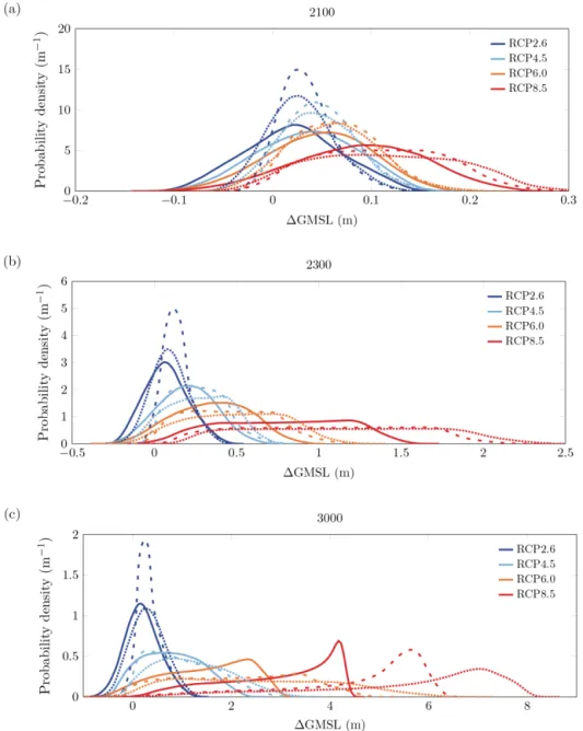
Figure 7 shows the probability density functions for the change in GMSL at different timescales. The results dis-play essentially unimodal probability density functions with wider tails for warmer scenarios and longer timescales. In RCP 2.6, the probability density functions resemble Gaus-sian probability density functions. In RCP 8.5 and at the short and medium timescales, the probability density func-tions are rather flat, which can be explained by the depen-dence of 1GMSL on Fmelt being rather linear (Fig. 5d and
e). In RCP 8.5 and at the long timescale, the probability den-sity functions exhibit a more localised mode at higher values of 1GMSL, which can be explained by the collapse of the
West Antarctic ice sheet and thus the presence of the plateau for higher values of the melt factor (Fig. 5f).
Figure 8 gives the probability of exceeding the threshold values of 0.5, 1.0 and 1.5 m as a function of time. We find that the probability of exceeding 0.5 m by 2100 is negligible (probability of less than 1 %) in all RCP scenarios and under all sliding conditions. In RCP 2.6, the AIS contribution to sea level in the next centuries is strongly limited, with a proba-bility of exceeding 0.5 m by 3000 reaching at most 30 %. In RCP 4.5 and RCP 6.0, we found nominal sea-level rise pro-jections well below 1.5 m, while in RCP 8.5 this threshold is exceeded. In the presence of uncertainties, we find that the probability of exceeding 1.5 m of sea-level rise by 3000
Figure 7. Probability density functions for the AIS contribution to sea level at (a) 2100, (b) 2300 and (c) 3000 under the viscous sliding law (solid lines), the weakly non-linear sliding law (dashed lines) and the strongly non-linear sliding law (dotted lines).
can reach about 35 % in RCP 4.5, about 70 % in RCP 6.0 and about 95 % in RCP 8.5. The last result can be seen from Fig. 5, which indicates that 1GMSL is below 1.5 m only in a small region of the parameter space associated with small values of the melt factor. Furthermore, the shape of the ex-ceedance curves in Fig. 8 provides some insight into the un-certainty in the time when a certain threshold value is ex-ceeded. The time when 1GMSL exceeds 0.5 m with a prob-ability of 33 % under the weakly non-linear sliding law is 2415 in RCP 4.5, 2270 in RCP 6.0 and 2185 in RCP 8.5, while this value is exceeded with a probability of 66 % at 2790 in RCP 4.5, 2430 in RCP 6.0 and 2245 in RCP 8.5. We find that nominal projections overestimate the time when 1GMSL exceeds 0.5 m, with the exceedance time being
be-yond 3000 in RCP 4.5, around 2620 in RCP 6.0 and around 2280 in RCP 8.5.
3.4 Stochastic sensitivity analysis
Figure 9 provides the Sobol sensitivity indices for the change in GMSL on short-term, medium-term and long-term timescales in different RCP scenarios and under different sliding laws. We find that in RCP 2.6, the largest contribu-tion to the uncertainty in 1GMSL stems from the uncer-tainty in the ice-shelf rheology (Sobol indices ranging from 40 % to 60 %) followed by the uncertainty in the calving rate (Sobol indices ranging from 20 % to 40 %) and sub-shelf melting (Sobol indices ranging from 5 % to 25 %). Indeed, in
Figure 8. Probability of exceeding some characteristic threshold sea-level rise values as a function of time, evaluated from the complementary cumulative distribution functions of the probability density functions for 1GMSL. Probability of exceedance under (a) the viscous sliding law, (b) the weakly non-linear sliding law and (c) the strongly non-linear sliding law. Solid lines correspond to a threshold value of 0.5 m, dashed lines to a threshold value of 1 m and dotted lines to a threshold value of 1.5 m.
RCP 2.6, sub-shelf melting plays only a limited role because ocean conditions remain essentially unchanged. Therefore, in RCP 2.6, the dispersion in 1GMSL is mainly controlled by the ice-shelf rheology, which controls ice flow and but-tressing in ice shelves, as well as calving, which reduces the extent of ice shelves and their buttressing.
By contrast, in warmer RCP scenarios and for longer timescales, the dominant source of uncertainty becomes the uncertainty in sub-shelf melting, which accounts in RCP 8.5 for more than 90 % of the uncertainty in sea-level rise pro-jections. As shown in Fig. 5, in RCP 8.5 at 3000 1GMSL varies by several metres over the range of values of Fmelt,
while 1GMSL varies only by a few tens of centimetres over the range of values of the other parameters. Hence, the dom-inant influence of the uncertainty in the melting factor is also a consequence of the rather wide uncertainty range that we chose for this parameter.
Finally, we find that, in all RCP scenarios and under all sliding laws, the uncertainty in the bedrock relaxation times for West and East Antarctica has a limited impact (Sobol in-dex smaller than 1 %), which is a direct consequence of the very limited dependence of the projections on the bedrock relaxation times. Moreover, the interactions between the pa-rameters have a negligible impact as the sums of the
individ-Table 3. Probabilistic projections (in metres) of the AIS contribution to sea level on short-term (2100), medium-term (2300) and long-term (3000) timescales in different RCP scenarios and under different sliding conditions with Schoof’s grounding-line parameterisation. 1GMSL projections are the median projections with their 5 %–95 % probability intervals between parentheses.
Year Sliding (m) RCP 2.6 RCP 4.5 RCP 6.0 RCP 8.5 2100 1 0.02 (−0.06, 0.10) 0.04 (−0.05, 0.12) 0.05 (−0.04, 0.13) 0.09 (−0.03, 0.20) 2 0.03 (−0.01, 0.09) 0.05 (0.00, 0.11) 0.06 (0.00, 0.14) 0.11 (0.01, 0.22) 3 0.03 (−0.03, 0.09) 0.04 (−0.02, 0.11) 0.06 (−0.01, 0.14) 0.11 (0.00, 0.23) 2300 1 0.07 (−0.14, 0.31) 0.20 (−0.09, 0.48) 0.36 (−0.04, 0.72) 0.78 (0.17, 1.35) 2 0.13 (0.01, 0.30) 0.26 (0.03, 0.54) 0.45 (0.06, 0.88) 1.04 (0.27, 1.81) 3 0.09 (−0.09, 0.29) 0.28 (−0.03, 0.58) 0.50 (0.02, 0.96) 1.15 (0.31, 2.01) 3000 1 0.18 (−0.36, 0.82) 0.77 (−0.14, 1.82) 1.60 (−0.01, 2.71) 3.18 (0.82, 4.25) 2 0.30 (−0.01, 0.82) 0.93 (0.08, 2.24) 2.16 (0.15, 4.06) 5.08 (1.36, 6.00) 3 0.30 (−0.25, 0.91) 1.15 (0.08, 2.56) 2.50 (0.34, 5.17) 6.12 (1.65, 7.68)
Figure 9. Sobol sensitivity indices for the AIS contribution to sea level in different RCP scenarios and for different values of the sliding exponent m in Weertman’s sliding law. Sobol indices at (a) 2100, (b) 2300 and (c) 3000. The gap between the height of a bar and the unit value represents the interaction index.
ual Sobol indices account almost entirely for the variances of the projections.
3.5 Projections of grounded-ice retreat
Figure 10 provides insight into the regions of Antarctica that are most at risk of ungrounding in different RCP scenarios and at different timescales under the weakly non-linear slid-ing law. Figure 10 was obtained as follows. First, we deter-mined the 100 % confidence region for grounded ice, that is, the region of Antarctica where ice is certain to remain grounded, and we coloured it in grey. Thus, there is no risk that the grounding line will retreat to within the grey re-gion. Then, we determined the 95 % confidence region for grounded ice, that is, the region of Antarctica that remains covered everywhere with grounded ice with a probability of more than 95 %, and we coloured the portion of the 95 % confidence region that extends beyond the 100 % confidence region in dark blue. Thus, there is a low risk of (less than) 5% that the grounding line will retreat to within the dark blue re-gion. We continued this procedure for decreasing values of the confidence level and using different colours as indicated in the legend in Fig. 10.
We find that ice remains grounded in regions above sea level. By contrast, in all RCP scenarios, the risk of unground-ing is highest in marine sectors of West Antarctica with fast-flowing ice streams, especially in Siple Coast, in the Ronne basin, notably Ellsworth Land, and in the Amundsen Sea sec-tor. In warm RCP scenarios and at longer timescales, we also observe a risk of grounding-line retreat in the Wilkes marine basin in East Antarctica, where the grounding line could re-treat between 100 km (with a risk of 95 %) and 500 km (with a risk of 5 %) from its present-day position. The risk of re-treat in Wilkes basin may partially explain the acceleration in sea-level rise that we observed in Fig. 6 in RCP 8.5. The risk of grounding-line retreat in the Antarctic Peninsula is very limited due to the bedrock topography being above sea level, the marine glaciers being small and a high increase in precipitation in this region.
In RCP 2.6, we observe that the grounding line is quite stable over the next millennium, with the 100 % confidence region for grounded ice being almost unchanged from the present-day grounded ice region (the 100 % confidence re-gion for grounded ice by 3000 only differs from the present-day grounded ice region by a few tens of kilometres). In RCP 4.5, ice remains grounded in most of the West Antarctic ice sheet over the next centuries, but our results also suggest a risk of retreat of the grounding line in some sectors of West Antarctica on longer timescales. In RCP 6.0, we find that the West Antarctic ice sheet belongs by 3000 to the 66 % confi-dence region for grounded ice, while in RCP 8.5, it belongs by 3000 only to the 5 % confidence region. This suggests a risk of 33 % that a major collapse of the West Antarctic ice sheet might occur in RCP 6.0 by 3000 and a risk of 95 % that
a major collapse of the West Antarctic ice sheet might occur in RCP 8.5 by 3000.
As compared with the nominal projections of a limited re-treat of the grounding line in West Antarctica in RCP 6.0 by 3000, we find that the impact of the parametric uncertainty is that a complete collapse of the West Antarctic ice sheet may occur with a risk of 33 % in RCP 6.0 by 3000. Moreover, Fig. 3e suggests that a complete disintegration of the West Antarctic ice sheet is underway by 3000 in RCP 8.5, while in Fig. 10l the West Antarctic ice sheet has already collapsed by 3000.
Additionally, we compared the projections under the weakly non-linear sliding law with projections under the other sliding laws, that is, the viscous sliding law (Fig. S7) and the strongly non-linear sliding law (Fig. S8). We find a lower risk of retreat of the grounding line under the viscous sliding law with a slower disintegration of the West Antarc-tic ice sheet compared to the other sliding laws, especially in the drainage basins of Thwaites and Pine Island glaciers, which belong to the 50 % confidence region for grounded ice by 3000 in RCP 8.5, while they belong to the 5 % con-fidence region by 3000 in RCP 8.5 for the other sliding laws. The strongly non-linear sliding law seems to favour a faster and deeper retreat of the grounding line, especially in the marine sectors of East Antarctica and the drainage basins of Thwaites and Pine Island glaciers. However, Figs. 10i and S8i suggest that ungrounding may be less significant in Siple Coast under the strongly non-linear sliding law than the weakly non-linear sliding law. Actually, MISI may oc-cur when driving stresses overcome resistive stresses (Waibel et al., 2018). Driving stresses are primarily determined by the surface slopes, while resistive stresses depend on the basal sliding coefficient and the ice velocity through the sliding exponent. Driving stresses at the grounding line are higher in the Amundsen Sea sector than in Siple Coast due to steeper surface slopes, leading to a greater sensitivity of the ground-ing line in the former region to non-linearity and a more plas-tic response.
3.6 Influence of the parameter probability density function
So far, we have represented the uncertain parameters Fcalv, Fmelt, Eshelf, τe and τw by a uniform distribution
on a fixed support. For instance, the uncertain parameter Fcalv is represented by a uniform distribution with support
[Fcalv,min, Fcalv,max], where Fcalv,min and Fcalv,max are the
minimum and maximum values in Table 1. We now address the influence of the probabilistic characterisation of the para-metric uncertainty on our probabilistic projections by con-trolling the size of these supports. Hence, we represent the uncertain parameters Fcalv, Fmelt, Eshelf, τeand τwby a
fam-ily of uniform probability density functions indexed by a unique scaling factor α ∈ [0, 1] that controls the supports of the uniform probability density functions. For instance, the
Figure 10. Confidence regions for grounded ice under the weakly non-linear sliding law. Confidence regions are shown at (a, d, g, j, m) 2100, (b, e, h, k,n) 2300 and (c, f, i, l,o) 3000. Results under (a–l) the SGL parameterisation and (m–o) the TGL parameterisation.
uncertain parameter Fcalv is represented for a given value
of α by a uniform distribution with support [Fcalv,nom+
α(Fcalv,min−Fcalv,nom), Fcalv,nom+α(Fcalv,max−Fcalv,nom)],
where Fcalv,nom, Fcalv,minand Fcalv,maxare the nominal,
min-imum and maxmin-imum values in Table 1. For the other parame-ters, the supports are defined similarly. The value α = 0 rep-resents the ice-sheet model without parametric uncertainty, that is, the ice-sheet model for the nominal values of the pa-rameters, and the value α = 1 represents the full uncertainty
ranges considered so far. We propagated the uncertainty from the parameters to the sea-level rise projections for different values of the scaling factor, reusing the emulator that we had built for α = 1 over the whole parameter space. Hence, the projections to follow for α = 0 based on this emulator are not exactly equal to the nominal projections determined directly from the ice-sheet model.
For the long-term projections, Fig. 11a–d show the median and the 33 %–66 % and 5 %–95 % probability intervals as a
function of the scaling factor in the different RCP scenarios under the weakly non-linear sliding law and Fig. 11e–h show the probability density functions for the values α = 0.2, 0.6 and 1.0. We find that the median projections increase with an increase in the scaling factor and range in RCP 2.6 from 0.16 to 0.30 m, in RCP 4.5 from 0.37 to 0.93 m, in RCP 6.0 from 1.11 to 2.16 m and in RCP 8.5 from 3.80 to 5.08 m. In addition, the width of the probability intervals increases with increasing uncertainty in the parameters. While the width of the 33 %–66 % probability interval increases rather linearly with the scaling factor and is rather symmetric about the me-dian, the width of the 5 %–95 % probability interval increases more non-linearly with an increase in the scaling factor, as il-lustrated in Fig. 11a in RCP 2.6 and Fig. 11d in RCP 8.5. The probability density functions attribute higher weight to larger values of 1GMSL under increased parametric uncertainty, with increased weight given to larger values of in particular Eshelfin RCP 2.6 (Fig. 4i) and Fmeltin RCP 8.5 (Fig. 5f).
Fig-ure 11a–d show that the sensitivity of the amount of uncer-tainty in the projections (probability intervals) to the amount of uncertainty in the parameters (scaling factor) is higher for warmer scenarios, with an upper bound between RCP 6.0 and RCP 8.5 as a consequence of the collapse of the West Antarctic ice sheet.
3.7 Projections under a more plastic sliding law We ran the same ensemble of simulations under a more plas-tic sliding law (m = 5). Table 4 and Fig. 12 give for the AIS contribution to sea level the median and the 33 %–66 % and 5 %–95 % probability intervals. As compared with less plas-tic sliding laws (m = 1, 2, 3), we find an increase in sea-level rise projections on short-term and medium-term timescales, thus suggesting a more significant and faster response to per-turbations under more plastic sliding conditions. On a long-term timescale, the ice-sheet mass loss can be less important under m = 5 than m = 3, as observed in the median projec-tions by 3000 in RCP 4.5 and RCP 8.5.
We find that overall the AIS contribution to sea level is an increasing function of the sliding exponent, with the dif-ferences between successive exponents getting smaller as mincreases, as already pointed out by Gillet-Chaulet et al. (2016); for instance, we observe a greater difference in the projections between m = 1 and m = 2 than between m = 3 and m = 5. On longer timescales, tipping points and non-linearities associated with MISI may trigger a slightly dif-ferent response of the ice sheet depending on the initial con-ditions, which could explain the smaller ice loss in our results under m = 5 than m = 3.
3.8 TGL parameterisation
We ran the same ensemble of simulations under the weakly non-linear sliding law using, this time, the TGL parameteri-sation instead of the SGL parameteriparameteri-sation. Under the TGL
parameterisation, Table 5 and Fig. 13 give for the AIS contri-bution to sea level the median and the 33 %–66 % and 5 %– 95 % probability intervals. We find an overall increase in sea-level rise projections compared to our results under the SGL parameterisation. This result was expected as the TGL parameterisation has been shown to increase grounding-line sensitivity to environmental changes (Tsai et al., 2015; Pat-tyn, 2017). The probability of exceeding 0.5 m by 2100 is still negligible (probability of less than 1 %) in all RCP sce-narios. However, the probability of exceeding 0.5 and 1 m by 3000 in RCP 2.6 can reach more than 40 % and 10 %, respectively. For other scenarios, the retreat of the Antarc-tic ice sheet is much more pronounced and faster than under the SGL parameterisation, and the probability of exceeding 1.5 m of sea-level rise by 3000 can reach more than 50 % in RCP 4.5, 80 % in RCP 6.0 and 99 % in RCP 8.5.
Figure 10m–o show the confidence regions for grounded ice under the TGL parameterisation in RCP 8.5. As also pointed out by Pattyn (2017), the TGL parameterisation leads to a faster and more significant grounding-line retreat in the marine sectors and an additional mass loss from East Antarc-tica, especially in the Aurora basin.
4 Discussion
4.1 Comparison of the sea-level rise projections with previous work
Regarding the short-term AIS contribution to sea level, we projected in the RCP 2.6 scenario a median of 0.02–0.03 m under the SGL parameterisation and 5 %–95 % probability intervals from −0.06 to 0.10 m. These projections are simi-lar to other estimates based on other mechanisms. Golledge et al. (2015) reported an AIS contribution to sea level be-tween −0.01 and 0.10 m with the lower and higher bounds corresponding to the absence and presence of sub-grid inter-polation of basal melting at the grounding line. DeConto and Pollard (2016) reported an AIS contribution to sea level be-tween −0.11 and 0.15 m based on a model calibration with a range of Pliocene sea-level targets between 5 and 15 m higher than today. In the same scenario, we found an in-creased AIS response under the TGL parameterisation with a median AIS contribution to sea level of 0.06 m and a 5 %– 95 % probability interval between 0.00 and 0.14 m by 2100. These higher projections are similar to the higher projections (0–0.22 m) reported by DeConto and Pollard (2016) for a higher range of Pliocene sea-level targets between 10 and 20 m. In all RCP scenarios, under all sliding laws and under both grounding-line parameterisations, our results suggested that the AIS contribution to sea level does not exceed 0.5 m by 2100, with a probability of at least 99 %. These results are in agreement with Ritz et al. (2015), who determined an AIS contribution to sea level that lies between 0.05 and 0.30 m, and Golledge et al. (2015), who found an AIS contribution to