Contents lists available atScienceDirect
Energy Conversion and Management
journal homepage:www.elsevier.com/locate/enconmanTechnical and economic optimization of subcritical, wet expansion and
transcritical Organic Rankine Cycle (ORC) systems coupled with a biogas
power plant
Olivier Dumont
a,⁎, Rémi Dickes
a, Mattia De Rosa
b, Roy Douglas
c, Vincent Lemort
a aEnergy System Research Unit, Aerospace and Mechanical Engineering Department, University of Liège, Allée de la Découverte 17, B4000 Liège, Belgium bSchool of Mechanical & Materials Engineering, University College Dublin, Belfield, Dublin 4, IrelandcSchool of Mechanical & Aerospace Engineering, Queen's University Belfast, Ashby Building, Stranmillis Road, Belfast, United Kingdom
A R T I C L E I N F O
Keywords: Biogas power plant Waste heat recovery Organic Rankine cycle Thermo-economic optimization Subcritical
Trans-critical Wet expansion
A B S T R A C T
Generally, > 40% of the useful energy (cooling engine and exhaust gases) are wasted by a biogas power plant through the cooling radiator and the exhaust gases. An efficient way to convert this waste heat into work and eventually electricity is the use of an organic Rankine cycle (ORC) power system. Over the last few years, different architectures have been widely investigated (subcritical, wet expansion and trans-critical). Despite the promising performances, realistic economic and technical constraints, also related to the application, are re-quired for a meaningful comparison between ORC technologies and architectures. Starting from the limited literature available, the aim of the present paper is to provide a methodology to compare sub-critical, trans-critical and wet expansion cycles and different types of expanders (both volumetric and turbomachinery) from both technical and economic point of view, which represent one of the main novel aspects of the present work. In particular, the paper focuses on the thermo-economic optimization of an ORC waste heat recovery unit for a 500 kWe biogas power plant located in a detailed regional market, which was not investigated yet. By means of a genetic algorithm, the adopted methodology optimizes a given economic criteria (Pay-Back Period, Net Present Value, Profitability Index and Internal Rate of Return) while respecting technical constraints (expander lim-itations) and thermodynamic constraints (positive pinch points in heat exchangers, etc.).
The results show that optimal ORC solutions with a potential of energy savings up to 600 MWh a year and with a pay-back period lower than 3 years are achievable in the regional market analysed.
1. Introduction
Nowadays, the increase of energy consumption has led to concerns due to the strong environmental impact in terms of global warming and pollution. The EU emanated several directives aimed to reduce the environmental impact of our society by fostering the development of advanced and effective energy efficiency policies[1].
In this context, recovering and reusing the low-grade heat wasted by industrial processes represents an effective way to increase the overall performance of a process and, consequently to reduce the primary en-ergy consumption and the carbon footprint. Generally, the so-called Waste Heat Recovery (WHR) can be applied to any process where a heat source with a temperature higher than 80–100 °C occurs[2].
Among others, the Organic Rankine Cycle (ORC) technology is a promising technique to produce electricity by exploiting this low-grade heat. Like a conventional steam power plant, an ORC cycle is a Rankine
cycle in which an organic substance (usually synthetic refrigerants or hydrocarbons) is adopted as working fluid. A strong interest on this technology has been raised over the last few years due to the wide range of possible applications. As for instance, Campana et al.[3] es-timated an installation potential of 2705 MWein Europe, which would
lead to about 21.6 TWheof electricity production with a corresponding
reduction of greenhouse gas emissions (GHG) of about 8.1 million. Consequently, a lot of efforts have been put by researchers and en-gineers to investigate deeply the performance and benefits of this technology[4–8].
Generally, the investment cost of an ORC system is in the 1200–9500 USD/kWe range, but, as highlighted by[9–10], the specific application, the type of heat sources available and the ORC architecture strongly influence the actual values. Moreover, the specific market context and the investment policy adopted assume a relevant role when a potential investment is assessed [11]. Notwithstanding, a lack of
https://doi.org/10.1016/j.enconman.2017.12.022
Received 26 August 2017; Received in revised form 6 December 2017; Accepted 7 December 2017
⁎Corresponding author.
E-mail address:[email protected](O. Dumont).
0196-8904/ © 2017 Elsevier Ltd. All rights reserved.
information is still present from an economic point of view taking into characteristics of the market in which the system is located in, and it represents a paramount aspect for the diffusion of this technology.
One of the most promising applications for ORC systems is re-presented by biogas power plants [12–15]. Generally, biogas is pro-duced locally by the anaerobic digestion (AD) of organic substrates coming from organic waste streams, e.g. biological feedstocks from agricultural sectors [13], and it can be used as renewable fuel for transports (after a cleaning treatment) or to produce electricity by means of CHP engines (biogas power plants, or AD-CHP)[14]. As for other biofuels, biogas is an important priority of the European energy policy since it is a cheap and CO2-neutral source of renewable energy,
which offers the possibility of treating and recycling a wide range of agricultural residues and products. Therefore, an impressive develop-ment of AD-CHP plants occurred over the last few years and > 17,000 plants were operational in Europe in 2014 with a total installed capa-city of 8.293 GWel [15]. Generally, only 40% of the biogas energy
content is transformed into electricity[16], while about 25% is used for the internal parasitic load and for heating the digester to keep the biological temperature required to allow the chemical processes. The remaining part is generally released into the atmosphere in form of heat by the exhaust gas (high temperature, > 350 °C) and by the radiators (low temperature, < 120 °C). An organic Rankine cycle system might be used to exploit part of this heat to produce further electricity,
increasing the overall performance of the AD-CHP system.
Despite the amount of work done to analyse the ORC systems, in-cluding the direct use of biogas as thermal source of the ORC system [13,16,17–20], the WHR application for biogas plant has not been fully investigated yet. As for instance, Yangli et al.[14]performed a tech-nical investigation of subcritical and supercritical ORC systems which exploit the heat rejected from a biogas CHP engine, obtaining ORC thermal efficiencies of 15.51% and 15.93% for subcritical and super-critical cycles respectively. The authors concluded their work high-lighting that a thermo-economic analysis should be carried out to detect the configuration which guarantees the best repayment period. At this regard, Sung et al.[15]performed a thermo-economic analysis of a biogas micro-turbine system coupled with a subcritical ORC cycle with a turbine as expander. The analysis, limited to one workingfluid (n-Pentane), is mainly focused on partial load operating conditions of the biogas micro-turbine. Notwithstanding, the authors demonstrated that the introduction of a bottoming ORC provides a net gain from an nomic point of view, despite the analysis was limited to only one eco-nomic parameter (Net Present Value, see Section3.3).
Therefore, a lack of thermo-economic analyses on WHR-ORC for biogas power plant applications is still present. In this context, the aim of the present paper is to extend the analysis to a wider range of po-tential ORC configurations (namely subcritical, trans-critical and wet expansion cycles [8,21–22]) and working fluids. Different AD-ORC Nomenclature A area [m2] AD anaerobic digester B capacity parameter [W] or [m2] Bo boiling number [–] C cost [€]
Cp isobaric specific heat [J/kg/K]
CHP combined heat and power CF cashflow [€]
D correlation coefficient [–] Dh hydraulic diameter [m]
E exergy [kJ/kg] f friction factor
F factor [–]
h convective heat transfer coefficient [kW/(m2K)] H enthalpy [kJ/(kg)]
i index
Inv investments [€]
IRR interest rate of return [–]
j index
k thermal conductivity [W/mK] K correlation coefficient [–] L characteristic length [m] LCOE levelized cost of electricity LHV low heating value [J/kg]
ṁ massflow rate [kg/s] NI Northern Ireland NPV net present value [€] Nu Nusselt number ORC organic Rankine cycle p pressure [bar]
P pitch [m]
PBP pay back period [–] PEF primary energy factor [–] PI profitability index [–] Pr Prandtl [–]
Q̇ heat transfer rate [W] r discount rate [–]
R thermal resistance [K/W] Re Reynolds [–]
SP size parameter [–] T temperature [°C]
U heat transfer coefficient [W/(m2·K) V̇ volumetricflow rate [m3/s] VC volume coefficient [m3/J]
VR volume ratio [–]
W energy [kWh]
WHR waste heat recovery
Ẇ power [W]
x state of thefluid at the exhaust of the evaporator y time [year] Greek β Chevron angle [°] Δ difference ε effectiveness [–] η efficiency [–] μ dynamic viscosity [kg/m/s] Indices aux auxiliary b bulk el electrical eV evaporator ex exhaust exp expander gas gas is isentropic
LMTD log mean temperature difference
net net pp pump sf secondaryfluid su supply w wall wf workingfluid
configurations have been analysed and both volumetric and rotational expanders have been compared for each case study, taking into account their intrinsic constraints. The economic performance of the invest-ments has been investigated considering a specific market context and introducing several economic indexes – mainly Net Present Value (NPV), Pay Back Period (PBP), Profitability Index (PI) and Internal Rate of Return (IRR)[11].
2. Waste heat recovery for biogas power plant through an ORC power system
2.1. Organic Rankine cycle power system technology
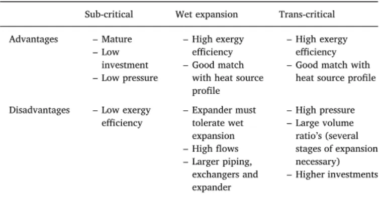
ORC power systems have been used to generate electricity from waste heat for several decades[23]. Apart from the standard sub-cri-tical ORC architecture, other configurations have been investigated, such as wet expansion[21,24–25]and trans-critical cycles[26](Fig. 1). Superheating, quality and specific approach are three parameters that are useful to define the thermodynamic state of the fluid at the inlet. Table 1summaries the advantages and disadvantages for each archi-tecture of ORC power system.
Generally, wet expansion and trans-critical cycles present higher energy and exergy efficiencies than the standard sub-critical ORC, due to the better matching of the temperature profiles in the evaporator, as demonstrated in [7]. However, wet expansion cycles has high mass flows for a given installed power (greater piping dimension) and it requires an expander able to handle two-phase flows, leading to lim-itations in the expander choice and affecting the overall performance. On the other hand, the trans-critical cycle requires higher pressures than the wet expansion and sub-critical cycles. Although more efficient, it leads to higher costs for the evaporator and the expander.
In order to understand the economic suitability of a system for a specific application, it is necessary to perform a full thermo-economic analysis[14]. Thermo-economic or techno-economic optimization ap-proaches comparing different ORC architectures are rather scarce in the scientific literature[26–28]. Lecompte et al.[29]performed a thermo-economic optimization between the three architectures, while ac-counting for practical constraints related to the expansion device. This paper shows the interest of the wet expansion cycle but no evaluation of performance of both a turbine and a volumetric expander is carried out. Furthermore, the evaporator super-heating for the subcritical ORC and the trans-critical pressure are not optimized and are assumed constant. One of the main novelty of this paper is that these two parameters are free to vary and are optimized to achieve the best system performance according with the objective function chosen.
In summary, the challenge is to devise an ORC design strategy flexible enough to compare different cycle architectures and expander technologies (volumetric and turbines) based on thermo-economic criteria. This paperfills up this gap and applies this methodology to an ORC system coupled with a biogas power plant.
2.2. Anaerobic digester applications
Over the last few decades, a strong development of AD biogas power plant occurred in Europe: about 17,240 biogas plants have been in-stalled[19]with a total installed capacity of 8.3 GWel. Generally, an
AD-CHP system uses the biogas produced by the AD system (typically several tanks where the biological reactions occur) as a fuel for a biogas engine to produce electricity and thermal energy. A lot of con figura-tions has been developed and built; since the focus of this paper is on ORC applications, the complete technical description of AD-CHP sys-tems is demanded to[18–20].
On the other hand, AD-CHP sector represents a promising applica-tion for ORC system since about 29% of the thermal heat available (high/medium grade) is currently wasted. This heat might be recovered and reused by an ORC system for electricity production, increasing the overall performance of the system. ORC systems coupled with AD-CHP may have a potential output between 5000 and 7000 GWhe/year only in Europe.
2.2.1. Local market context
The local biogas power plant market in Northern Ireland (NI) has been used in this paper to assess the economic suitability of ORC sys-tems for AD-CHP plants. Generally, Ireland is characterised by a great potential in terms of biogas production, mainly thanks to the high contribution of agriculture (e.g. about 10,000 km2of land in NI are devoted to agricultural activities). Only in Northern Ireland, the ex-ploitation of the organic resources available (estimated to be between 207 and 500 thousands of tons, including municipal, commercial and industrial wastes) might bring to a potential coverage between 5% and 23% of the total electric energy demand[30,31]. Thanks to this positive background (and to the incentives put in place to support the AD in-dustry), the number of AD plants has grown exponentially over the last few years, as shown inFig. 2.Table 2reports the current (April 2016) and potential AD installations in Northern Ireland.
Fig. 1. T-s diagram for sub-critical cycle (a), wet expansion cycle (b) and trans-critical cycle (c). Table 1
Advantages and disadvantages for each architecture of ORC power system.
Sub-critical Wet expansion Trans-critical
Advantages – Mature – Low investment – Low pressure – High exergy efficiency – Good match
with heat source profile
– High exergy efficiency – Good match with
heat source profile Disadvantages – Low exergy
efficiency – Expander must tolerate wet expansion – High flows – Larger piping, exchangers and expander – High pressure – Large volume ratio’s (several stages of expansion necessary) – Higher investments
In order to investigate the economic suitability of the ORC tech-nology in the AD-CHP sector, a medium size typical AD plant in Northern Ireland was used as Ref. [31–33]. The plant has a nominal installed power of 500 kWe with a conversion efficiency of 42% (Eq. (1)) and a feedstock consumption of 16,000 tons/year (see Section3.5).
= η W m LHV ̇ ( ̇ · ) el biogas (1)
The income from the electricity produced by the AD consists of two components: (i) the selling electricity price, which is generally afixed feed-in tariff typically guaranteed for 20 years and, (ii) the Northern Ireland renewable energy subsidies, which generally depend on the size of the plant[34]. In the present work, the feed-in tariff is assumed equal to€27.1/MWh: €5.42/MWh for the basic feed-in tariff, €10.73/MWh from the Renewable Obligation Certificates and 10.39€/MWh which is added to the feed-in tariff to promote AD power plants. Finally, trends of electricity prices and inflation rates have been considered in ac-cordance with[35].
3. Methodology 3.1. Thermodynamic model
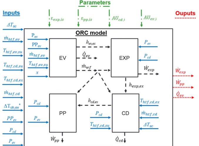
A steady-state model of a non-regenerative ORC (Fig. 3) has been developed in Matlab®. The thermo-physical properties of the fluids are retrieved from CoolProp[36]and the model is used to determine the optimal cycle (subcritical, wet expansion and trans-critical) over a wide range of conditions.
The approach and the main assumptions are described in the fol-lowing sections.
3.1.1. Workingfluid
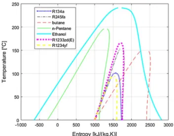
The working fluids considered in this paper are R134a, R245fa, Butane, n-Pentane, Ethanol, R1233zd(E) and R1234yf, which are standardfluids for ORC power systems[37,38]. Fig. 4presents their respective T-s diagrams. For each fluid, the maximum degradation temperature (thermal stability) is imposed as a constraint to limit the temperature at the exhaust of the evaporator.
The comparison between different refrigerants, which represents an added value of the present study, is paramount for a correct system Fig. 2. Operative biogas power plants in Northern Ireland[33].
Table 2
Biogas production in Northern Ireland[30–33]
Units Value
AD Plants (operating/planned) – 42/86 Total installed capacity (2016) MWe 23.99 Feedstock demand (2016) tpa/y 479,950 Biogas production capacity (2016) Nm3 31.74 (millions)
Potential biogas capacity Nm3 133–585 (millions)
Potential electric energy capacity GWhel/y 458–2020
Potential heat energy capacity GWht/y 655–2885
design and optimization and, therefore, future work will be aimed to extend the range offluids analysed. Moreover, it is important to state that other criteria, such as safety (flammability, toxicity, availability, etc.), are not directly considered in this thermo-economic study for the sake of simplicity, but they should be taken into account at thefinal stage.
3.1.2. Expanders
One of the main novelty of this paper compared to the literature (e.g.[4]) is that two different expander technologies are investigated: the turbine and the screw expander. Among the volumetric expanders, only the screw expander case is investigated because of the lack of available data on the cost of other technologies[39].
The isentropic efficiency of the expander, defined according to Eq. (2), is supposed to be constant and equal to 75% for both turbine and screw expanders. This hypothesis is assumed valid since it is in line with what reported in the literature[4,7,40,41].
= − ε W m h h ̇ ̇ ( ) exp is exp el exp su exp ex is , , , , , (2)
Some practical constraints have been implemented to make sure the expander works with this efficiency:
•
Turbine: the size parameter (SP, Eq.(3))– a paramount value pre-dicting the efficiency penalties related to flow compressibility and/ or small blade dimensions– must be between 0.2 m and 1 m, while the volume ratio (VR, Eq.(4)) must be lower than 50[42]. Since a turbine presents difficulties to handle wet expansion, the ORC model imposes a minimum superheating of 1 K during the whole expan-sion. = SP V H ̇ Δ exp in is , 1/2 1/4 (3) = VR V V exp ex exp in , , (4)•
Volumetric expanders (i.e. screw): the Volume Coefficient (VC, Eq. (5)) defines the ratio of the outlet volumetric flow divided with the output power. It is constrained between 0.25 and 0.6 m3/MJ[7].Moreover, the volume ratio (Eq.(4)) is limited to 5 for one screw expander[43]. When the volume ratio is higher than 5, the ORC model allows the connection of multiple screw expanders in series to limit the volume ratio of each machine to a maximum of 5.
= VC V W ̇ ̇ exp ex exp , (5) 3.1.3. Pump
The efficiency of the pump is calculated as shown in Eq.(6). In order to avoid cavitation, a sub-cooling of 5 K is set[44].
= − ε m H H W ̇ ( ) ̇ pp pp ex pp su pp el , , , (6) 3.1.4. Heat exchangers
The heat exchangers are modelled considering the global thermal conductance of a given zone of a heat exchanger (AU), calculated by combining the thermal resistances of the secondary fluid (sf), the workingfluid (wf) and the inner wall (Eq.(7)).
⎜ ⎟ = ⎛ ⎝ + + ⎞ ⎠ − AU A h A h R 1 1 sf sf wf wf wall 1 (7) Considering that the aim of the present work is to investigate the system performance in a preliminary stage of the design, when detailed information (e.g. geometrical constraints) are not available, several simplifications and assumptions are required. Firstly, the wall thermal resistance is assumed to be negligible, due to the high conductivity of the common materials used in ORC heat exchangers[44]. Therefore, only the workingfluid and secondary fluid convective heat transfer coefficients h are computed by means of correlation based on the Nusselt number.
=
h Nuk
L (8)
Regarding the single-phase turbulentflow, the Gnielinsky equation [45]can be used to calculate Nu, as shown in Eq.(9):
= − + − ⎛ ⎝ ⩽ ⩽ < < ⎞ ⎠ Nu f Re Pr f Pr Pr Re ( /8)·( 1000) 1 12.7( /8) ( 1) 0.5 2000 3·10 5·10 0.5 2/3 3 6 (9)
where Re and Pr are the Reynolds and Prandtl numbers respectively, while f is the friction factor, which can be calculated using the Petukov equation[46].
Boiling and condensation may occur on the refrigerant side de-pending on the type of ORC cycle analysed. Eqs.(10) and (11)show the Nusselt correlations for two phases processes, i.e. evaporation (Eq. (10)) and condensation (Eq.(11))[47–48]:
= ⎛ ⎝ − ⎞⎠ ⎜ ⎟ − − ⎛ ⎝ − ⎞ ⎠ −
(
)
Nu P D π β Re Bo Pr 2.8 2 h P D π β 0.04 2.83 0.74 2 0.3 0.4 h 0.082 0.61 (10) = ⎛ ⎝ − ⎞⎠ ⎜ ⎟ − − ⎛ ⎝ − ⎞ ⎠ −(
)
Nu P D π β Re Pr 11.2 2 h P D π β 2.83 4.5 0.74 2 1/3 h 0.23 1.48 (11) whereβ is the chevron angle, Re the Reynolds number, Pr the Prandtl number, Dhis the hydraulic diameter, Bo is the boiling number, P is thepitch,μ is the dynamic viscosity, k is the thermal conductivity, Cp is the specific heat.
The heat transfer in supercritical conditions is affected by several phenomena, in particular when the pseudo-critical temperature (i.e. the temperature where the maximum of the specific heat occurs) is crossed [49]. The strong variation of the properties in this region may lead to several effects related to the fluid acceleration, high specific heat layer, buoyancy (for vertical channels), etc., which can deteriorate or enhance locally/globally the heat transfer [49]. In order to reproduce these phenomena, several authors introduced correction factors in the Nusselt correlation[50–52].
Despite the wide utilisation of the above equations, most of them are only partially validated (range offlow, geometry, etc.) with only one workingfluid and only valid for a given type of heat exchanger[4]. Fig. 4. T-s diagram for R134a, R245fa, Butane, n-Pentane, Ethanol, R1233zd(E) and
Moreover, they require the knowledge of thefluid conditions at the wall of the pipe, which means that information coming from detailed ana-lyses (i.e. CFD) are required. Furthermore, an accurate modelling re-quires the detailed geometry of the heat exchanger, generally not known during the preliminary stage of the design at which this paper is aimed at.
No other accurate general correlations exist for predicting the heat exchange coefficient of refrigerant in different states (liquid, vapor, evaporation, condensation, trans-critical), as shown in [53]. Con-sidering that the heat transfer coefficient on the working fluid side is much higher than the heat transfer coefficient on the secondary fluid side in most of the applications[54], the workingfluid contribution is neglected in Eq.(7). It is important to state that this assumption can be considered valid only during a preliminary stage of the system design, when the analyses are focused on determining which size of the system must be targeted, depending on the specific objective function chosen. During the subsequent design stage, when the optimisation procedure must get into each component to define their specifications, a detailed analysis is required.
In accordance with the above considerations, typical values[48]of the global heat transfer coefficient in the range of 3000–10,000 W/ (m2K) and 500–2500 W/(m2K) have been obtained for the condenser
and the evaporator respectively. The surface area required by each zone (i) of the heat exchangers is then computed by using the LMTD method for each zone (liquid, two-phase or vapor) (Eq.(12)).
= A Q U T ̇ ( ·Δ ) i i i LMTD (12)
The Logarithmic Mean Temperature Difference ( TΔ LMTD) is eval-uated as shown in Eq.(13), whereΔT1andΔT2are the temperature
differences between the two streams at each side of the heat exchanger.
= −
( )
T T T Δ Δ Δ ln LMTD T T 1 2 Δ Δ 1 2 (13)The difference between the inlet and outlet temperature of the secondaryfluid in the condenser (glide) is set to 10 K, while the cold sink supply temperature is equal to 20 °C. The secondaryfluid in the condenser is water, cooled by air using a cooling tower (Section3.5). 3.1.5. Cycle
The layout of the ORC system is depicted inFig. 3, whileFig. 5 presents the solver architecture of the ORC model.
The net power generation of the ORC is calculated using Eq.(14), where the pump and auxiliary consumptions are considered.
= − −
Ẇnet Ẇexp Ẇpp Wauẋ (14) Then, the energy efficiency is defined by Eq.(15).
= η W Q ̇ ̇ net ev (15)
The model assumptions and the parameter ranges used in the pre-sent work are listed inTable 3. In particular:
– Each process is considered in steady-state regime. Potential and kinetic energies of theflowing fluid are considered negligible. – Pressure drops and heat losses through pipe lines are neglected. – The maximum pressure is limited to 3 times the critical pressure of
the selectedfluid (for the robustness of the algorithm) while the maximum condensation temperature is limited to 100 °C which is the case of the majority of ORC power systems[38].
Fig. 5. Inputs, outputs, parameters and solver architecture of the cycle model. The parameter x represents: (i) the over-heating for sub-critical cycles, (ii) the quality for wet expansion cycles and (iii) approach (Fig. 1) for trans-critical cycles.
– The state of the fluid at the inlet of the expander is defined in dif-ferent ways depending on the cycle architecture:
o Sub-critical cycle: superheating is free to vary between 0 K and 200 K.
o trans-critical cycle: the difference between the expander suction temperature and the hot source supply temperature (approach) is varied between 0 and 200 K.
o wet expansion cycle: the quality of thefluid at the exhaust of the evaporator is free to vary between 0 and 1.
– The minimum condensation pressure is set to 1 bar to avoid the infiltration of air into the system.
The primary energy savings are computed assuming that the whole electricity produced by the ORC power system does not need to be produced by another power plant or imported from the grid. The pri-mary energy factor, ratio between the electrical energy and the re-quired primary energy to produce it (Eq.(16)), is assumed equal to 2 [55]. = PEF W W el primary (16)
The constraints of positive pinch-point and dry expansion of the turbine have to be strictly satisfied. However, to guarantee a con-vergence of the optimiser, the size parameter (SP), the maximum vo-lume ratio (VR) and the vovo-lume coefficient (VC) can be varied outside the range fromTable 3. When one of the variables SP, VC or VR (called z in Eq.(17)) gets a value outside the acceptable range (zlim), the cost of
the expander is multiplied by a factor F (Eq.(17)). Then, it is verified a posteriori that the square term in Eq.(17)leads to an optimal solution within the acceptable range, if a feasible solution exists.
= −
F (zactual zlim)2 (17)
3.2. Exergy analysis
The exergy analysis is a useful tool for the design and the optimi-zation of energy systems since it permits to consider the“quality” of the energy fluxes of the system. The exergy related to a given
thermodynamic state i can be calculated as shown in Eq.(18), where the index 0 indicates the reference state (in this case, saturated liquid of workingfluid at the ambient temperature, i.e. the lowest reachable state in the condenser).
= − − −
Ei m H Ḣ (( i 0) T S S0( i 0)) (18) The exergy balance equation is shown in Eq.(19), where Qjis the
heat transfer rate at temperature Tj,Ẇis the work rate and I represents
the total exergy destroyed due to irreversibilities.
∑
⎜⎛ ⎟∑
∑
⎝ − ⎞ ⎠ − + − − = T T Q W m E m E I 1 ̇ ̇ ̇ · ̇ · 0 j j j x su x su x y ex y ex y 0 , , , , (19) The exergy balance equation is solved for each ORC component and, then, the exergy efficiency is calculated according to Eq.(20).= = − +
η Exergy used Exergy supplied
Exergy destroyed Exergy not used Exergy supplied 1 exergetic (20) 3.3. Economic model 3.3.1. Investment costs
In order to determine the overall investment cost of the ORC system (starting from its thermodynamic parameter), the cost correlation shown in Eq.(21)was used[53]. The parameter B corresponds to the heat transfer area for heat exchangers, while for pumps and turbines it corresponds to the power. The costs of the heat exchangers are also related to their material and the maximal pressure (p). Therefore, a correction factor Fb(to be multiplied with C to get the total cost) is
introduced (Eq.(22)).Fpis computed with Eq.(23), while the values of all the coefficients for each component (Fm, Bi, Di, Ki) can be found in [56].
= + +
C K K B K B
log( ) 1 2log( ) 3(log )2 (21)
= +
Fb B1 B2F Fp m (22)
=D +D p +D p
log(F )p 1 2log( ) 3(log )2 (23)
Table 3
Optimization parameters and model assumptions.
Optimization parameters
Minimum Maximum
Evaporator pressure [bar] Condenser pressure 3 × Pcrit
Condenser pressure [bar] Min(Psat(Tsf,cd,su),1) Psat(100 °C)
Inlet expander Over-heating (Sub-critical) 0 200
Approach (Wet expansion) 0 200
Quality (Trans-critical) 0 1
Evaporator pinch-point [K] 1 200
Fluid (cost, Tdegradation) R134a, R245fa, Butane, Pentane, Toluene R1233zd(E) and R1234yf
Architecture Sub-critical, wet expansion, trans-critical Fixed parameters
Heat sourcefluid mass flow rate [kg/s] [0.05;0.11; 0.18; 0.25; 0.32; 0.38; 0.45; 0.52; 0.59; 0.66; 0.72; 0.79; 0.86; 0.93; 1] Heat source supply temperature [°C] 300
Condenser glide [K] 10
Heat sinkfluid supply temperature [°C] 20
Sub-cooling [K] 5
Expander isentropic efficiency [–] 0.75 Pumps (workingfluid & secondary fluid) isentropic efficiency [–] 0.7
Ambient losses Neglected
Fan of the cooling tower consumption 5% of condenser thermal power Constraints
Turbine Size Parameter (SP) [0.02–1] Volume coefficient (VC) [m3/MJ] [0.25–0.6]
Turbine superheating during expansion [K] > 0 Turbine volume ratio (VR) [–] < 50
Screw volume ratio [–] < 5
The overall cost includes direct costs (installation of equipment, piping, instrumentation and controls), indirect costs (engineering and supervision, transportation), contingency costs and fees, assumed at 15% and 3% respectively. Finally, a cost correlation based on the ex-haust volumeflow is used for the screw expander[28].
Since the coefficient used refers to 2001 prices[56], the inflation rate was introduced to determine the current value.
3.3.2. Economic indicators
Four economic indicators have been considered in this study to compare the economic performance of each ORC architecture:
– The Net Present Value (NPV – Eq. (24)), which is the difference between the cashflow (CF – defined as the income from the elec-tricity sold less the operating cost of the plant), including the dis-count rate (r, assumed equal to 4%), and the investment costs. The considered time (y) is equal to 20 years, which corresponds to the typical lifetime of an ORC power system[26].
∑
= + − = NPV y CF y r inv ( ) ( ) (1 ) i y i 1 (24)– The Internal rate of Return (IRR), which consists of the calculation of the term r in Eq.(24)imposing a NPV equal to zero on a 20 years basis.
– The Pay-Back Period (PBP), which is the time required to recover the investment cost (NPV equal to zero– Eq.(24)). It minimizes the capital risks associated with the investment costs.
– The Profitability Index (PI – Eq.(25)), which determines the ratio between the cashflow, including the interests, and the investment cost. This indicator can be considered as a measure of the invest-ment efficiency, giving an idea about the ratio between money earned and original investment. It can be effectively used to rank different alternatives. As for the NPV, y is taken equal to 20.
∑
= + = PI y inv CF y r ( ) 1 ( ) (1 ) i y i 1 (25)– the Levelized Cost Of Electricity (LCOE), defined according to Eq. (26)where W(i) is the energy generated during the period i. This index is not used as objective function in the present work, but it is calculated for each case analysed.
∑
∑
= = + = + LCOE i y inv i r i y W i r 1 ( ) (1 ) 1 ( ) (1 ) t t (26) It is important to state that the choice of the performance indicator reflects the investment policy of the company/investor and it may have a significant impact on the optimization results, leading to different technical configurations, as demonstrated in[11].3.4. Thermo-economic optimization tool
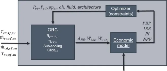
A genetic algorithm is used to solve the thermo-economic optimi-zation (Fig. 6): for the given inputs (heat source and heat sinkflows,
ṁev sf su, , and ṁcd sf su, , , and temperatures Tev sf su, , and Tcd sf su, , ), the ORC model is run using a given configuration of optimization parameters (mainly workingfluid, architecture, evaporator pinch-point, evaporator and condenser pressure and expander inlet conditions). Regarding the genetic algorithm, the tournament size is 4, the number of individuals that are guaranteed to survive to the next generation is 5% of the po-pulation size and the fraction of the next generation, other than elite children, that are produced by crossover is 0.8.
The ORC model computes the electrical production and it gives as outputs: the expander power production (Ẇexp), the heat transfer areas of each exchanger (AHE) and the auxiliary consumption related to
pumps and fans (Ẇaux). Based on these outputs and on the feed-in tariff of electricity, the economic model estimates the investment cost and, then, the economic indexes (NPV, PPB, IRR and PI). Finally, the opti-mizer gives the optimization parameters (Table 3) to the ORC model while respecting the aforementioned constraints (Table 3). The opti-mizer can optimize the PBP, the NPV, the IRR or the PI as set by the user (Section3.1.3).
It is important to state that the optimizer tends to match the T-s profiles of the heat source and the working fluid to reduce the irre-versibilities without achieving a too low evaporator pinch-point (leading to high exchange area and therefore increased costs). An ex-ample is provided inFig. 7where R245fa was used as workingfluid. 3.5. Case studies
The methodology presented in Section3.4 is applied to the case study of an ORC system coupled with a biomass power plant consisting of an AD producing biogas for a CHP engine (Fig. 8).
The plant is assumed working for 7971 h per year at full load. The engine power is 500 kWe with an efficiency of 42% and about 247 kW thermal power is rejected by the exhaust gases at 470 °C and 263 kW by the engine coolant. A maximum of 200 kW is used to heat the digester to ensure an optimal temperature (∼45 °C) for the biological processes, while the remaining is rejected through an air-cooled exchanger. Using the exhaust gases (case study 1) or the sum of the exhaust gases and the engine coolant (case study 2) to feed an ORC power system (Table 4and Fig. 9) is the idea this paper is focused on. The minimum exhaust gases temperature isfixed to 180 °C to avoid condensation phenomena.
Two heating options for the anaerobic digester were detected:
•
part of the waste heat from the engine is used to heat the digester while the remaining heat is used by the ORC (option 1)•
all the waste heat is used by the ORC power unit the heat required by the anaerobic digester is provided by a gas burner (option 2). The costs (i.e. benefit lost) associated to option 1 are equal to the thermal energy necessary for the digester multiplied by the ORC effi-ciency multiplied by the feed-in tariff of electricity. For option 2, the costs (or loss of benefits) associated are equal to the required thermal energy for the AD times the specific cost of gas burnt in the boiler. Therefore, for a given amount of thermal energy required by the anaerobic digester, option 1 is less interesting than option 2, if Eq.(27) is respected.> −
ηORC·Cfeed in el, Cretail gas, (27)
With a gas retail price of€4.87/MWh and a feed-in electricity price of€27.1/MWhe, ORC efficiencies > 18% would be required to make it economically attractive. This very high ORC efficiency cannot be
reached with reasonable investment costs (see Section4). Therefore, covering the thermal demand by exploiting the wasted thermal energy on site is always more convenient than converting it into electricity through an ORC power system.
4. Results
4.1. Cycle architecture and expander
The inlet temperature of the hotfluid is fixed to 300 °C. As an ex-ample, the results of the PBP optimization are given for the three dif-ferent architectures (subcritical, wet expansion and trans-critical) with workingfluid R245fa for the screw expander and the turbine (Table 5). It can be outlined that subcritical and wet expansion cases using the screw expander are not feasible since the volume coefficient condition cannot be reached (Eq.(5)). This is due to the high refrigerant mass flow rate to power ratio, which is intrinsic of these two architectures. The volume coefficient constraint (Eq.(5)) severely limits the screw expander production compared to the turbine (Table 5). It also proves the interest of having expander constraints limiting the optimization to realistic cases. In this case (R245fa as workingfluid), the trans-critical architecture outperforms the subcritical architecture in terms of net power generation, exergy efficiency and Pay-Back Period (PBP). 4.2. Fluids
The optimization has been performed for a wide range of heat sourceflows at the evaporator leading to input thermal powers ranging from 50 kW to 800 kW (seeTable 3). The limitation of the condensation pressure above 1 bar to avoid infiltration of air into the system (see Section3.1.1) is only restrictive for Pentane and Ethanol.
From an economical point of view (PBP optimization in this ex-ample), each fluid presents its own specificity whatever the input thermal power is (Table 6). As for instance, R134a and R1234yffluids present a low (system) volume ratio due to its relatively high con-densation pressure (Table 6), making the use of screw expanders fa-vourable. However, two screws in series are required to achieve a 75% Fig. 7. T-s profile for R245fa working fluid.
Fig. 8. Hydraulic scheme of the biogas power plant. Table 4
Characteristics of the two case studies.
Study-case One Two
Source of waste heat Exhaust gases
Exhaust gases & coolant engine Total thermal power [kW] 243 243 + 263 Available thermal power after feeding
the anaerobic digester [kW]
148 306
Minimum exhaust gas temperature [°C] 180 Inlet cooling engine temperature [°C] 78 Outlet cooling engine temperature [°C] 88 ORC power system lifetime [years] 20
isentropic efficiency because of volume ratios up to 8 (Section2.1). The trans-critical cycle with a turbine represents the optimal solution for both R245fa, R1233yd(E) and Butane fluids. Regarding the Pentane, the solver was not able tofind any feasible solution because of the high volume ratio occurring with the turbine constraint (Eq.(4)). Finally, the onlyfluid showing a subcritical cycle as optimal cycle is the Ethanol.
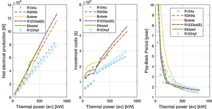
After the analysis presented inTable 6,Fig. 10shows the optimal performance for eachfluid in terms of net electrical production, PBP and Investments costs for a wide range of thermal power input with a PBP optimization. The PBP optimization is selected in this example because of its lower investment costs (seeTable 7) which makes it more interesting for investors. The thermal power input is varied by using the heat sourcefluid mass flow rate according toTable 3. The Pentane is
not shown in the graphs since no feasible solutions were obtained. For a given input thermal power, the best fluid in terms of net electrical production is R1233zd(E) followed by Ethanol, R245fa, Butane, R134a and R1234yf (Fig. 10a). However, the refrigerant R134a presents the lowest investment costs (Fig. 10b), thanks to the lower cost of the screw expander (only allowed with thisfluid) compared with the turbine. The optimal fluid (from a thermo-economic point of view) should present a large net electrical production with low investment costs. The PBP optimization results are shown in Fig. 10c. R134a, R1234yf, R1233zd(E), R245fa and ethanol are the most suitable solu-tions to minimize the PBP depending on the input thermal power.
4.3. Case studies
In s4.1 and 4.2, only the PBP optimization was considered to il-lustrate examples of model application. Both case studies listed in Table 4are optimized in four different ways: to reach the lowest PBP, the highest NPV, the highest IRR and the highest PI (Table 7).
Firstly, it can be noted that the optimal solution is very similar whatever the objective function to optimize among NPV, IRR and PI. The PBP optimization presents different results because of its definition that leads to short term analyses (lower than 3 years in the optimal cases). On the contrary, the NPV, IRR and PI optimizations are based on the typical lifetime of the plant (20 years), which leads to solutions with higher investment costs. The optimal solution for all configurations is with R134a as a working fluid performing a trans-critical cycle and using two screw expanders. This optimum is confirmed byFig. 10c, but it can also be observed that R245fa and Ethanol do lead to close results Fig. 9. Layout of the two case studies. Continuous line arrows correspond to the thermal power available at the component inlet.
Table 5
Results of the optimization for the case study 2 with workingfluid R245fa (PBP opti-mization).
Architecture Subcritical Wet expansion Trans-critical Expander Screw Turbine Screw Screw Turbine Net electrical power [W] 9193 35,022 345 22,809 54,354 Exergy efficiency [–] 0.12 0.26 0.09 0.17 0.29 Evaporation pressure [bar] 32 32.8 25 120 62.8 Refrigerantflow [kg/s] 0.93 1.02 0.32 1.17 1.04 VC [m3/MJ] 1.21 – 1.64 0.59 – SP [m] – 0.02 – – 0.02 PBP [years] – 3.36 – 6.2 2.8
Feasibility No Yes No Yes Yes
Table 6
Optimal architecture and expander for each workingfluid (PBP optimization) for input thermal powers ranging from 50 kW to 800 kW.
Fluid R134a R245fa Butane Pentane R1233zd(E) Ethanol R1234yf
Architecture Transcritical Transcritical Transcritical Transcritical Transcritical Subcritical Transcritical Vaporization enthalpy at 60% of critical pressure [kJ/kg] 113.420 103.038 209.008 192.623 103.590 444.025 107.620
Expander(s) 2 Screws Turbine Turbine Turbine Turbine Turbine 2 Screws
even if slightly disadvantageous.
Comparing these results (Table 7) with the results offluid R1233zd (E) (Table 5) it can be noted that: the turbine (resp. the screw expander) is the optimal solution with R1233zd(E) (resp. R134a), the net elec-trical production is higher for R1233zd(E) (54 kW) than for R134a (33 kW), but the lower investment costs required with R134a leads to a lower PBP of 2.25 years against 2.8 years for R1233zd(E). Regarding the PBP optimization, thefirst case study leads to a 15 kW net electrical production while the second one leads to 33 kW. The optimal condi-tions (pressures and pinch-points) are rather close for each case study. This leads to similar PBP, IRR, PI, LCOE and exergy efficiency. The NPV is larger in the second case study due to the larger installed power.
Finally, a cost and exergy decomposition analysis are proposed for thefirst case study. The fraction of cost and exergy destruction for each component is calculated with the results obtained by the PBP optimi-zation (Screw and R134a–Fig. 11). A general observation is the low
exergy destruction and cost fraction of the pump, even if its importance increases with lower power capacities. In the case of the screw ex-pander, the costs are similar between the condenser, the expander and the evaporator (i.e. high temperature heat exchanger) while in the turbine case, the cost of the expander is predominant. The exergy de-struction is mainly located in the condenser and the evaporator.
Table 8shows the comparison of the obtained results with the ones available in the literature. Since WHR-ORC power systems for biogas application have been investigated scarcely in the past, only 4 papers have been considered[13–16]. It is possible to note inTable 8that the obtained ORC thermal efficiencies are in a realistic range with the va-lues in the literature. The slightly lower vava-lues observed can be ex-plained by the lower thermal input (it depends on the application) and the additional realistic constraints considered in this work.
Regarding the economic analysis, since no studies have been carried out on AD-ORC in the Northern Ireland market, any comparison would be inappropriate. As just a reference,Table 8reports the NPV values calculated by Sung et al.[15]for a biogas micro-turbine system coupled with a subcritical ORC cycle for the South Korean market.
Fig. 10. (a) Net electrical production, (b) investment costs and (c) pay-back period for each workingfluid. Table 7
Results a of the optimization for the two case-studies.
Optimization criteria PBP NPV/IRR/PI
Case study 1 2 1 2
Evaporator secondaryfluid mass flow rate [kg/ s]
0.183 0.3799 0.184 0.362
Architecture Trans-critical
Fluid R134a
Expander(s) 2 Screws
Gas heater pressure [bar] 86.4 85.5 105 112 Condensation pressure [bar] 11.1 11 9 9
Approach [K] 65 18 16 20
Evaporator pinch point [K] 9.8 9.7 16 5 Net electrical power [kW] 15 33 18 38 Exergy efficiency [–] 0.23 0.23 0.26 0.26 Energy efficiency [–] 0.101 0.107 0.121 0.124 Investments costs [k€] 71.4 140.4 96.6 200.6 PBP [years] 2.74 2.25 3.00 2.72 NPV (20 years) [M€] 0.367 0.773 0.399 0.846 Profitability Index [–] 6.1 6.4 5 5 Interest Return Rate [–] 0.44 0.46 0.36 0.37 LCOE [€/kWh] 0.045 0.041 0.052 0.051 Primary energy savings [MWh] 253.8 529.2 287.2 606.7
4.4. Generalization
The optimization procedure was performed for a wide range of heat source fluid flows at the gas heater leading to input thermal powers ranging from 50 kW to 800 kW (seeTable 3).Fig. 12a compares the optimization in terms of PBP and in terms of NPV (Fig. 12). The opti-mization process always leads to the use of R134a as working fluid, except for the circled point where R1233zd(E) showed to be the best choice. The NPV (IRR, NPV or PI) optimization (long term analysis) promotes higher investments with higher PBP and Net Present Value. Investors should therefore choose between high profits on the long terms (IRR/PI/NPV optimization) or lower profits with less risk asso-ciated (PBP optimization). Discontinuities in the plots correspond to different optimal working fluids.
5. Conclusion
This paper presents an investigation on the technical and economic suitability of ORC systems for biogas power plant application (AD-CHP). The investigation was carried out considering different ORC ar-chitectures (i.e. trans-critical, wet expansion and subcritical archi-tecture) and different potential AD-ORC configurations. A thermo-economic tool with an optimization methodology was developed.
The main results obtained are:
– The integration of expander constraints in such thermo-economic optimization has been demonstrated to be mandatory since it limits
the possible solutions severely.
– Neither the wet expansion cycle nor the Pentane are feasible in this case study due to the expander constraints. The integration of other expanders (radial inflow turbine or radial outflow turbine) may enlarge the panel of solutions.
– Some fluids require higher investments (R1233zd(E), R245fa, Ethanol) than R134a and R1234yf but they can achieve higher net electrical production.
– Investors should choose between high profits on the long terms (IRR/PI/NPV optimization) or lower profits with less risk (PBP op-timization). This choice is strictly related to the investors’ invest-ment policy and it can change thefinal design considerably. All these observations are only valid with the assumption and in the range of the parameters considered.
Considering the specific AD-CHP application, for a PBP minimiza-tion two choices are feasible for investors:
– A low investment (€71.4 k) trans-critical ORC power system using R134a as working fluid and two screw expanders. This solution gives an output of 15 kWe with a PBP lower than 2.75 years, a PI of 6.1, a NPV of€366.5 k and an IRR of 44%.
– A higher investment (€139.9 k) with the same fluid and expander. This option leads to a 33 kWe production, a PBP lower than 2.8 years, a PI of 6.4, a NPV of€772.6 k and IRR of 46%.
Form a NPV optimization, two choices are feasible for investors: Table 8
Comparison of the optimization results with literature.
Ref. ORC Architecture Input thermal power [kW]
Exhaust gas temperature [°C]
Workingfluid ORC efficiency [%] NPV [M€]
Mudasar et al.[16] Sub-critical 1000 450 Toluene 12 –
Yangli et al.[14] Sub-critical & trans-critical 510 450 R245fa 15.5/15.9 – Sung et al.[15] Sub-critical 513:1200 250:300 Nepentane 10.2:15.9 1.69–3.378
Di Maria et al.[13] Sub-critical 521 475 Toluene 21.3 –
This paper Sub-critical, wet expansion & trans-critical
148:306 470 Optimization with 7fluids 10.7:12.4 0.43:1.0
– A low investment (€96.6 k) trans-critical ORC power system using R134a as working fluid and two screw expanders. This solution gives an output of 18 kWe with a PBP lower than 3 years, a PI of 5, a NPV of€398.9 k and an IRR of 36%.
– A higher investment (€200.6 k) with the same fluid and expander. This option leads to a 38 kWe production, a PBP lower than 2.8 years, a PI of 5, a NPV of€846.2 k and IRR of 37%.
Acknowledgments
Authors would like to thank the ASME KCORC foundation which promoted the collaboration between the University of Liege and the Queen’s University Belfast.
References
[1] European Union. Energy efficiency directive 2012/27/EU. Off J Eur Union; 2012. [2] De Rosa M, Douglas R, Glover S. Numerical analysis on a dual-loop waste heat
recovery system coupled with an ORC for vehicle applications. SAE Technical Paper. 2016-01-0205; 2016.
[3] Campana F, Bianchi M, Brachini L, De Pascale A, Peretto A. ORC waste heat re-covery in European energy intensive industries: energy and GHG savings. Energy Convers Manage 2013;76:244–52.
[4] Lecompte S, Lemmens S, Huisseune H, Van den Broek M, De Paepe M. Multi-ob-jective thermo-economic optimization strategy for ORCs applied to subcritical and transcritical cycles for waste heat recovery. Energies 2015;8:2714–41.http://dx. doi.org/10.3390/en8042714.
[5] Hærvig J, Sørensen K, Condra T. Guidelines for optimal selection of workingfluid for an organic Rankine cycle in relation to waste heat recovery. Energy 2016;96:592–602.
[6] Yu H, Eason J, Bielger LT, Feng X. Simultaneous heat integration and techno-eco-nomic optimization of Organic Rankine Cycle (ORC) for multiple waste heat stream recovery. Energy 2017:322–33.
[7] Maraver D, Royo J, Lemort V, Quoilin S. Systematic optimization of subcritical and transcritical organic Rankine cycles (ORCs) constrained by technical parameters in multiple applications. Appl Energy 2014;11:11–29.
[8] Glover S, Douglas R, De Rosa M, Zhang X, Glover L. Simulation of a multiple heat source supercritical ORC (Organic Rankine Cycle) for vehicle waste heat recovery. Energy 2016;93:1568–80.
[9] Lemmens S. A perspective on costs and cost estimation techniques for Organic Rankine Cycle systems. In: 3rd International seminar on ORC power systems. Brussels, Belgium; 2015.
[10] Quoilin S, Declaye S, Legros A, Guillaume L, Lemort V. Workingfluid selection and operating maps for Organic Rankine Cycle expansion machines. In: Proceedings of the 21st International Compressor Conference at Purdue; 2012.
[11] Bianco V, De Rosa M, Scarpa F, Tagliafico L. Implementation of a cogeneration plant for a food processing facility. A case of study. Appl Therm Eng 2016;S1359–4311.http://dx.doi.org/10.1016/j.applthermaleng.2016.04.023. 30509-9.
[12] Schuster A, Karellas S, Karakas E, Spliethoff H. Energetic and economic investiga-tion of Organic Rankine Cycle applicainvestiga-tions. Appl Therm Eng 2009;29:1809–17. [13] Di Maria F, Micale C, Sordi A. Electrical energy production from the integrated
aerobic-anaerobic treatment of organic waste by ORC. Renew Energy 2014;66(461):467.
[14] Yangli H, Koç K, Koç A, Georgülü Adnan, Tandiroglu Ahmet. Parametric optimi-zation and exergetic analysis comparison of subcritical and supercritical organic Rankine cycle (ORC) for biogas fueled combined heat and power (CHP) engine exhaust gas waste heat. Energy 2016;111(923):932.
[15] Sung T, Kim S, Kim K. Thermoeconomic analysis of a biogas-fueled micro-gas tur-bine with a bottoming organic Rankine cycle for a sewage sludge and food waste treatment plant in the Republic of Korea. Appl Therm Eng 2017;127:963–74. [16] Mudasar R, Aziz F, Kim M. Thermodynamic analysis of organic Rankine cycle used
forflue gases from biogas combustion. Energy Convers Manage 2017;153:627–40. [17] Santosh Y, Sreekrishnan TR, Kohli S, Rana V. Enhancement of biogas production
from solid substrates using different techniques––a review. Bioresour Technol 2004;95:1–10.
[18] Holm-Nielsen JB, Al Seadi T, Oleskowicz-Popiel P. The future of anaerobic digestion and biogas utilization. Bioresour Technol 2009;100:5478–84.
[19] European Biogas Association, 2015. Biomethane and Biogas Report, Accessible at
www.european-biogas.eu/2015/12/16/biogasreport2015/. [last accessed 15/6/ 2017].
[20] Pöschl M, Ward S, Owende P. Evaluation of energy efficiency of various biogas production and utilization pathways. Appl Energy 2010;87:3305–21. [21] Fischer J. Comparison of trilateral cycles and organic Rankine cycles. Energy
2011;36:6208–19.
[22] Schuster A, Karellas S, Aumann R. Efficiency optimization potential in supercritical Organic Rankine Cycles. Energy 2010;35:1033–9.
[23] Bronicki L. Organic Rankine cycle (ORC) power systems technologies and appli-cations In: History of Organic Rankine Cycle systems; 2016.
[24] Smith IK. Development of the trilateralflash cycle system Part1: fundamental considerations. Proc. Inst. Mech Eng Part A J Power Energy 1993;207:179–94.
[25] Lai NA, Fischer J. Efficiencies of power flash cycles. Energy 2012;44:1017–27. [26] Lecompte S, Huisseune H, Van der Broek M, Vanslambrouck B, De Paepe M. Review
of organic Rankine cycle (ORC) architectures for waste heat recovery. Renew Sustain Energy Rev 2015;47:448–61.
[27] Zhang S, Wang H, Guo T. Performance comparison and parametric optimization of subcritical Organic Rankine Cycle (ORC) and transcritical power cycle system for low-temperature geothermal power generation. Appl Energy 2011;88:2740–54. [28] Astolfi M. Techno-economic optimization of low temperature CSP systems based on
ORC with screw expanders. International Conference on Concentrating Solar Power and Chemical Energy Systems, SolarPACES, Energy Procedia 2014;69:1100–1112. [29] Lecompte S, Lemmens S, Verbruggenb A, Van den Broek M, De Paepe M.
Thermo-economic comparison of advanced organic rankine cycles. Energy Procedia 2014;61:71–4.
[30] Blades L, Morgan K, Douglas R, Glover S, De Rosa M, Cromie T, et al. Circular biogas-based economy in a rural agricultural setting. Energy Procedia 2017;123:89–96.
[31] Questor Centre. Queen’s University Belfast. Northern Ireland Biogas Research Action Plan 2020; , 2014. Report available online at:www.questor.qub.ac.uk[last accessed 10/03/2017].
[32] Guercio A, Bini R. Biomass-fired Organic Rankine Cycle combined heat and power systems, Organic Rankine cycle (ORC) power systems technologies and applica-tions; 2016.
[33] Anaerobic Digestion Bio-resources Association (ADBA); 2017.www.adbiosources. org[last accessed, 21/02/2017].
[34] Northern Ireland Renewable Obligation; 2017. Website:www.economy-ni.gov.uk
[last accessed 10/03/2017].
[35] DECC. UK Department of Energy and Climate Changes; 2017.
[36] Bell I, CoolProp version 5.0; 2016.http://www.coolprop.org/consulted on the 18/ 05/2017.
[37] Öhman H, Lundqvist P. Comparison and analysis of performance using low tem-perature power cycles. Appl Therm Eng 2013;52:160–9.
[38] Quoilin S, van den Broek M, Declaye S, Dewallef P, Lemort V. Techno-economic survey of Organic Rankine Cycle (ORC) systems. Renew Sustain Energy Rev 2012;22:168–86.
[39] Astolfi M, Romano MC, Bombarda P, Macchi E. Binary ORC (Organic Rankine Cycles) power plants for the exploitation of medium–low temperature geothermal sources–Part B: techno-economic optimization. Energy 2014;66:435–46. [40] Dai Y, Wang J, Gao L. Parametric optimization and comparative study of organic
Rankine cycle (ORC) for low grade waste heat recovery. Energy Convers Manage 2009;50:576–82.
[41] Branchini L, De Pascale A, Peretto A. Systematic comparison of ORC configurations by means of comprehensive performance indexes. Appl Therm Eng
2013;61:129–40.
[42] Macchi E. The choice of workingfluid: The most important step for a successful organic Rankine cycle (and an efficient turbine), Keynote lecture. In: Proceedings of the ASME ORC2013, Rotterdam, The Netherlands, 7–8 October 2013; 2013. [43] Lemort V, Legros A. Organic Rankine cycle (ORC) power systems technologies and
applications, Positive displacement expanders for Organic Rankine Cycle systems; 2016.
[44] Quoilin S, Declaye S, Tchanche BF, Lemort V. Thermo-economic optimization of waste heat recovery organic Rankine cycles. Appl Therm Eng 2011;31:2885–93. [45] Gnielinsky V. New equations for heat and mass transfer in turbulent pipe and
channelflow. Int J Chem Eng 1976;16:359–68.
[46] Petukhov BS. Heat transfer and friction in turbulent pipeflow with variable phy-sical properties. Irvine TF, Hartnett JP, editors. Adv Heat Transfer, vol. 6. New York: Academic Press; 1970.
[47] Han D-H, Lee K-J, Kim Y-H. Experiments on the characteristics of evaporation of R410A in brazed plate heat exchangers with different geometric configurations. Appl Therm Eng 2003;23:1209–25.
[48] Han D, Lee K, Kim Y. The characteristics of condensation in brazed plate heat and exchangers with different chevron angles. J Korean Phys Soc 2003;43:66–73. [49] Pioro IL, Duffey RB. Heat transfer & hydraulic resistance at supercritical pressures
in power engineering applications. ASME publication; 2007. ISBN: 0-7918-0252-3. [50] Petukhov BS, Krasnoschekov EA, Protopopov VS. An investigation of heat transfer
tofluid flowing in pipes under supercritical conditions. In: Proceedings of the International Developments in Heat Transfer, University of Colorado, Boulder, CO, USA, 8–12 January, vol. 67; 1961. p. 569–578.
[51] Mokry S, Pioro I, Farah A, King K, Gupta S, Peiman W, et al. Development of su-percritical water heat-transfer correlation for vertical bare tubes. Nucl Eng Des 2011;241:1126–36.
[52] Pucciarelli A, Ambrosini W. Improvements in the prediction of heat transfer to supercritical pressurefluids by the use of algebraic heat flux models. Ann Nucl Energy 2017;99:58–67.
[53] Cavalini A. Heat transfer and heat exchangers, Organic Rankine Cycle (ORC) power systems, Technologies and applications; 2016.
[54] Shah RK, Sekulic DP. Chapter 17-heat exchangers. In: Hartnett JP, Cho YI, Rohsenow WM, editors. Handbook of heat transfer. New York: McGraw-Hill; 1998. [55] Esser A, Sensfuss F. Review of the default primary energy factor (PEF) reflecting the estimated average EU generation efficiency referred to in Annex IV of Directive 2012/27/EU and possible extension of the approach to other energy carriers, consulted the 01/06/2017 onhttps://ec.europa.eu/energy/sites/ener/files/ documents/final_report_pef_eed.pdf; 2012.
[56] Turton R, Bailie RC, Whiting WB, Shaeiwitz J, Bhattacharyya D. Analysis, synthesis and design of chemical processes. 4th ed. Ann Arbor, MI, USA: Pearson Education; 2013.