A two-level emergency control scheme against power system voltage instability
Bogdan Otomegaa, Mevludin Glavicb, Thierry Van Cutsemc
aPower System Department, Politehnica University of Bucharest, 313 Spl. Independentei, 060042, Bucharest, Romania. bDept. of Electrical Engineering and Computer Science, University of Li`ege, Sart Tilman B37, B-4000 Li`ege, Belgium. cFund for Scientific Research& Dept. of Elec. Eng. and Comp. Sc., University of Li`ege, Sart Tilman B37, B-4000 Li`ege, Belgium
(e-mail: t.vancutsem@ulg.ac.be; fax:+ 32 4 366 45 82).
Abstract
A two-level adaptive control scheme against power system voltage instability is proposed, to deal with emergency conditions by acting on distribution transformers and/or by curtailing some loads. The lower level includes distributed controllers, each acting once the voltage at a monitored transmission bus settles below a threshold value. The upper level benefits from wide-area monitoring and adjusts in real-time the voltage thresholds of the local controllers. Emergency detection is based on the sign of sensitivities. The proposed scheme is robust with respect to communication failures. Its performance is illustrated through detailed simulations of a small but realistic 74-bus test system.
Keywords: Power systems, voltage instability, emergency control, distributed control, wide-area monitoring, adaptive systems,
load shedding, load tap changer.
1. Introduction
Voltage instability of power systems is linked to the inabil-ity of the combined generation-transmission system to provide the power requested by loads [1]. In a typical voltage insta-bility scenario, the maximum power deliverable to loads drops under the effects of a large disturbance and the limitations on reactive power generation; concurrently, the loads connected to the transmission system tend to restore their powers near the value before the disturbance. Those antagonistic effects pre-vent the system from regaining a state of operating equilibrium with network voltages in acceptable ranges of values [2]. De-pending on the involved component dynamics and the severity of the disturbance, voltage instability can evolve in time frames of several seconds (short-term instability) or tens of seconds up to several minutes (long-term instability). In this paper, the emphasis is on long-term voltage instability, in which network voltages undergo a generally monotonic decrease after the ini-tiating disturbance.
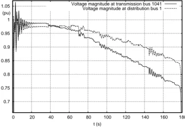
A typical example from simulation is shown in Fig. 1 (ob-tained with the system considered in the results section). The power system is subject to a short-circuit which is cleared by opening a transmission line. The plot shows the evolution of the voltage magnitudes at a transmission and the closest dis-tribution bus1. After the fault is cleared, the system is subject to electromechanical oscillations (of the rotors of synchronous generators) before approaching a short-term equilibrium. Next, the system evolves in the long term under the above mentioned effect of generator reactive power limitation and load power restoration.
1all voltages are shown in per unit (pu), i.e. divided by the nominal voltage of the corresponding bus
0.7 0.75 0.8 0.85 0.9 0.95 1 1.05 0 20 40 60 80 100 120 140 160 180 t (s) (pu)
Voltage magnitude at transmission bus 1041 Voltage magnitude at distribution bus 1
Figure 1: Example of long-term voltage instability
When pronounced, and if not controlled, voltage instability may result in voltage collapse. In the case of Fig. 1 this takes on the form of a loss of synchronism of a nearby generator, leading to the sharp final voltage drop. In practice, this will trigger a sequence of events leading most likely to a blackout. The heavy consequences of power system blackouts in terms of economical and societal costs [3, 4] motivate the improvement of control schemes to deal with voltage instability problems.
Remedies against voltage instability can be categorized into preventive actions and corrective controls.
Preventive actions consists of adjusting the operating point in order the system to be able to face each credible incident (referred to as contingency) of a predefined list. Those ac-tions are taken in normal operating state, i.e. before the
oc-currence of any disturbance, and involve costs to protect the system against hypothetical events. However, many voltage incidents resulted from a severe low-probability disturbance, against which it would be too expensive if at all feasible -to take preventive actions.
Corrective controls aim at acting after the actual occurrence of a disturbance. They can be broadly classified into open-loop and closed-loop. Open-loop control resorts to actions deter-mined off-line from exhaustive simulations of postulated sce-narios while closed-loop control assesses the disturbance sever-ity through measurements, adjusts its actions correspondingly, tracks the system evolution and repeats some actions if the pre-vious ones are not sufficient.
The dominant trend is to integrate emergency controls in Sys-tem Integrity Protection Schemes (SIPS) [5] while exploiting new technological solutions such as synchronized phasor mea-surements [6] and fast communications as the main enablers of power system Wide Area Monitoring System (WAMS) [7]. New algorithms are needed to process the data collected in WAMS and effectively control unstable system evolutions.
This paper deals with such an algorithm. It proposes an adap-tive two-level emergency control scheme aimed at driving the voltage unstable system towards a new, acceptable equilibrium [1]. The lower level consists of distributed controllers acting in closed-loop on loads once the voltages at monitored transmis-sion buses fall (and stay for some time) below threshold values. The upper level takes advantage of a WAMS to detect instabil-ity, and assign their voltage thresholds to the lower-level con-trollers, in the spirit of an adaptive system. The control scheme is robust with respect to controller or telecommunication fail-ures.
The paper is organized as follows. To make the paper self-supporting, some fundamentals of voltage instability and its countermeasures are recalled in Section 2. The lower and upper levels of the proposed scheme are detailed in Section 3 and 4, respectively. Section 5 is devoted to simulation results, while conclusions are provided in Section 6.
2. Voltage instability mechanism and corrective controls This section reviews the basic voltage instability mechanism of a power system subject to a large disturbance [1]. It uses a two-bus system example made as simple as possible while still capturing the main features of instability. Next, the two correc-tive controls considered in this work are briefly described.
2.1. Voltage instability mechanism
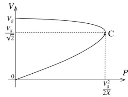
Consider the system in Fig. 2.a in which a generator feeds a load through a transmission line. It is assumed that the gen-erator keeps its terminal voltage Vgconstant and provides any
active power requested by the load. The line is simply repre-sented by its series reactance X. Finally, the load is assumed to have unity power factor, i.e. it does not consume reactive power. The power flow equations of this system are:
P= −VgV X sinθ 0= − V2 X + VgV X cosθ (1) r 1 V2∠θ V∠θ −+ X Vg∠0 V∠θ P X + − Vg∠0 G a. c. b.
Figure 2: Two-bus system and corresponding circuits
V P C V2 g 2X Vg √ 2 Vg 0 x
Figure 3: Network PV curve (load with unity power factor)
where all symbols are defined in Fig. 2.b. Combining these two equations, the voltage V at the load bus is easily obtained as:
V= v u t V2 g 2 ± √ V4 g 4 − X 2P2 (2)
The variation of V with P is shown in Fig. 3 where the up-per (resp. lower) part of the curve corresponds to the solution with the+ (resp. the −) sign in (2). Such a plot is referred to as “PV curve” by power system engineers. The load power is maximum at point C, also called “critical” point. The maximum deliverable power is PC= V2 g 2X under voltage VC = Vg √ 2. Load dynamics play an important role in voltage instability. In the long-term time frame, loads are controlled by Load Tap Changers (LTCs). These devices adjust the turn ratios of the transformers feeding distribution systems in order to keep the voltages at the distribution sides of the transformers close to a set-point. LTCs can act in discrete steps only, corresponding to the available transformer tap positions. They remain the main voltage control means in distribution systems, although this task is expected to be shared by distributed generation units in future smart grid architectures [8, 9].
To illustrate the LTC effect, in Fig. 2.c, the load of our two-bus system has been replaced by a load at distribution level be-hind a step-down transformer. In line with the previous simpli-fications, this transformer is assumed ideal, thus:
V2= V
r (3)
C A O V P disturbance r↓ x Po long-term short-term
Figure 4: Voltage instability explained with (network and load) PV curves
where r is the transformer ratio and V2the distribution voltage. Furthermore, a constant conductance load is considered:
P= GV22= G (V r )2 (4) Let Vo
2 be the voltage set-point of the LTC. Whenever V2falls below Vo
2 − ϵ (resp. raises above V
o
2 + ϵ), the LTC decreases (resp. increases) r in order to bring back V2in the dead-band [Vo
2− ϵ V
o
2 + ϵ]. r is changed step by step with delays between changes. The dead-band is needed for proper operation with a limited number of tap positions.
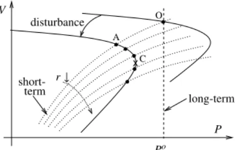
Network and load characteristics are combined in Fig. 4. As-sume that the system operates initially at point O. The dotted line passing through O is the transient load characteristic, cor-responding to (4), while the vertical dashed line is the steady-state load characteristic. In steady steady-state, assuming that the LTC has restored V2= V2o(neglecting the effect of ϵ), the load power is P= Po= G(V2o)2. Thus, by controlling distribution voltages, LTCs make loads appear constant power in steady state.
The remaining of the figure illustrates a typical instability scenario. A severe disturbance, such as the outage of a trans-mission equipment, increases X so much that the new maxi-mum deliverable power (corresponding to point C) falls below
Po, the power initially consumed by the load, that the LTC will try to restore indirectly. Since the long-term load characteristic does no longer intersect the network PV curve, it can be con-cluded that the system has lost its equilibrium. This will result in the following unstable evolution. Right after the disturbance, the new operating point is A, at the intersection of the short-term load and network post-disturbance characteristics. At this point, the load power is smaller than Po, which means that V
2is smaller than Vo
2. Hence, the LTC will decrease r in successive steps. As can be seen from (4), each new value of r yields a new short-term load characteristic. The intersections of those characteristics with the network PV curve give the successive operating points shown with dots in Fig. 4: in its unsuccessful attempt to restore the distribution voltage, the LTC depresses the transmission voltage V. After crossing the maximum power point C, the tap changes are even counterproductive!
A similar behaviour is observed in Fig. 1 where the distribu-tion voltage (dashed line) cannot be restored in the correspond-ing [0.99 1.01] pu dead-band.
Expectedly, some features of voltage instability are not shown in the above simplistic example [1, 10]:
• an excessive decline of voltages is unacceptable since it may cause further equipment (in particular loads) to trip or it may trigger a faster instability such as loss of synchro-nism or motor stalling (see the final evolution in Fig. 1); • generators are not pure voltage sources. In normal
condi-tions, the terminal voltage of a synchronous generator is tightly controlled by its automatic voltage regulator. How-ever, if keeping that voltage constant requires producing too much reactive power, the generator field current may exceed its thermal limit and be reduced after some delay by an Over-Excitation Limiter (OEL) to avoid equipment damages. The resulting loss of voltage control by a gen-erator has a similar effect as the initiating outage: the PV curve further shrinks, and the maximum power deliverable to the load further decreases;
• besides LTCs, there are other load power restoration mech-anisms such as the control of heating loads by thermostats.
2.2. Corrective controls
The above simple example suggests directly two types of cor-rective controls, which are considered in this paper:
1. modified LTC control: to stop the degradation caused by LTCs. Standard emergency actions consist of blocking tap changers on their current positions, moving them to pre-determined positions, or reducing the voltage set-points
Vo
2 [10–12]. In this paper a more advanced control is con-sidered which involves a transmission voltage preserving logic [13];
2. load shedding: moves the long-term load characteristic to the left, in Fig. 4, so that a new intersection with the net-work PV curve is created. Curtailing a proper amount of interruptible load at the proper place and in appropriate time is a very effective countermeasure against voltage in-stability [10, 14–18]. It is needed when system voltages drop too much immediately after the disturbance, the LTCs being to slow to move. At the price of disconnecting some loads, the others quickly regain normal voltage. Shedding is actuated by opening distribution circuit breakers; finer control of individual appliances is envisioned in the con-text of demand response management in smart grids [8, 9]. The above corrective controls affect the quality of power sup-ply, and, hence, are envisaged in severe situations only. Less in-trusive controls, to be actuated in priority, consist of increasing generator voltages (though in a limited interval) or connecting shunt capacitors (if available) to the transmission bus feeding the load. Both actions increase to some extent the maximum power deliverable to the load. A more detailed discussion of emergency voltage stability controls can be found in [19, 20].
3. Lower-level distributed control of load shedding and tap changers
3.1. Distributed control
The design of an emergency control scheme against voltage instability must address a number of issues:
• the magnitude of the corrective action needed to stabilize the system is not known beforehand;
• saving the system from a blackout is the priority. To this end, the corrective action can be slightly in excess, in ex-change for other advantages such as reliability. Never-theless, since corrective control is intrusive from the con-sumer viewpoint, it should be as small as possible; • real-life power systems include a large number of loads
and generators. The regions exposed to voltage instability are known by transmission system operators. However, inside those regions, it is not known beforehand where it is most appropriate to act. This is even more true for well meshed networks;
• loads are the most effective components to act on. How-ever, in practice, there is much uncertainty regarding their behaviour. For instance, when opening a distribution cir-cuit breaker, the controller does not necessarily know how much reactive power is going to be curtailed together with the active power, and how much the power of the remain-ing loads will vary with the voltage increase;
• the scheme must be robust with respect to failures of sen-sors or actuators. This requires some form of redundancy. Most of the above issues are addressed by resorting to a set of controllers distributed over the region of interest, and operating in closed-loop. “Closed-loop operation” refers to the ability for a controller to act in successive steps, each decision relying on the measured result of previous actions. The distributed design allows adjusting corrective control to the disturbance location [21]. It also provides redundancy, since in case of failure of one controller, the others can take over [22].
Two additional features of the distributed controllers con-tribute to making the scheme simple and, hence, more reliable: • the controllers do not exchange information, but are rather informed of their respective actions through the power sys-tem itself. This is made possible by the absence of “iner-tia” in voltage dynamics: in the time frame of concern, it can be considered that the effects of one controller are instantaneously felt by the others;
• the controllers do not need any system model.
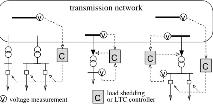
In the sequel a combination of distributed load shedding and LTC controllers is considered, as sketched in Fig. 5. Each load shedding controller monitors the voltage V at a transmission bus and acts on a set of loads at distribution level, located close enough to the monitored bus, so that their curtailment allows in-creasing V. Each LTC controller measures the voltage of both the transmission and the distribution terminal of the transformer it is controlling. In normal operating conditions, it regulates the distribution voltage as usual, while in emergency conditions, it preserves the transmission voltage. The remaining of this sec-tion is devoted to presenting these controllers in greater detail.
load shedding voltage measurement transmission network or LTC controller v v v v C C C C v v C v
Figure 5: Distributed control of load shedding and tap changers
STARTED SHED
IDLE and t− t
0< τ
V< Vth V< Vthand load can be curtailed
[ set t0to current t ]
V≥ Vth V≥ Vth
[ set t0to current t ]
V≥ Vthor no more load can be curtailed
V< Vthand load can be curtailed
and t− t0≥ τ
V< Vth or load can
no longer be curtailed
Figure 6: Logic of individual load shedding controller. Within brackets: action taken when the transition takes place [22]
3.2. Load shedding controller
Each load shedding controller relies on the simple rule:
IF V< Vth during time τ , shed load power ∆P (5) A more precise description is given by Fig. 6 in the form of an automaton. As long as V remains above Vth, the controller is idle, while it is started as soon as a disturbance causes V to drop below Vth. Let to be the time where this change takes place.
The controller remains started until either the voltage recovers, or the timeτ is elapsed since to. In the latter case, the controller
sheds a power∆P and returns to either idle (if V recovers above
Vthor no more load can be shed) or started state (if V remains
below Vth and there remains load to shed). In the second case,
the current time is taken as the new value of toand the controller
is ready to act again.
The choice of Vthwill be discussed in detail in Section 4. As regardsτ and ∆P, they can be adjusted to the severity of the situation, assessed through the amplitude of Vth− V [22]. In
fact, our analysis of many cases has shown that smallτ and ∆P values, i.e. shedding with little delay and in small steps, usually lead to shedding less load. It also makes the system recover more smoothly. Thus, constant, pre-defined values ofτ and ∆P are considered in this paper. Note thatτ must be large enough so that the controller does not to react to a short-circuit on the transmission system. Indeed, after the fault has been cleared by protections, the voltage takes one or two seconds to recover a normal value.
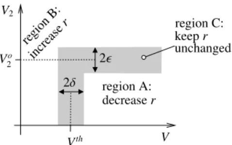
region C: region A: 2ϵ V Vth region B: increase r decrease r V2 Vo 2 2δ unchanged keep r
Figure 7: LTC control combining DVR and TVP logics
DOWN STARTED IDLE DECREASE RATIO r UP STARTED INCREASE RATIO r enters A stays in A and t− to≥ τ stays in A stays in A and t− to< τ leaves A leaves A OR r=rmin leaves B OR r= rmax enters B leaves B stays in B stays in B and t− to≥ τ in C OR stays in B and t− to< τ (in A AND r= rmin) OR (in B AND r= rmax)
*
*
*
*
Figure 8: Combined DVR-TVP logic of individual LTC controller. A, B and C refer to the regions of operation in Fig. 7. A star (*) indicates that tois set to
current time t when the transition takes place. “rmin” (resp. “rmax”) denotes the minimum (resp. maximum) value of the ratio. For clarity, adjustments of τ (different delays before first and between subsequent tap changes) are not shown.
3.3. Load Tap changer controller
With the transformer ratio defined as in Fig. 2.c, a standard LTC controller monitors the distribution voltage V2and modi-fies the ratio r as follows: decrease r if V2 < V2o− ϵ, increase r if V2 > V2o+ ϵ, and leave it unchanged otherwise. A more advanced control logic is considered here, in which the trans-mission voltage V (on the high-voltage side of the transformer) is also monitored with respect to a threshold value Vth. As long
as V remains above Vth+ δ the LTC operates in the above,
stan-dard manner. On the contrary, if V falls below Vth − δ, the
LTC stops regulating the distribution voltage and, instead, pre-serves the transmission voltage by increasing r. If V lies in the [Vth−δ Vth+δ] range, the tap changer does not move; this
dead-band prevents from oscillating between the Distribution Voltage Regulation (DVR) and the Transmission Voltage Preservation (TVP) logics. The above rules are summarized in Fig. 7 while the combined DVR-TVP logic is presented in automaton form in Fig. 8.
The choice of Vth is discussed in detail in Section 4. The
dead-band 2ϵ is unchanged with respect to usual LTCs, with a typical value in the range of 2 %. The dead-band 2δ can be given the same value.
3.4. Automatic shunt compensation switching
As already mentioned, this paper focuses on LTC control and load shedding. However, the switching of shunt compensa-tion (switching on capacitors - switching off reactors) is han-dled similarly, and can be described in similar terms. Usu-ally, several capacitor banks are available in a substation. Once the transmission voltage V falls below Vth, the local controller
switches one bank at a time, after a delay similar toτ in Fig. 6.
4. Upper level: emergency detection and voltage threshold adjustment
4.1. Motivation for an upper level
In spite of their advantages, the distributed controllers still rely on the particular value assigned to Vth. This voltage
thresh-old should not be set too high, to avoid triggering corrective control at normal voltages, or at low but stable voltages. It should not be set too low either, since it will lead to act later and, hence, expose the system to degraded operating conditions for a longer time. Also, when delayed, the corrective actions have to be more pronounced [1], which results in sharper volt-age corrections. Finally, Section 5.5 will give an example where it is impractical to rely on Vthwithout further information.
This leads to complementing the distributed controllers with an upper level in charge of sending Vth values - or equivalent
information - in real-time, when emergency conditions and im-pending instability are detected.
The aim of an upper-level controller in a hierarchical con-trol scheme is typically to coordinate the efforts of lower-level controllers or to adjust their parameters adaptively. The latter option is considered in this work. By adjusting Vthin response
to the particular disturbance faced, the upper level provides the whole scheme with the basic feature of an adaptive system.
To this purpose, the upper level is assumed to embed a WAMS receiving real-time measurements [7]. In the future, WAMS are expected to benefit from the progress made in syn-chronized phasor measurement technology [6].
4.2. Implementation
Following a large disturbance, the role of the upper level is to detect that the system is evolving towards long-term volt-age instability, more precisely to identify that the system has crossed a “critical voltage profile”. The latter defines the low-est acceptable voltage Vthat the various buses monitored by the
lower-level controllers. This way of doing is justified by the ob-servation that a long-term voltage unstable system undergoes a monotonic decrease of voltages, as illustrated by Fig. 1. Then, the role of the distributed controllers will be to restore and maintain their monitored transmission voltages at or slightly above the critical voltage profile.
This can be performed with very little information sent from upper to lower level (virtually a single bit of information!). In-deed, at the time the upper level detects that the system has crossed the critical voltage profile, it sends a signal to the lower-level controllers requesting each of them to take its currently measured voltage V as threshold value Vth. Each controller acts
independently from the others to restore V ≥ Vth.
If, for any reason, the upper level monitoring scheme fails providing the signal to the local controllers, the latter may use their original (preset) thresholds. This redundancy increases the reliability of the whole protection.
4.3. Detecting an impending instability
The simple example in Fig. 4 suggests taking for Vth the
voltage VC at the critical point C. Indeed, at this point, the
load power is restored to the greatest possible extent. Before crossing C, the transmission voltage V is depressed by the tap changes but in exchange for a restoration of the distribution voltage V2, while after crossing C both transmission and dis-tribution voltages are depressed.
The method detailed in [23] can be used to identify the criti-cal point in the general case involving multiple loads and multi-ple generators, some of them getting limited. It is summarized hereafter.
A set of algebraic equations:
ϕ(z, s) = 0 (6)
is fit to the sampled states, where z denotes the state vector and
s the vector of load active and reactive powers. These equations
are obtained under the following assumptions:
• the network is represented by its bus admittance matrix, using real-time breaker status information;
• the short-term dynamics of generators, automatic voltage regulators, speed governors, static var compensators, etc. are replaced by accurate equilibrium equations;
• whether a generator is voltage controlled or limited by its OEL is either known from measurements or detected from computation of the field current.
Sensitivities identify when a combination of load active and reactive powers passes through a maximum. This requires knowing the consumed powers only: no model of load be-haviour with voltage is needed. Sensitivities of the total reactive power generation Qgto the load reactive powers are considered.
They are obtained by differentiation of (6) as [20]: ∂Qg ∂q = − ( ∂ϕ ∂q )T (∂ϕ ∂z )T −1 ∂Qg ∂z (7)
where q is the vector of load reactive powers, which is a sub-vector of s.
At the maximum load power point, one real eigenvalue of ∂ϕ
∂z changes sign. Hence, in theory, the sensitivities change sign
passing through infinity. In practice, the critical point crossing is identified at a discrete time k such that, for at least bus j:
∂Qg
∂qj
(k− 1) > d and ∂Qg ∂qj
(k)< −d (8)
where d> 0 is a properly chosen threshold.
It is essential to reflect any change of generator voltage con-trol in the equations (6). An estimate of Eq, the e.m.f.
propor-tional to field current, is used to identify whether a synchronous generator operates under control of its Automatic Voltage Reg-ulator (AVR) or has been already limited by its OEL. Under AVR control, an equation such as:
kEsq− G(Vo− V) = 0 (9)
is used, while under OEL control, it is replaced by an equation of the type:
Eq− Elimq = kEqs− Elimq = 0 (10)
where G is the open-loop static gain of the AVR, Eqsis the e.m.f. behind saturated synchronous reactances, k is the saturation fac-tor, V is the terminal voltage, Vois the AVR voltage set-point, and Elimq corresponds to the field current forced by the OEL. Eq
and k are components of z together with bus voltages and other variables.
The most important feature of the sensitivities is their ability to anticipate the effect of an approaching OEL activation. To this purpose, when Eq exceeds Eqlim, the OEL equation (10) is
anticipatively substituted to the AVR equation (9) before eval-uating ∂ϕ
∂z. More details can be found in [23]. The anticipation capability is illustrated in the next section.
4.4. Real-time measurement requirements
The above sensitivities are intended to be computed on suc-cessive “snapshots” of the evolving system state. For each snap-shot, the complex voltages at the various buses should be esti-mated (at least in the region of interest). This is typically the role of a state estimator running in the control center. In the authors’ simulations, the rate at which measurement samples are processed is high compared to the capability of present day static state estimators. Therefore, extensions towards tracking state estimation have to be considered. In this respect, the emer-gence of the time synchronized phasor measurement technol-ogy opens new perspectives, as detailed in [24], for instance.
Further discussion of this important issue is beyond the scope of this paper. Note, however, that sensitivity computation and monitoring can be replaced by a simpler (more conservative) detection of emergency voltage conditions. In the two-level scheme proposed in this paper, what is eventually sought is an emergency signal sent to the lower-level controllers.
5. Simulation results
5.1. Test system
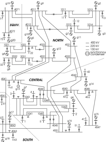
The performance of the proposed controller is illustrated on the 74-bus, 20-generator, 22-load Nordic32 system. Its one-line 6
g15 g11 g20 g19 g16 g17 g18 g2 g6 g7 g14 g13 g8 g12 g4 g5 g10 g1 g3 g9 4011 4012 1011 1012 1014 1013 1022 1021 2031 cs 4046 4043 4044 4032 4031 4022 4021 4071 4072 4041 1042 1045 1041 4063 4061 1043 1044 4047 4051 4045 4062 400 kV 220 kV 130 kV synchronous condenser CS NORTH CENTRAL EQUIV. SOUTH 4042 2032 41 1 5 3 2 51 47 42 61 62 63 4 43 46 31 32 22 11 13 12 72 71
Figure 9: One-line diagram of the Nordic32 test system
diagram is shown in Fig. 9. This small but realistic test system has been used in several references, for instance [22, 23].
The results were obtained from time simulations of the sys-tem model under the phasor approximation, typical of power system stability studies [25]. This model involves close to 700 differential and algebraic states (including the 148 real and imaginary components of the 74 complex bus voltages) Each generator is equipped with an OEL in charge of limiting its field current after a delay that may depend on the thermal overload. Each of the 22 loads is fed through a distribution transformer equipped with LTC. The LTCs have various delays: on the av-erage, 30 s on the first tap change, and 10 s between subse-quent changes. There are around 250 discrete states in limiters, switches, LTC discrete-time controllers, etc.
5.2. Disturbance
The disturbance of concern is a short-circuit at t= 1 s on line 4032-4044. This fault is cleared after 0.1 s (5 cycles at 50 Hz) by opening the faulted line, which remains opened. As the ini-tial operating state is insecure, the outage of that line makes the system long-term voltage unstable.
5.3. Lower-level distributed controllers
To counteract voltage instability, the system has been pro-vided with five load shedding controllers, distributed over the
130-kV network of the Central area, where the most pro-nounced voltage drops are experienced. These controllers mon-itor voltages at buses 1041, 1042, 1043, 1044, and 1045, respec-tively, and shed load at the corresponding distribution buses 1, 2, 3, 4 and 5 (see Fig. 9). Each controller sheds load in steps ∆P of 10 MW (with a corresponding decrease of the reactive power) and with a delayτ of 3 seconds.
In replacement of, or in complement to load shedding, the combined DVR-TVP logic detailed in Fig. 8 has been consid-ered for the LTCs controlling the same five buses. δ has been set to 0.01 pu, which is also the value ofϵ (see Fig. 7).
5.4. Results with exponential load models
The results of this subsection have been obtained assuming that all loads follow the so-called exponential model [25]:
P= Po (V Vo )α Q= Qo (V Vo )β (11) where V is the corresponding distribution bus voltage, Vo the
initial value of V, Po (resp. Qo) the initial load active (resp. reactive) power.α = 1, β = 2 was chosen for all loads.
Uncontrolled system response
The long-term unstable evolution of the uncontrolled system has been shown in Fig. 1. It is driven by the LTCs and by a cascade of OEL activations taking place between t = 55 and
t= 147 s, on g12, g14, g7, g11, g6, g15 and g16, successively.
Instability detection at upper level
At the upper level, the sensitivities (7) are used as explained in Section 4. The z vectors have been obtained from snapshots of the bus voltage phasors provided by time simulation.
The evolution of the sensitivity ∂Qg ∂qj
relative to bus 1041 is shown in Fig. 10. A single bus is considered for clarity, but it is proved in [23] that the sensitivities change sign altogether (at least at buses most impacted by instability).
The solid line correspond to the sensitivity evaluated “with-out OEL anticipation”, i.e. accounting for the field current lim-itation of a generator after its OEL has acted. The change in sign takes place at t= 87 s. Assuming a one-second delay to as-certain that the sensitivities settle to negative values, the emer-gency signal is sent by the upper level at t= 88 s. The dashed line shows the sensitivity computed “with OEL anticipation”, i.e. accounting for the near-future limitation of a generator as soon as the field current exceeds its limit. The change in sign occurs at t= 72 s, i.e. 15 s earlier.
When receiving the emergency signal, each lower-level con-troller takes the transmission voltage it currently measures as threshold value Vth. Since the sensitivities give an early
warn-ing, some of these voltages can still be high. Considering that emergency control is intrusive for customers, Vthhas been
Figure 12: Evolution of load powers (shedding actions are identified with∗)
Table 3: Power curtailments (in MW) with inter-level communication failures
No failure Case A Case B
bus Vth power Vth power Vth power
(pu) shed (pu) shed (pu) shed
1041 0.93 20 0.93 40 0.93 80 1042 0.95 0 0.95 0 0.95 0 1043 0.95 50 0.95 50 0.95 130 1044 0.92 30 0.92 100 0.90 0 1045 0.94 100 0.90 0 0.90 0 Total 200 190 210
The LTC operation is illustrated in Fig. 14, relative to trans-former 1041-1. The figure shows the trajectory of the system superimposed to the diagram of Fig. 7. The large transients due to the initial short-circuit have been removed for clarity. The pre-disturbance operating point is O, with the voltage at the distribution bus 1 in its dead-band. At t ≃ 30 s, when the sys-tem has almost settled to a short-term equilibrium (see Fig. 1), but before the LTC starts acting, the operating point is A. The unsuccessful operation of the LTC leads to point B. Then, the situation is aggravated by the field current limitation of genera-tors g14 and g7, leading to point C. This makes the LTC enter the TVP region of operation. The reverse tap changes preserve transmission to the detriment of distribution voltage, until the LTC eventually settles at point D in the dead-band.
Comparison
When resorting to load shedding, some loads are discon-nected while the others regain a normal voltage value. With LTC control, the effort is shared by all loads, whose powers decrease under the effect of depressed voltages. These two ac-tions on loads can be compared considering, for load shedding, the total curtailed power and, for LTC control, the non-restored load power [13]: ∆Pnr = ∑ i∈I ( Poi − Pif inal) (12)
Figure 13: Evolution of voltage at bus 1041 with DVR-TVP control of LTCs (two variants) 0.88 0.9 0.92 0.94 0.96 0.98 1 1.02 1.04 0.88 0.9 0.92 0.94 0.96 0.98 1 1.02 1.04 1.06
Voltage at bus 1 (pu)
Voltage at bus 1041 (pu) O A B C D decrease r increase r keep r unchanged
Figure 14: System trajectory in the (V1041, V1) space (voltages at the transmis-sion and distribution ends of transformer 1041-1)
where Po
i is the pre-disturbance active power of the load at the
i-th bus, Pif inal is the corresponding value in the final steady state, and I is the set of distribution buses whose voltage is outside the LTC dead-band.
The values of∆Pnrand the contribution of each bus are given
in Table 4 for the two stabilized evolutions shown in Fig. 13. The values of∆Pnrare comparable to the total curtailed powers
detailed in Table 2.
5.5. Results in the presence of induction motor loads
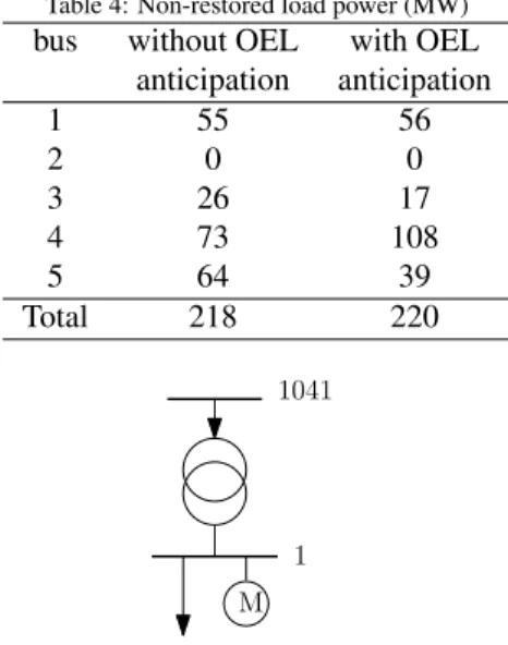
The performance of the proposed scheme has been tested in more stringent conditions, assuming that the loads at buses 1, 2, 3, 4, 5, 43, 46, and 47 include 40 % of induction motors. To this purpose each of these eight loads has been split into a part represented with the previous exponential model, taking 60 % of the initial active power, in parallel with an equivalent (single cage) induction motor, as shown in Fig. 15, relative to bus 1. Each equivalent motor accounts for many motors connected to the distribution system. It is represented by a set of three dif-ferential and two algebraic equations, with parameters typical of large industrial motors [10]. Shedding is applied to the non-motor part of the loads.
Table 4: Non-restored load power (MW)
bus without OEL with OEL
anticipation anticipation 1 55 56 2 0 0 3 26 17 4 73 108 5 64 39 Total 218 220 M 1041 1
Figure 15: Composite load model including an equivalent motor
Uncontrolled system response
The evolution of the voltage at bus 1041, under the effect of the same disturbance, is shown with solid line in Fig. 16. For comparison purposes, the figure shows with dotted line the response which was obtained with fully exponential load model, see Fig. 1. In the presence of motors, the voltage drop is sharper. It takes place earlier, when the voltage support of key generators is lost due to OEL action, which causes the mo-tors to stall [1, 10]. The task of designing emergency control is more delicate because: (i) a few seconds before collapsing, voltages still have normal values, and (ii) the decrease is so fast that prompt corrective actions are needed.
Instability detection at upper level
The evolution of the component of SQgqrelative to bus 1041
is shown in Fig. 17. Without (resp. with) OEL anticipation, the change in sign takes place at t= 68 s (resp. t = 53s).
The values of Vth taken by the controllers when receiving
the upper-level emergency signal are given in Table 5. With OEL anticipation, the emergency was detected so early that all voltages were still above the upper bound of 0.95 pu.
Stabilization by DVR-TVP control of LTCs
The effect of LTCs operating according to the combined DVR-TVP logic is shown in Fig. 18. Even though the signal is received very early, the LTCs control actions are too slow to prevent the sharp voltage decay. They only succeed postponing voltage collapse a little, at the cost of pronounced oscillations.
Stabilization by load shedding
Failure to stabilize the system also takes place when resorting to distributed load shedding controllers with Vth = 0.90 pu, as
previously considered (see Table 2). Indeed, withτ set to three seconds, the controllers react too late to stabilize the system. Reducingτ is not an option due to the risk of unduly shedding load after a short-circuit normally cleared by protections [26].
0.65 0.7 0.75 0.8 0.85 0.9 0.95 1 1.05 0 20 40 60 80 100 120 140 160 180 t (s) (pu)
loads with induction motor representation loads represented with exponential model
Figure 16: Unstable evolution of voltage at bus 1041 in the presence of induc-tion motor loads and with exponential load models
-60 -40 -20 0 20 40 60 80 100 120 0 10 20 30 40 50 60 70 t (s)
sensitivity computed without anticipation sensitivity computed with anticipation
Figure 17: Evolution of the sensitivity∂Qg ∂qj
relative to bus 1041
Successful stabilization is obtained by combining load shed-ding with the upper-level early detection of emergency. The stabilized voltage evolution is shown in Fig. 19, for both sets of
Vth values given in Table 5. The smoother evolution obtained
with the higher Vthsettings is noteworthy.
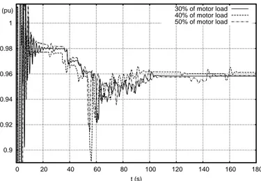
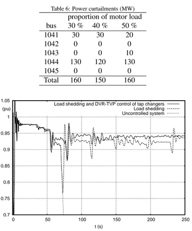
Figure 20 shows the performance of the same load shedding scheme for 30, 40 and 50 % of motor load, respectively. Table 6 shows the corresponding power curtailments. The protection scheme performs very similarly in all three cases, which reveals some robustness with respect to load behaviour uncertainty.
Stabilization by both LTC control and load shedding
To deal with such severe situations, it is reasonable to com-bine both types of corrective control. This is illustrated in Fig. 21. The curve with solid line shows the voltage evolu-tion that result from DVR-TVP control of LTCs, based on the
Vth values in the third column of Table 5, together with load
shedding, based on the Vthvalues in the second column of the
same table. Thus, LTC control is activated first, followed by 10
Table 5: Voltage thresholds Vth(in pu)
bus without OEL with OEL
anticipation anticipation 1041 0.91 0.95 1042 0.95 0.95 1043 0.93 0.95 1044 0.91 0.95 1045 0.93 0.95 0.65 0.7 0.75 0.8 0.85 0.9 0.95 1 1.05 0 20 40 60 80 100 120 t (s) (pu)
DVR-TVP control of LTCs - Vth determined without OEL anticipation DVR-TVP control of LTCs - Vth determined with OEL anticipation Uncontrolled system
Figure 18: Unsuccessful system stabilization by DVR-TVP control of LTCs
load shedding. The dashed curve, reproduced from Fig. 19, corresponds to load shedding only. The reduction of distribu-tion voltages by LTCs leads to shedding only 60 MW, instead of 220 MW when LTCs are not used for emergency control. In this combined scheme, two signals would be sent by the upper level, intended to LTCs and load shedding, respectively.
6. Conclusion
A two-level adaptive control scheme against power system voltage instability has been proposed.
At the lower level, it relies on a set of distributed controllers, acting when (and as long as) monitored transmission voltages are below threshold values. Upon detection of an emergency situation, the upper level sends a signal to the distributed con-trollers, for the latter to set their threshold values at the currently measured voltages. The objective is to keep system voltages above the critical profile corresponding to the emergency de-tection. The distributed controllers adjust their actions to the severity and location of the disturbance.
The emergency signal is obtained from wide-area monitoring by the upper level. To this purpose, an advanced sensitivity-based analysis has been considered.
The results obtained with the small but realistic Nordic32 test system have confirmed the following expectations:
• proper adaptation of the voltage thresholds in real time yields a more dependable protection;
0.7 0.75 0.8 0.85 0.9 0.95 1 1.05 0 50 100 150 200 250 t (s) (pu)
Load shedding - Vth determined without OEL anticipation Load shedding - Vth determined with OEL anticipation Uncontrolled system
Figure 19: Evolution of voltage at bus 1041 with load shedding (two variants)
0.9 0.92 0.94 0.96 0.98 1 0 20 40 60 80 100 120 140 160 180 t (s)
(pu) 30% of motor load
40% of motor load 50% of motor load
Figure 20: Evolution of voltage at bus 1041 with load shedding, for three pro-portions of motor load
• the proposed scheme is fault-tolerant since it accommo-dates failures to receive the emergency signal;
• the early emergency signal sent by the upper level allows acting fast enough in case of sharp voltage drops caused by motor loads, a situation where relying on local voltages is not sufficient.
Two types of emergency controls were considered. While modified control of load tap changers can help in slowly de-creasing voltage situations, it has to be replaced or, even better, complemented by load shedding to counteract the faster insta-bility caused by induction motor loads.
Automatic shunt compensation switching can be also in-cluded, and should be given priority as it is less intrusive for the consumers.
Acknowledgment
B. Otomega has been financially supported by the Sectoral Operational Programme Human Resources Development
2007-Table 6: Power curtailments (MW) proportion of motor load
bus 30 % 40 % 50 % 1041 30 30 20 1042 0 0 0 1043 0 0 10 1044 130 120 130 1045 0 0 0 Total 160 150 160 0.7 0.75 0.8 0.85 0.9 0.95 1 1.05 0 50 100 150 200 250 t (s)
(pu) Load shedding and DVR-TVP control of tap changersLoad shedding Uncontrolled system
Figure 21: Evolution of voltage at bus 1041 with DVR-TVP control of LTCs and load shedding
2013 of Romanian Ministry of Labor, Family and Social Pro-tection through Agreement POSDRU/89/1.5/S/62557.
References
[1] T. Van Cutsem, C. Vournas, Voltage Stability of Electric Power Systems, Springer (previously Kluwer Academic Publishers), Boston, 1998. [2] P. Kundur, J. Paserba, V. Ajjarapu, G. Andersson, A. Bose, C. Ca˜nizares,
N. Hatzyargyriou, D. Hill, A. Stankovic, C. Taylor, T. Van Cutsem, V. Vit-tal, Definition and classification of power system stability, IEEE Trans. Power Syst. 19 (2004) 1387–1401.
[3] US-Canada Power System Outage Task Force, Final report on the August 14, 2003 blackout in the United States and Canada: Causes and recom-mendations, [Online]. Available: reports.energy.gov.
[4] Union for the Co-ordination of Transmission of Electricity, Final re-port: System disturbance on 4 November 2006, [Online]. Available: www.entsoe.eu.
[5] V. Madani, D. Novosel, S. Horowitz, M. Adamiak, J. Amantegui, D. Karlsson, S. Imai, A. Apostolov, IEEE PSRC report on global industry experiences with system integrity protection schemes (sips), IEEE Trans. Power Del. 25 (2010) 2143–2155.
[6] A. G. Phadke, J. S. Thorp, Synchronized Phasor Measurements and their Applications, Springer, New York NY, 2008.
[7] A. Phadke, R. M. de Moraes, The wide world of wide-area measurement, IEEE Power and Energy Mag. 6 (2010) 52–65.
[8] J. Momoh, Smart Grid: Fundamentals of design and analysis, Wiley-IEEE Press, Hoboken NJ, 2012.
[9] A. P. S. Meliopoulos, G. Cokkinides, R. Huang, E. Farantatos, S. Choi, Y. Lee, X. Yu, Smart grid technologies for autonomous operation and control, IEEE Trans. Smart Grid 2 (2011) 1–10.
[10] C. W. Taylor, Power System Voltage Stability, EPRI Power System Engi-neering Series, McGraw Hill, New York, 1994.
[11] C. Vournas, G. Manos, Emergency tap-blocking to prevent voltage col-lapse, Proc. 2001 IEEE PES PowerTech Conference, Porto, Portugal. [12] C. Vournas, M. Karystianos, Load tap changers in emergency and
pre-ventive voltage stability control, IEEE Trans. on Power Systems 19 (Feb. 2004) 492–498.
[13] B. Otomega, V. Sermanson, T. Van Cutsem, Reverse-logic control of load tap changers in emergency voltage conditions, Proc. 2003 IEEE PES PowerTech Conference, Bologna, Italy.
[14] C. W. Taylor, Concepts of undervoltage load shedding for voltage stabil-ity, IEEE Trans. Power Del. 7 (1992) 480–487.
[15] B. Ingelsson, P. Lindstrom, D. Karlsson, G. Ruvnik, J. Sjodin, Spe-cial protection scheme against voltage collapse in the South part of the Swedish grid, Proc. CIGRE Conf.
[16] Z. Feng, V. Ajjarapu, D. J. Maratukulam, A practical minimum load shed-ding strategy to mitigate voltage collapse, IEEE Trans. Power Syst. 13 (1998) 1285–1291.
[17] C. Moors, D. Lefebvre, T. Van Cutsem, Load shedding controllers against voltage instability: a comparison of designs, Proc. 2001 IEEE PES Pow-erTech Conference, Porto, Portugal.
[18] V. C. Nikolaidis, C. D. Vournas, Design strategies for load shedding schemes against voltage collapse in the hellenic system, IEEE Trans. Power Syst. 23 (2008) 582–591.
[19] C. Vournas, A. Metsiou, M. Kotlida, V. Nikolaidis, M. Karystianos, Com-parison and combination of emergency control methods for voltage sta-bility, Proc. IEEE PES 2004 General Meeting, Denver, USA.
[20] T. Van Cutsem, C. D. Vournas, Emergency voltage stability controls: An overview, Proc. IEEE PES 2007 General Meeting, Tampa, USA. [21] F. Capitanescu, B. Otomega, H. Lefebvre, V. Sermanson, T. Van Cutsem,
Decentralized tap changer blocking and load shedding against voltage in-stability: Prospective tests on the rte system, Int. Journal Elec. Power and Energy Syst. 31 (2009) 570–576.
[22] B. Otomega, T. Van Cutsem, Undervoltage load shedding using dis-tributed controllers, IEEE Trans. Power Syst. 22 (2007) 1898–1907. [23] M. Glavic, T. Van Cutsem, Wide-area detection of voltage instability from
synchronized phasor measurements. Part I: Principle. Part II: Simulation results, IEEE Trans. Power Syst. 24 (2009) 1408–1425.
[24] M. Glavic, T. Van Cutsem, Reconstructing and tracking network state from a limited number of synchrophasor measurements, IEEE Trans. Power Syst. 28 (2013) 1921–1929.
[25] P. Kundur, Power System Stability and Control, The EPRI power system engineering series, McGraw-Hill, 1994.
[26] B. Otomega, T. Van Cutsem, A load shedding scheme against both short-and long-term voltage instabilities in the presence of induction motors, Proc. 2011 IEEE PES PowerTech Conference, Trondheim, Norway.