Anisotropic elasto-plastic finite element analysis using a stress-strain
interpolation method based on a polycrystalline model
Anne Marie Habraken, Laurent Duchêne
University of Liège, Department of Mechanics of Materials and Structures, Chemin des Chevreuils, 1, Bât B52I3, 4000 Liège, Belgium
Abstract
This paper describes a stress-strain interpolation method to model the macroscopic anisotropic elasto-plastic behavior of polycrystalline materials. Accurate analytical descriptions of yield loci derived from crystallographic texture [Int. J. Plasticity 19 (2003) 647; J. Phys. IV France 105 (2003) 39] are an interesting alternative to finite element models, where the macroscopic stress is provided by an averaging of microscopic stresses computed on a set of representative crystallites [Acta Metal 22 (1985) 923; Int. J. Plasticity 5 (1989) 67]. The parameters of the analytical functions modeling the yield locus are identified by comparison with a high number of stress tensors computed, for instance, by the well-known Taylor model [J. Inst. Metal 62 (1938) 307]. This identification method depends on the crystallographic texture and should be applied each time that the plastic strain has induced a significant texture evolution. The stress-strain interpolation method accurately describes the anisotropic material behavior in a narrow stress direction defined by only five stress points. The cost of texture updating is then greatly reduced compared to a full analytical function of the yield locus. After the mathematical description of the stress-strain interpolation method, its validity is demonstrated on two non-radial strain paths. The simulations of a deep drawing experiment allow comparing model predictions and
measurements. Accuracy and CPU time of the interpolation stress-strain method are judged against two other models, respectively based on a complete analytical yield locus and on the averaging of crystallite stresses. Keywords : B. anisotropic material ; B. constitutive behavior ; B. polycrystalline material ; C. cinite elements ; C. crystallographic texture
1. Introduction
Plastic anisotropy is considered as an essential feature to provide accurate finite element (FE) predictions of metal forming processes. As macroscopic behavior results from microscopic events, a logical scientific approach was to develop crystalline-plasticity-based FE simulations. A lot of averaging methods are possible to extract the macroscopic behavior from microscopic analyses applied to a representative set of crystallites (Aasro and Needleman, 1985; Mathur and Dawson, 1989; Neale, 1993; Lebensohn and Tome, 1993; Beaudoin et al., 1995; Anand et al., 1997; Molinari, 1997; Nakamachi et al., 2000, 2002; Li et al., 2003; Van Bael and Van Houtte, 2003). Section 2 provides a description of the typical features of micro-macro models in order to define the background of the developed innovative method. The present paper describes an efficient way to integrate into a macroscopic anisotropic elasto-plastic FE code the effect of polycrystalline texture evolution with a limited number of computations at the microscopic level. At each FE integration point, a set of representative crystallites characterized by their updated orientations defines the anisotropy of the material. Micro-macro transition is assumed by the simplest and most widely used approach to obtain the response of a polycrystal from the response of individual grains: iso-deformation gradient in all the crystallites representing the polycrystals (Full Constraints Taylor model; Taylor, 1938). The single crystal behavior is computed according to the Taylor-Bischop-Hill crystal model (TBH). The Taylor assumptions and simplifying hypotheses of the TBH theory are recalled in Sections 3.1 and 3.2. They have been implemented in the FE code LAGAMINE developed by the M&S department. The micro-macro transition provides macroscopic stress tensors (stress nodes) defining the yield locus in the interesting zone of the yield locus. As long as the stress direction is not modified, the current stress tensor is computed by the stress-strain interpolation method based on these stress nodes. These nodes are updated from time to time according to the texture evolution. New stress nodes are required when stress direction changes. This method is described in Sections 3.3-3.7. Compared to other micro-macro methods, it significantly reduces the CPU requirements, while preserving the full accuracy of texture updating. Close to local descriptions of the yield locus [multi-dimensional piece-wise linear representation of the yield surface proposed by Maudlin et al. (1996) or Hill-ellipsoids used to locally approximate the polycrystal stress potentials by Tóth et al. (1996)], this method is however different. As discussed in Section 3.5, this interpolation approach only approximately follows classical yield locus description and normality rule. In Section 4, academic
validations on two non-radial strain paths are presented. Predictions around bi-axial state are analyzed by comparison with the response directly computed by Full Constraints Taylor method. Section 5 consists in the comparisons of FE results and measurements of a deep drawing experiment. Accuracy and CPU time are
compared to models based on complete analytical yield locus or averaging of crystallite stresses. Finally, Section 6 concludes and offers perspectives for the continuation of this research.
2. General micro-macro framework
The goal of this section is far from giving a complete state-of-the-art of micro-macro models. However the stress-strain interpolation method is situated between two types of models, one that relies on analytical yield locus functions and the other that averages crystallite stresses. The features of these two types of models are recalled hereafter. More details are given on the Taylor model and the sixth order series yield locus as these methods are compared to the stress-strain interpolation method. Only micro-macro models applied in FE simulations of forming processes are presented. This section does not introduce the refined micro-macro models focused on material behavior. For instance, how to recover the Hall Patch effect (Evers et al., 2002), or
precipitation hardening (Garmestani et al., 2002) or how to accurately take into account grain interactions (Crumbach et al., 2001a,b; Delannay et al., 2002).
2.1. Micro-macro models without analytical macroscopic yield locus
In the case of these micro-macro models, the response of each integration point of the FE mesh depends on the response of a multitude of single crystallites representative of this material point. Such an approach can be applied only with the help of massive parallel computations, when actual deep-drawing simulations of macroscopic pieces are performed. Different models have been developed depending on the chosen crystal plasticity constitutive law and the micro-macro link used. The three most popular micro-macro assumptions are the Taylor hypothesis, the self-consistent model and the FE2 method, where two scales of FE simulations appear. The main features of these model families are recalled hereafter.
In the Full Constraints Taylor assumption (Taylor, 1938), the micro-macro link is such that the local velocity gradient in each crystallite is homogeneous and identical to the macroscopic velocity gradient. This approach respects geometric compatibility between crystallites, but leads to equilibrium violation at crystallite boundaries. Different versions of the Taylor model appear if all the components of the crystal velocity gradient are not constrained to be equal to the macroscopic ones (see Van Houtte et al., 2002, for the analysis of some different solutions). Macroscopic FE simulations have often been coupled with the Full Constraints Taylor version. Such polycrystalline models are described for instance by Asaro and Needleman (1985), Neale (1993), Beaudoin et al. (1994), Kalidindi and Anand (1994), Anand et al. (1997). The differences between all these papers consist in their crystal model and their representative set of crystals. A crystal model is characterized by its choices: to neglect (Mathur and Dawson, 1989) or not elastic behavior (Anand et al., 1997), to use a strain rate dependent crystal plasticity model (Beaudoin et al., 1994) or an elasto-plastic constitutive model (Anand and Kothari, 1996), to assume (Mathur and Dawson, 1989) or not (Anand et al., 1997), an identical Critical Resolved Shear Stress (CRSS) for all slip systems, to apply or not an accurate hardening model for the CRSS as defined by Asaro and Needleman (1985). The choice of a representative set of crystals is also not straightforward and can provide discrepancies between the model results, as underlined by Kallend et al. (1991) or Toth and Van Houtte (1992). The FE simulation results compared with experiments have validated this type of model for b.c.c. and f.c.c. metals (Neale, 1993; Kalidindi and Anand, 1994; Beaudoin et al., 1994). It generally provides accurate predictions of geometry, stress and strain histories during any forming processes. The texture predictions generally show a qualitative agreement, although intensity values are seldom reached.
Texture evolution is directly implemented in this approach where the orientations of the representative crystals are updated according to plastic deformation. Texture evolution is responsible for the "geometrical hardening" also called "textural hardening" (Miller and Mc Dowell, 1996). It modifies the anisotropic shape of the yield locus during deep-drawing processes. On the other hand, the increase of dislocation density constitutes an obstacle to the production and motion of further dislocations. This phenomenon is perceived as the "material hardening" of the crystals. The evolution function of the Critical Resolved Shear Stress of each slip system implemented in the microscopic model can provide an accurate "material hardening" description. It mainly affects the size of the yield locus. With a Taylor type model, Kalidindi (2001) demonstrates that to quantitatively capture the behavior of low stacking fault energy f.c.c metals, "textural" and "material" hardening are not sufficient. It is necessary to incorporate micro-scale shear banding in the crystal plasticity modeling framework. The second possibility of micro-macro link in models without analytical macroscopic yield locus is the self-consistent approach (Berveiller and Zaoui, 1978; Molinari et al., 1987; Molinari, 1997). It considers each crystal as a solid inhomogeneity embedded in a homogeneous infinite matrix subjected to macroscopic loading. Each crystal, one by one, is treated that way and the matrix behavior has to be the average of the contribution of all crystals. At the microscopic level, this method fulfills neither compatibility nor equilibrium between grains, but it takes into account the interactions of grains with the general homogenized medium from a statistical point of view.
Applying Eshelby's (1957) formula, Kröner (1961) studies elastic cases. The extension to nonlinear behavior is still a source of scientific controversy and intensive developments as summarized by Molinari et al. (1987, 1997), Toth and Molinari (1994), Molinari (1997), Masson and Zaoui (1999), Gilormini et al. (2002), Sabar et al. (2002). In metallic polycrystals, a self-consistent method is often applied to hexagonal materials. Their low number of deformation modes bring them far from a homogeneous strain distribution inside and between the crystallites like in the Taylor assumption. Some specific developments of the Taylor model have been proposed for such materials, as in Parks and Ahzi (1990) or Prantil et al. (1995). However, scientists often prefer to use self-consistent approaches in these cases. For instance, Chastel et al. (1998) presents an application of the viscoplastic self-consistent polycrystalline model from Lebensohn and Tomé (1993) coupled to a 3D eulerian FE code applied to the hot extrusion of zircalloy.
Like the Taylor model, the self-consistent approach directly considers both "textural" and "material" hardening in FE simulations. Its advantages are that heterogeneity of strain distribution between crystallites, grain shape and grain interaction can be taken into account at the microscopic level.
The third type of micro-macro models without analytical macroscopic yield locus is the FE2 method based on a homogenization technique where two levels of FE models are coupled (Smit et al., 1998; Miehe et al., 1999; Geers et al., 2000; Elbououni et al., 2003). At each integration point of the macroscopic FE mesh, the
macroscopic constitutive law is computed by another microscopic FE model discretizing a set of representative crystals [Representative Volume Element (RVE)]. With this approach, both equilibrium and compatibility between crystallites are reached in the RVE.
The homogenization theory provides the mathematical background to pass from the microscopic level to the macroscopic level. The advantages of this approach are that texture evolution, grain shape or size effects, grain interaction, heterogeneous stress and strain distributions are directly taken into consideration.
Now that the advantages of each of the three methods have been defined above, their cost should be investigated. For one integration point of the mascroscopic FE mesh and one macroscopic strain rate, the CPU time of the Taylor approach is directly proportional to the number of representative crystals associated with each integration point. The two other methods perform identical microscopic computation as the Taylor model, but a higher number of times as the self-consistent method requires an iterative procedure to define the strain distribution between crystals and the FE2 method solves a nonlinear FE problem to find it.
2.2. Micro-macro models with analytical macroscopic yield locus
In order to reduce computation time, micro-macro FE models with analytical macroscopic yield locus have been investigated. A first option is to develop new macroscopic elasto-plastic or elasto-visco-plastic models with general features imbued from plasticity models in single crystals (Aifantis, 1987; Ning and Aifantis, 1996; Khan and Cheng, 1996, 1998). In this case, no microscopic model is coupled with the macroscopic FE model.
Another possibility is to identify an accurate analytical expression of the yield locus outside the FE code by numerous calls of the Taylor or the self-consistent micro-macro models. Then this accurate yield locus function is used during macroscopic FE computations without any crystal computation.
The size evolution and the position of this yield locus are defined by macroscopic isotropic and kinematic hardening rules. Such hardening models are macroscopic ones but can present strong links to microscopic phenomena (Teodosiu and Hu, 1995, 1998; Miller and Mc Dowell, 1996). However they cannot provide a description as accurate as the one proposed at the crystal level. So these analytical yield loci approximate "material" hardening and neglect "textural hardening" as the link between texture and yield locus shape is performed only once, with the initial texture.
Different ways to derive an analytical yield function from crystal plasticity and texture knowledge have been proposed. The approach of Lequeu et al. (1987) fits an analytical function on the TBH single crystal locus associated with one texture component. When the material has more than one texture component, this model assumes identical microscopic and macroscopic stresses. Darrieulat and Piot (1996) apply the same type of approach; however they consider a more accurate representation of the microscopic behavior and take into account the Orientation Distribution Function (ODF) to represent the texture effect. Arminjon et al. (1994) present a method to identify their analytical plastic power dissipation function from the ODF and the crystal plasticity model. Then, they derive a yield locus applied to polycrystalline metals. When a quadratic form is assumed, the macroscopic anisotropic parameters become explicit functions of the ODF coefficients. Recently, Darrieulat and Montheillet (2003) have also proposed a quadratic yield surface with parameters analytically derived from the orientations and volume fractions of the texture components. As this method is computationally efficient, it can be repeated at various stages of the process to take into account texture evolution.
Imbault and Arminjon (1993) propose a semi-analytical method to handle the texture evolution effect in their analytical expression of the yield locus. The principle is simple: they assume that a linear operator identified by a polycrystalline model can express the evolution of the ODF coefficients with strain.
Van Houtte (1994a) uses the dual plastic potentials to derive convenient formulas of yield loci of rate insensitive anisotropic materials. Van Bael et al. (1996) and Munhoven et al. (1997) have checked that 6th order polynomial series yield locus are required to reproduce the accuracy of polycrystalline approaches. They propose to define this sixth order series yield locus by a least square fit on a large number of points (typically 70 300) in the deviatoric stress space. These points are calculated by the Taylor model based on an assumed constant texture (Van Bael, 1994; Munhoven et al., 1996). This identification is performed once, outside the FE code (Winters, 1996). It provides 210 coefficients to describe the whole yield locus. This model called 'Ani3vh' is compared to the stress-strain interpolation model in Section 5. Unfortunately, taking into account the texture evolution effect with this yield locus means the computation of the 210 coefficients of the sixth order series for each integration point, each time a texture updating is necessary. Recently, Hoferlin et al. (1999) have extended this approach in the strain rate space and coupled it with the microstructural hardening model from Teodosiu and Hu (1995). Li et al. (2003) apply this constitutive model to investigate the effects of texture and strain-path changes on the plastic anisotropy in sheet metal forming.
3. Stress-strain interpolation in a local zone of the yield locus 3.1. Taylor type microscopic plasticity model
As the focused applications are forming processes of steel or aluminium sheets at room temperature, dislocation glides are the main plastic deformation mechanism.
For f.c.c cases, the Miller indices allow defining the 12 slip systems {111} 110 potentially activated and for b.c.c. cases, 24 slip systems are taken into account: {110} 111 and {112} 111 . A classical Taylor microscopic model has been implemented, and its main characteristics are recalled hereafter.
At the crystal level, the components of Ls, the plastic microscopic velocity gradient generated by a particular slip system s, are given by:
where is the slip rate acting on this slip system s and the Schmid tensor Ks is defined by its component Ksij.
with ns unit vector normal to the slip plane and bs unit vector in the slip direction. In practice, multiple slips occur together. Hence Lmicro, the microscopic plastic velocity gradient applied on a crystal, is given by:
where ΩL is the rate of crystal lattice rotation. It can be split into a microscopic plastic deviatoric strain rate
micro and a microscopic spin Ωmicro:
where As and Zs are respectively the symmetric and skew-symmetric parts of the Schmid tensor Ks. The first term of right Eq. (5), is called plastic spin Ωp. Several different combinations of slip rates may achieve the prescribed strain rate. According to Taylor (1938), the one which minimizes power dissipation is chosen:
Taylor roughly assumes that all slip systems have a common value τc of their Critical Resolved Shear Stress τcs,
A weaker hypothesis proposed by Van Bael (1994) is applied, which consists in using proportional CRSS τcs
For instance, for b.c.c crystals the following values are used (Van Bael, 1994):
The prescribed strain rate can be split into a scalar magnitude and a strain rate mode: . Introducing also the slip rate per unit equivalent strain rate:
advantage can be taken of the assumed strain-rate insensitivity to simplify the formulation. Indeed, dividing Eq. (6) by the strain rate magnitude and the reference CRSS τc leads to the Taylor factor M:
with according to Eq. (4), the minimization constraint:
These two equations are called the Taylor equations and may be solved efficiently by means of linear
programming (Simplex Method), as explained by Van Houtte (1988). This approach has been implemented in the LAGAMINE code by Munhoven et al. (1997). The solution depends only on the prescribed strain mode
and not on the magnitude nor on the value of the reference CRSS τc. The Simplex Method produces both
slip rates and microscopic stresses at the crystallite level. In practice, using nearly identical CRSS for all slip systems leads to multiple solutions (set of activated slip systems). Each set achieves the prescribed strain rate Eq. (4) with the same minimum power dissipation Eq. (6). Van Houtte (1988) proposes different methods to choose one particular solution. The approach implemented by Munhoven et al. (1997) just stops at the first computed solution. From an energy point of view, all the solutions are equivalent. However, they produce different slip rates and hence different crystallite lattice rotations. Once the set of active slip systems and the corresponding slip rates are known by the resolution of Eqs. (10) and (11), the crystal rotation ΩL produced by one imposed microscopic velocity gradient can be reached using Eq. (5).
The effect of work hardening is assumed identical for all the slip systems and the reference CRSS evolution is directly linked by a Swift law to Γ, the total slip happening in the crystallite:
where Kτ, Γ0, n are material parameters. The rate of the total crystal slip is computed from the equivalent strain rate and M the Taylor factor, characteristic of the applied strain mode and the crystallite orientation:
3.2. Taylor type micro-macro model
Knowing the initial texture by its Orientation Distribution Function, the selection of a set of 2000 representative crystallites is performed by ODFLAM software (Van Houtte, 2002). At each interpolation point of the FE mesh, the material is characterized by the orientations of these 2000 crystallites. Macroscopic stress and strain
computations are performed in local axes following the material axes. Real material axes attached to a deforming body are subjected to distortion, while local axes remain Cartesian. So, there is no unique definition of a local frame. However the various possible choices differ only through a spurious rigid body rotation. In LAGAMINE code, the method implemented to follow material axes is due to Munhoven et al. (1996). Working in hypo-elastic formulation, constitutive equations are not required for a plastic spin. This choice of hypo-elastic formulation has different advantages and remains physically sound as long as the elastic strains are small. A discussion on this choice can be found in Hoferlin (2001). Hoferlin et al. (1999) links the method proposed by Munhoven to the one presented by Ponthot (1995 or 2002). For each FE integration point, the local axes are computed to provide a macroscopic constant symmetric velocity gradient at each FE time step. The elastic deformation is taken into account on a macroscopic level by the Hooke law. Precisions are given in Section 3.6 describing the stress integration scheme. The macroscopic stress nodes used in the stress-strain interpolation method are computed by a micro-macro model of Taylor type. The microscopic and macroscopic plastic velocity gradients, expressed this time in each crystallite axes, are assumed identical:
So, the plastic deformation and global rotation respectively used in Eqs. (4) and (5) are known. The macroscopic isotropic hardening behavior is taken into account at the crystallographic level through an identical CRSS for all the grains and all the slip systems, the average polycrystal slip rate is directly reached if crystal Taylor factor is replaced by its average value and Eq. (12) can be easily extended:
The macroscopic hardening stress-strain curve (σ-εplastic) identified by a tensile test:
can be converted into a microscopic CRSS-induced slip curve (τc - ).
The microscopic Taylor model described in Section 3.1 is applied for each crystallite and provides the
microscopic stress and the rotation of each representative crystallite. The macroscopic stress is computed by the average of the 2000 microscopic stresses and the updated texture is directly known by the updated angles of the 2000 crystallites.
3.3. Definition of a local zone of the scaled yield locus
Shape and size of the yield locus are separated; only shape is focused on here, as the simple isotropic hardening relation Eq. (16) defines the yield locus size. The yield locus is described in a five-dimensional space because for metals, the plastic strain rate is classically assumed to be deviatoric and only the deviatoric stress tensor matters with regard to plastic deformation (Van Bael et al., 1996). As the deviatoric stress tensor and the plastic strain rate tensor have only five independent components, they are replaced by five-dimensional vectors. Hereafter, the choice of notation is adapted to the stress space, but the whole approach can be transposed into the strain rate space. In all the developments, the subscript * identifies a unit vector. Let s0
*
be one unit deviatoric stress vector, in the central direction of the described local part of the yield locus, si* are five unit deviatoric stress vectors
called the "domain limit vectors", surrounding s0*. They determine the studied local zone of the scaled yield
locus. These six vectors (five si* and one s0*) determine a regular domain, when they have following properties:
These choices induce that the "central" direction s0* can be computed as a scaled average of the five "domain
limit vectors" si*. Both the angle θ and the parameter β are related to the size of the interpolation domain. They
are linked by the relation β2= sin2 θ. As the five si* vectors are linearly independent, they constitute a covariant
vector basis of the five-dimensional space. However, as they are not orthogonal, it is interesting to introduce five new vectors si called "contravariant vectors" with the following orthogonality property:
The five η-coordinates representing any vector v in the si* vector basis are defined by:
and they are easily determined thanks to the five si vectors:
These five independent η-coordinates determine both the length and the direction of the vector v. The "domain limit vectors" represent the domain vertices. The five boundaries (or edges) of the interpolation domain correspond to functions such that:
In fact, the usual properties of intrinsic coordinates associated with isoparametric FEs are retrieved in this approach but extrapolated to five dimensions. The above choices imply that any point belonging to the
interpolation domain is associated with positive η-coordinates.
One convenient way to determine the five "domain limit vectors" si* is to use a two step procedure. First, a
particular "central" direction s'0* is defined and intermediate "domain limit vectors" si* are computed:
where vector ei, is the Cartesian basis, β is the scalar defined by Eq. (17) and α is determined thanks to the
unitary conditions of s'0* and s'i*∙ The second step consists in determining the rotation between the actual
required "central" point s0* and the particular one s'0* and then in applying this rotation to the s'i* vectors to
provide the required domain limit vectors si*.
Such an interpolation domain is called a regular one because the angles between the domain limit vectors are identical [see Eq. (17)] and the domain limit vectors are unit vectors. However, it is possible to define an interpolated domain based on limit vectors that are non-uniformly spaced and non-unit vectors, as long as they are linearly independent. The extension of the above considerations to this case is trivial.
3.4. Stress-strain interpolation method
Now, let us consider the five dimensional stress and strain rate spaces. A regular domain is built in the strain rate space. It is defined by five vertices ui* (unit vectors). Thanks to five calls to the Taylor modules from Sections
3.1 and 3.2 applied on the set of 2000 representative crystallites, the associated stress vectors si can be defined.
At this level, no hardening is assumed; only the shape of a scaled yield locus is described. However as the anisotropy is taken into account, si vectors are of course not unit vectors. These five stress vectors define a
non-regular domain in the stress space. In both spaces, the concept of contravariant vectors of Eq. (19) is applied:
The contravariant vectors si respectively computed by Eqs. (25) and (19) differ because sj is not a unit vector in
Eq. (25) and does not fulfill Eq. (17). Here the length of the stress vectors sj is an important characteristic as it
defines the yield locus anisotropy. The contravariant vectors si and ui give in each space, the η-coordinates associated to any stress s or unit strain rate u*:
Physically, one material state corresponds to one stress point and one strain rate direction. In a stress yield locus formulation, one point on the locus and its normal define a stress and its associated strain rate. Here, we work with two interpolation domains respectively in strain rate space and in stress space. They are physically linked because the Taylor models of Sections 3.1 and 3.2 have computed their domain limit vectors. Due to this close link between the two spaces, it is assumed that the η-coordinates computed by Eqs. (26) and (27) are equal when the stress s and the strain rate direction u* are physically associated. The stress-strain interpolation approach directly derives from this hypothesis of equality. This assumption is exactly fulfilled only for the "domain limit vectors". Here, the stress si corresponds to the strain rate direction ui* and their η-coordinates are ηi = 1 and ηj =
0 (i ≠ j) in both spaces. If any strain rate direction u* is chosen, equality of Eqs. (26) and (27) as well as the η-coordinates definition, Eq. (20) provides the interpolation relation:
For each domain, the C matrix is computed once from the stress domain limit vectors si and the contravariant
vectors ui associated to the five strain rate vertices ui
*
. Inside one domain, Eq. (28) provides the stress state s if the strain rate direction u* is given. The η-coordinates computed by Eq. (26) check the domain validity; their values must belong to the interval [0,1]. Otherwise the interpolation approach defined by Eq. (28) becomes an extrapolation and a new domain is required.
This stress-strain interpolation can be seen as a linear interpolation in "extended" spherical coordinates. For Von Mises yield locus, the domain limit vector lengths are identical and Eq. (28) results in a stress of identical length.
This local approximation of the yield locus is not an hyperplane but a curved surface that exactly fits the stress computed by the Taylor model only at the domain limit vectors.
3.5. Updating of the local scaled yield locus description
When the available local description of the scaled yield locus no longer covers the interested zone, i.e. when the new stress state s falls outside the domain defined by the five si one has to find another local description
enclosing the interesting part of the yield locus. Of course, the procedure to identify the five domain limit vectors described in the previous section [see Eq. (23)] could be repeated using one new central direction. However, this would provide a new local description ignoring previous information and discontinuities would appear.
Looking at the η-coordinate no longer belonging to [0,1], one can identify the crossed boundary by the new explored direction. This boundary is defined by four domain limit vectors. It belongs to two adjacent domains, each defined by five limit vectors, four being common. So, the two neighbor domains defined by their common boundary require only one additional domain limit vector to be completely defined. Only one new vertex must be computed by the Taylor models (Sections 3.1 and 3.2) to identify the neighbor domain probably containing the new explored direction. In the implementation of the stress-strain interpolation method in the LAGAMINE code, the neighbor domain is always checked before the computation of a completely new local domain is considered. The stress continuity between adjacent domains is fulfilled. However this continuity is of the C0
type, so the local yield locus normals are not continuous. Consequently, on the boundary between two domains, two yield locus normals can be computed. The first one comes from the derivatives of the approximate yield locus applied to the first domain; the second one is computed by the same equations but applied to the second domain. If these two normals on the boundary are divergent, the stress will tend to be localized on this boundary because all the plastic strain rate directions included between these two normals will correspond to a stress on this boundary. On the other hand, a locally non-convex yield locus corresponds to the two convergent normals. This case is more inconvenient and leads to numerical instability and convergence problems.
In order to avoid such difficulties, another way for the computation of the normal to the local yield locus is applied. The normal is computed by a weighted average of the plastic strain rate present at the domain limit points. The weight factors are the intrinsic coordinates ξi of the explored stress direction:
The plastic strain rate at each vertex of the domain is already known because it was the input of the Taylor models during the construction of the interpolation domain. This choice avoids the problem of different normals at the boundary between adjacent domains. It is in agreement with the Taylor models at the vertices of the domain but not inside the domain, where the Taylor theory is only approximated. As the normality rule inside the local yield locus description is not fulfilled, this approach could be seen as a local non-associated plasticity model.
3.6. Stress integration scheme
At this level, the real stress and not the scaled one is targeted. So the size and the shape of the yield locus can no longer be dissociated. As Eq. (28) gives the shape and is assumed to model a reference level of hardening, an additional factor τ is introduced to represent the isotropic work hardening:
Here, the CRSS defined by Eq. (15) plays the role of the isotropic hardening parameter.
The deviatoric stress-strain interpolation Eq. (30) does not use the concept of yield locus in a classical way. So, a specific integration scheme different from the classical radial return with elastic predictor has been developed. During an FE simulation, for a plastic loading, Eq. (30) and following classical relation Eq. (31) must be fulfilled:
where t is the time, σ the Cauchy stress, Ce the Hooke elastic matrix. Eq. (31) represents Hooke's law and the objective time derivative of Jaumann is used.
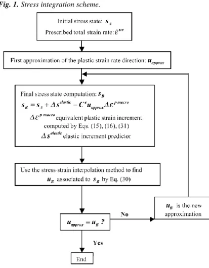
The main ideas of the stress integration scheme are summarized in the flowchart of Fig. 1, where subscripts A and B respectively identify the step beginning and step end, s is the deviatoric stress, ∆ identifies an increment happening during the step.
Δεplastic, equivalent plastic strain increment, is computed by some algebraic developments based on Eqs. (15),
(16) and (31). As it was observed during several FE simulations, this stress integration scheme is well adapted for the chosen local yield locus description and induces a reasonable number of interpolation domain updates.
Fig. 1. Stress integration scheme.
3.7. Implementation of the texture updating
In this model, the texture is used to predict the anisotropic plastic behavior of the material and the strain history of each integration point is taken into account in order to update the texture. The main ideas of the
implementation are summarized in Fig. 2. The crystallographic orientations are represented with the help of the Euler angles ranging from 0° to 360° for φ1 and from 0° to 90° for and φ2 in order to take crystal cubic
symmetry into account but not the sample symmetry. As shown in Fig. 2, the texture updating can independently be activated for each integration point.
During a complete FE simulation, it is not reasonable to perform a texture updating for each integration point at the end of each time step. That is the reason why an updating criterion must be used to reduce computation time. This point is still under investigation. At this stage, an updating simply occurs after a predefined number of time steps. A criterion based on a maximum accumulated plastic strain will be examined.
When texture updating occurs, for each integration point, the lattice rotation of each crystallite belonging to the representative crystallite orientations set is computed by the Taylor models described in Sections 3.1 and 3.2.
Fig. 2. Coupling scheme for texture updating.
4. Academic validations
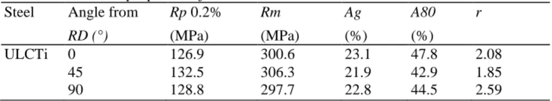
The sheet used in the academic validations is a 0.8 mm thick, Ultra Low Carbon Titanium steel sheet. Table 1 provides its mechanical properties. RD means Rolling Direction, Rp is the elastic limit, Rm the maximum plastic stress, Ag the strain associated to Rm, A80 the strain corresponding to failure, r the Lankford coefficient. K=559.58 MPa, n=0.3054, ε0=0.004594 are the material parameters defining the hardening behavior [Eq. (16)].
The Young modulus and the Poisson ratio are respectively 157 242 Mpa and 0.36. The measured texture exhibits a γ fiber, typical for rolled steels. The maximum value of the ODF is 10.91.
Table 1 Mechanical properties of ULC Ti steel sheet
Steel Angle from Rp 0.2% Rm Ag A80 r
RD (°) (MPa) (MPa) (%) (%)
ULCTi 0 126.9 300.6 23.1 47.8 2.08
45 132.5 306.3 21.9 42.9 1.85
90 128.8 297.7 22.8 44.5 2.59
4.1. Biaxial stress state
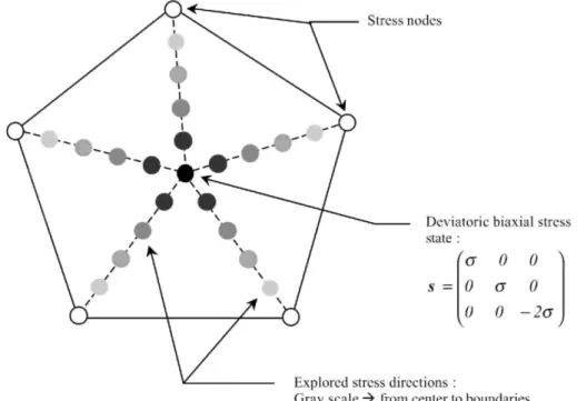
For one particular domain, the computed yield stresses from the stress-strain interpolation method and from an improved hyperplane method are compared to the yield stresses directly computed by the Taylor models from Sections 3.1 and 3.2. The improved hyperplane method simply consists in approximating the yield locus by five hyperplanes, each defined on the central direction s0 and four of the five domain limit vectors si. The particular
chosen domain is centered on the deviatoric biaxial stress state, where generally a strong curvature appears in the yield locus. Fig. 3 presents a schematic representation of the local domain and explains the method used to perform this accuracy test. The relative error on the yield stresses between the results of the local approaches and the Taylor models is computed for 21 points: in addition to the central point of the domain (the biaxial state), 20
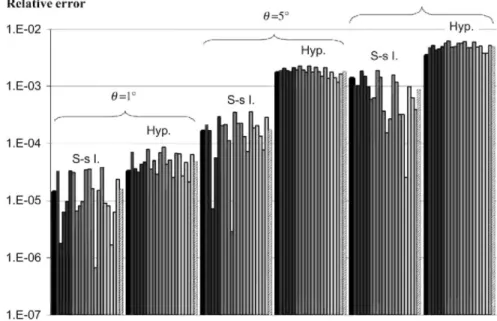
points are uniformly distributed in the domain. The mean error over these 21 points is also computed. The influence of the local approach: hyperplanes or stress-strain interpolation method is analyzed. The influence of the domain size [the angle θ defined by Eq. (18)] is also checked. The relative errors obtained are presented in Fig. 4.
A first remark concerning the computed errors is the large influence of the size of the domain: the mean relative error is almost multiplied by 100 if the size of the domain grows from 1° to 10°. Another important remark is the significant improvement of the accuracy of the stress-strain interpolation method compared to the hyperplane method. A factor around 10 between the mean relative errors of the two methods is observed when the larger local domains are tested (θ=5° and 10°).
It can also be noticed that the relative error strongly varies from one point to another with the stress-strain interpolation method while it is more uniform and exhibits a particular shape with the hyperplane method. Indeed, for the later method, the error is slightly lower at the center of the domain (dark gray points) and at the edges of the domain (light gray points) compared to other points in mid-gray. This can be explained by the fact that the error is smaller near the stress nodes (where the error is zero by definition) than far from them. Remember that one stress node is present at the center of the domain with the hyperplane method. This point clearly appears in Fig. 5.
Another remark not illustrated by Fig. 4 where the absolute values of the relative errors are indeed presented, is the fact that the hyperplane method always underestimates the yield stress. This point can also be clearly understood with Fig. 5 and is due to the convexity of the actual yield locus.
Fig. 3. Points where the relative error between the Taylor theory and the stress-strain interpolation method is
Fig. 4. Relative error between the Taylor theory and other models; 'S-s I' = the stress-strain interpolation
method, 'Hyp.' = the improved hyperplanes method, hatched cell ( ) = mean relative error.
Fig. 5. Bi-dimensional representation of the improved hyperplanes method.
4.2. Non radial loading strain paths
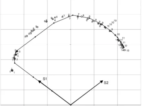
Complex loading paths are applied to the stress-strain interpolation method outside the finite element code to test the algorithm of local domain updating. The first complex path is a loading by tensile strain along the X-axis followed by a tensile strain along the Y-axis. The stress evolution computed by the constitutive law is plotted in Fig. 6 (the black points linked by straight lines) where the π-section of the yield locus is examined (S1 and S2 are
the two first principal stresses). For the present computations, the hardening is eliminated; the size of the local domains is θ=8°.
At the beginning of the X-axis tensile test, an increasing elastic stress state is observed. Then, when the yield stress is reached, the plasticity occurs. During the present computations, the total strain rate is imposed while the yield locus is plotted in stress space. As a consequence, due to the anisotropy of the yield locus, the stress state evolves on the yield locus during plastic deformations.
When the Y-axis tensile test is applied, an elastic unloading occurs followed by a reloading on another zone on the yield locus. Here again, the stress state evolves on the yield locus to accommodate the plastic deformations. In Fig. 6, the stress nodes corresponding to the successive local domains are also plotted (the symbols with a number). The numbers indicate the order into which the local domains defined by the corresponding stress nodes are computed. For instance, the five stress nodes constituting the fifth domain can clearly be visualized in Fig. 6. When it is possible, the updating of a local domain is achieved with the use of the adjacent domain as presented in Section 3.5. For instance, the number 4 only appears once in the graph. This means that the fourth domain explored is adjacent to the third one. When one number appears twice, three or four times, it means that two, three or four successive adjacent domains are explored before a satisfactory one is found.
Fig. 7 presents another complex loading path: the X-axis tensile test is now followed by shearing. The π-section of the yield locus is also examined for the visualization of the stress state evolution. Only a small part of the
yield locus including tension and shear is plotted in Fig. 7. An equivalent behavior of the model is observed. With the local yield locus approach, the representation of the yield locus is based on the stress nodes. In Fig. 7, it seems however that the stress state evolves outside the limit defined by the stress nodes. This effect is due to the projection of the stress nodes in the π-section which reduces their apparent amplitude. When the computed stress is closer to the π-section; its amplitude is less influenced by the projection.
Fig. 6. Successive tensile tests along rolling and transverse directions; black line = stress state, identical
symbols = stress nodes of one local domain, number = succession of the local domains.
Fig. 7. Tensile test in rolling direction followed by plane shear test; black line = stress state, identical symbols =
5. Deep drawing application 5.1. Cup drawing test
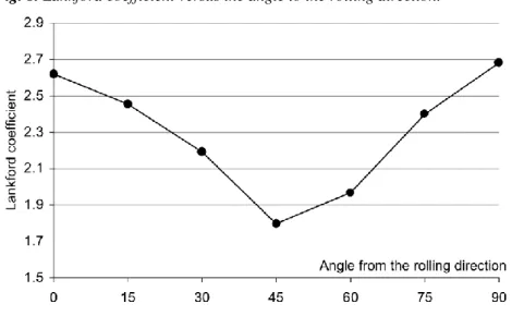
One of the deep drawing tests presented by Li et al. (2001) was chosen. It has been performed on a hydraulic press with a blank diameter of 100 mm, a punch diameter of 50 mm, a punch fillet of 5 mm, a die opening of 52.5 mm and a die fillet radius of 10 mm. A blankholder force of 5 kN was applied and the Coulomb friction coefficient was measured µ=0.05. An interstitial-free (IF) steel sheet of 0.84 mm thickness has been used. Its texture has been measured at mid-thickness and shows a strong γ fibre typical of rolled steel sheet. The maximum value of the ODF is 12.7. Fig. 8 presents the values of the Lankford coefficient computed from this texture by MTM-FHM software (Van Houtte, 1994b).
The hardening behavior has been measured by a tensile test along the rolling direction. The fitted hardening parameters of Eq. (16) are K=574 Mpa, ε0=0.00626 and n=0.326. Values of 210000 Mpa and 0.3 for the Young
modulus and the Poisson ratio are respectively employed in FE simulations. The earing profile, i.e. cup height as a function of the angle to Rolling Direction is manually measured at an interval of 15° and averaged over the symmetrically equivalent positions.
Fig. 8. Lankford coefficient versus the angle to the rolling direction.
5.2. FE simulations 5.2.1. Mesh description
LAGAMINE, the implicit Lagrangian FE code developed by the M&S department has been used. As in Li et al. (2001), the blank is meshed by one layer of linear brick finite elements. The BLZ3D brick finite element with eight nodes and one integration point developed by Zhu and Cescotto (1996) is chosen. This element is based on a mixed formulation in stress and strain with anti-hourglass stresses. Contact elements model the contact of the blank with the tools. The used CFI3D contact elements (Habraken and Cescotto, 1998) consist in plane elements defined by four nodes, four integration points. They are based on a penalty formulation. These contact elements are meshed on the surface of the blank using the same nodes as the ones defined for the blank. The tools are assumed to be rigid and meshed by triangular facets. Considering the orthortropic sample symmetry and the axisymmetry of the tools, only one quarter of the blank and of the tools are simulated in the FE model as shown in Fig. 9.
Fig. 9. Meshes of the blank and of the three tools.
5.2.2. Constitutive laws
In contact elements, the Coulomb friction law (Charlier and Cescotto, 1988) is used with a friction coefficient of 0.05. The penalty coefficients are 1000 N/mm3 between the blank and the matrix and 500 N/mm3 between the blank and the punch and the blankholder.
For comparison purposes, four different constitutive laws are used in the BLZ3D element: • 'Hill': the classical Hill (1948) constitutive law. The yield locus is defined by:
with σy the plastic stress measured in the rolling direction. The material parameters are fitted on the Lankford
coefficients shown in Fig. 8. Their values are F=0.5395, G=0.5526, H=1.4474, N=L=M=2.5091.
• 'Ani3vh': the sixth order series yield locus in stress space shortly described in Section 2.2. This yield locus has been identified outside the FE code, by 70 300 stress points computed by the Taylor theory applied on the initial texture.
and the 24 slip systems of a b.c.c metals are used (see Section 3.1). The texture is not updated and the initial texture converted by ODFLAM (Van Houtte, 2002) into a representative set of 2000 crystals is used throughout the simulation.
• 'Evol': identical to the 'Minty' law, but now the texture is updated every 10 time steps during the simulation. The micro-macro model without any analytical macroscopic yield locus implemented in LAGAMINE implicit code has never converged. In this case, at each integration point, the response of 2000 crystals was computed by the Taylor modules from Sections 3.1 and 3.2. So, result comparisons cannot be provided with this type of model, however computation time estimation will be analyzed in Section 5.2.4.
5.2.3. FE earing prediction analysis
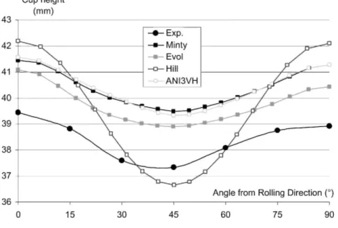
In a circular cup drawing operation, the prediction of the punch force and of the principal strains are less sensitive on the anisotropic constitutive law than the earing profile. So in Fig. 10, the earing behavior computed by the four anisotropic plastic laws is compared with the experiment.
The earing prediction shape provided by the 'Minty' law is close to the experimental one. A average shift of 1.92 mm can be noticed, compared to the experimental mean cup height of 38.42 mm. The predicted cup height is too high, meaning that the blank is retained too much between the blankholder and the matrix. A lower blankholder force or a lower friction coefficient would then improve the earing prediction. The finite element type has also a key influence, as only one layer of brick elements has been used. The bending stiffness of the element strongly affects the cup height. This is confirmed by Fig. 11 showing (for the Hill law) the results provided by two different brick elements of LAGAMINE code: BLZ3D (Zhu and Cescotto, 1996) and JET3D (Li et al., 1992). The curve computed by Li et al. (2001) with ABAQUS and the Hill law is also provided. Here not only a distinct element can explain the different earing behavior but also the other implementation of the Hill plasticity and the other contact model.
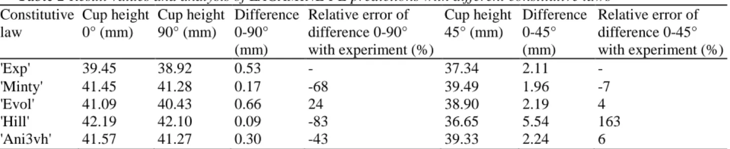
In Fig. 10, the constitutive law influence is clearly identified. One can notice that the prediction shift compared with experiment is reduced by updating the texture during the simulation (the 'Evol' law). The average shift is indeed of 1.27 mm for the 'Evol' case and of 1.92 mm for the 'Minty' case. However the 'Evol' law also brings an improvement in the predicted shape of the earing profile. Looking at the curve non-symmetry, or the minimum depth, the 'Evol’ result is closer to the experimental measures as quantified by Table 2. As underlined by this table, the Hill (1948) law results in a poor prediction of the shape and of the cup height. Note that LAGAMINE code automatically adapts its time step size to the equilibrium convergence speed and with 1045 time steps; it is the 'Hill' law that allows the larger time step size.
Fig. 10. Comparison of predictions by different constitutive laws and measured cup height versus the angle to
Fig. 11. Comparison of predictions by different finite elements and measured cup height versus the angle to the
rolling direction.
Table 2 Result values and analysis of LAGAMINE FE predictions with different constitutive laws
Constitutive law Cup height 0° (mm) Cup height 90° (mm) Difference 0-90° (mm) Relative error of difference 0-90° with experiment (%) Cup height 45° (mm) Difference 0-45° (mm) Relative error of difference 0-45° with experiment (%) 'Exp' 39.45 38.92 0.53 - 37.34 2.11 - 'Minty' 41.45 41.28 0.17 -68 39.49 1.96 -7 'Evol' 41.09 40.43 0.66 24 38.90 2.19 4 'Hill' 42.19 42.10 0.09 -83 36.65 5.54 163 'Ani3vh' 41.57 41.27 0.30 -43 39.33 2.24 6
According Table 2, the "Ani3vh" law provides accurate results: better than the "Minty" law but worse than the "Evol" law. However, Table 2 analysis is quite refined and the above conclusion should be taken with caution. As both laws 'Minty' and 'Ani3vh' rely on identical initial texture and micro-macro Taylor model, one should expect that they provide quite identical results, which is nearly confirmed by Fig. 10. The 'Ani3vh' law works with an analytical yield locus with normality rule and the FE simulation is performed within 1861 time steps. This yield locus averages more the response of the representative crystals than the local yield locus proposed by the 'Minty' law. With this law, the FE simulation requires 1741 time steps. So one cannot tell if the 'Minty' law is less efficient than a classical law with normality rule. For materials where the sixth order yield locus is close to the actual yield locus, the 'Minty' law does not improve accuracy. However the better performance of the 'Evol' law demonstrates the interest of the local description of the yield locus. It takes into account the heterogeneous evolution of the anisotropy. A second point is the fact that texture intensity increases during deep drawing process and should be less accurately represented by a sixth order yield locus. Note that near the top of the cup, the maximum texture intensity in the rolling, 45° and transverse directions predicted by the Taylor theory are respectively 58, 52, and 49.
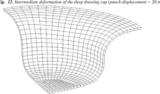
A typical configuration happening during this deep drawing process is chosen. It corresponds to a punch travel of 20 mm (see Fig. 12). For this deformation state, Figs. 13-15 plot the principal strains against curvilinear abscissa respectively along the rolling direction, the 45° direction and the transverse direction. As shown in Fig. 13, five zones can clearly be distinguished on the cup:
• The first zone is the part of the steel sheet, which stays under the punch until the end of the deep drawing process. The maximum principal strains in the plane of the sheet (E1 and E2 in Figs. 13-15) are relatively small in this zone, while large displacements take place. Indeed, the steel sheet follows the punch travel without large deformation. An equi-biaxial tension state or stretched zone is present (E1 ≈ E2). The thickness strain (E3) is negative, corresponding to a thickness reduction.
• The second zone is the part of the steel sheet applied against the shoulder of the punch. The strain state corresponds to stretching, but with E1 larger than E2.
Indeed, a maximum in E1 and E3 (in absolute value) is reported numerically. This maximum is created at the beginning of the deep drawing simulation, when the steel sheet in contact with the curved part of the punch is highly stretched due to the effect of the blankholder. After that moment, the strains in this second zone remain constant.
• The third zone is the flange of the cup. The maximum principal strain increases in this zone as curvilinear abscissa s increases, while the minimum principal strain decreases and is negative. The thickness strain is also negative but almost constant. This zone is a restrained zone, typical of deep drawing processes (E1 > 0 and E2 < 0).
• The fourth zone corresponds to the steel sheet applied against the shoulder of the matrix. In this zone, the restrained state is maximum and the thickness strain becomes positive, so the sheet thickness increases. • The fifth zone is the part of the steel sheet under the blankholder during the deep drawing process. After the maximum of the fourth zone, the restrained strain state decreases in the fifth zone, as the contact with the matrix and the blankholder reduces the tension of the sheet. The second principal strain (E2) is a compression strain and becomes larger than the tensile strain E1 (E1 > 0, E2 < 0 and ||E1|| < ||E2||). The compression strain would give rise to instability and wrinkling without the action of the blankholder. It results in an increase of the sheet thickness.
For this test, no strain measurements were available, however for other deep drawing tests (Duchêne et al., 1999, 2002; Duchêne, 2002) strain measurements have been performed and confirm the type of predictions plotted in Figs. 13-15. These curves verify that the different constitutive laws do not strongly affect the strain distribution. However the integration of these strains provides noticeable differences in the earing profile.
In zone three, the cup flange, the tensile principal strain E1 is predominant: E1 > 0 and E2 < 0 with ||E1|| > ||E2||. The strain repartition depends of course on the punch radius and material anisotropy. However, E1 strain is mainly induced by the punch displacement and the phenomena happening in zone five. One can mainly link the earing profile to the mechanical state of zone five and the Lankford coefficient. The fifth zone is very large at the process beginning and decreases as the process goes on. Under the blankholder, the compression strain is predominant: E1 > 0 and E2 < 0 with ||E1|| < ||E2|| (see Figs. 13-15). So, the thickness tends to increase (E3 > 0) and this effect is more pronounced where the r value is small. Due to the conservation of the volume during plastic deformations, where the thickness is the larger, the radial strain is more important. This explains the observed minimum in Fig. 10 around 45° direction where the Lankford coefficient (Fig. 8) is minimum.
Fig. 13. Principal strains along the rolling direction.
Fig. 14. Principal strains along the 45° direction.
The strain states along the different directions in zone five are analyzed in the top of Fig. 16. Considering a point along the rolling direction, the compression strain is acting along a circumferential direction, which coincides with the transverse direction for this point. Similarly, along the transverse direction, the compression direction is the rolling direction and for the 45° direction; it is the direction at 45° from the rolling direction. The consequences on the earing profile are presented in the bottom of Fig. 16.
Analyzing Fig. 8 and Table 2, one can verify that the behavior predicted by Fig. 16 follows both experimental and numerical results:
This approach has been verified for other experiments as described in Duchêne (2002). This strong link of the earing behavior with the Lankford coefficient also explains why the 'Evol' law increases prediction accuracy. Texture updating modifies the Lankford coefficients in the flange, which affects the earing prediction.
Fig. 16. Strains happening under the blankholder and link between the earing profile and the Lankford
coefficient.
5.2.4. CPU time analysis
The expected reduction of the computation time by the stress-strain interpolation method can be estimated by analyzing the number of activations of the micro-macro Taylor module (described in Section 3.2). The influence of the texture evolution on this number can also be analyzed. Table 3 provides the number of activations of different modules during the FE cup drawing simulations.
Table 3 Analysis of module activations
Constitutive law Number of activations of the Micro-macro Taylor module
Yield locus exploration Constitutive law
'Minty' 475539 75202434 3692574
'Evol' 1944712 120603774 5961006
For the 'Minty' or 'Evol' cases, the number of activations of the constitutive law is the total number of global equilibrium iterations during the FE computation multiplied by the number of BLZ3D elements (531 for this example). Remember that LAGAMINE code automatically adapts its time step size to the equilibrium
step size. With the 'Evol' law, the yield locus follows the anisotropy evolution and it slows down the convergence (61% more iterations).
If the constitutive law is activated Y times, the iteration scheme described in Fig. 1 is called ( Y multiplied by the number of sub-steps) times. The number of substeps is adjusted on the strain increment size for each integration point and during the whole simulation. In the developed integration scheme, the yield locus exploration happens either to detect plastic state or to find the strain rate direction uB associated to the stress sB. So, the number of
yield locus explorations depends on the convergence of the stress integration scheme. Without the stress-strain interpolation method the micro-macro Taylor module should be activated at each yield locus exploration. With the 'Minty' law, the micro-macro Taylor module is called only once for about 158 yield locus explorations (75, 202, 434/475, 539). When the texture is not updated, this factor estimates the gain of the stress-strain
interpolation method compared to the micro-macro models of Section 2.1 without analytical macroscopic yield locus. One could argue that this estimation is false because linked to the developed integration scheme. However, forgetting this scheme, the numbers just reveal: 20 yield locus explorations for each activation of the constitutive law. This is not excessive, knowing the frequent use of sub-steps and the required iterations to identify the elastic and plastic parts of the step.
For the 'Evol' law, the user imposes a texture updating every 10 time steps. As 2712 time steps were performed and there were 531 interpolation points or elements, micro-macro Taylor module has been activated 143901 (271 multiplied by 531) for texture updating. When the texture is modified, five new stress nodes have to be
computed, which means 719505 activations of the micro-macro Taylor module (143 901 multiplied by 5). Finally, 863406 (143901+719505) activations or 44% are directly linked to the texture updating, the other 56% can be explained as in the 'Minty' case. Globally, in the 'Evol' law, micro-macro Taylor module is activated once for 62 yield locus explorations (120, 603, 774/1, 944, 712). The gain of stress-strain interpolation method compared to models of Section 2.1 is lower if the texture evolution is required.
The simulations have been achieved on a SGI Origin3800 computer equipped by 60 processors. Other members of the M&S team (Moto Mpong et al., 2002; de Montleau et al., 2002) have developed a parallel processing of LAGAMINE code. Observing that with the 'Minty' or 'Evol' laws, more than 90% of the computation time is spent in the constitutive laws, Open MP protocol has been applied to parallelize the element loop between the available processors. The direct solver has also been adapted to multiprocessing (Cela, 2001). Hereafter, the given simulation times mean the sum of the computation time of each processor:
'Hill' = 44 min 'Minty' = 29 h 'Ani3vh' = 123 min 'Evol' = 130 h
Compared to a global analytical yield locus model, like the 'Ani3vh' law, the stress-strain interpolation method without texture updating (the 'Minty' law) induces a large increase of CPU time. This is not surprising as no micro-macro computation happens during the simulation with the 'Ani3vh' law. If the anisotropy is well
described by a sixth order series yield locus and that texture updating is not important, the 'Ani3vh' law improves the accuracy compared to the 'Hill' model and keeps reasonable CPU time.
6. Conclusions
The stress-strain interpolation method has been described. Coupled with a micro-macro Taylor model, its accuracy has been verified for different strain paths and one deep drawing process. Additional validations on experimental deep drawing processes can be found in Duchêne et al. (2002) and Duchêne (2002).
This new method follows the yield stresses predicted by the Taylor theory more closely than a global sixth order series yield locus (the 'Ani3vh' law) adjusted on stresses computed by the Taylor model for the initial texture. The stresses computed by the stress-strain interpolation method stay very close to the stresses computed by the micro-macro Taylor module, since they are strictly imposed on the domain limit vectors defining the
interpolation domain. In case of texture evolution, the advantage of FE simulations with the 'Evol' law has been confirmed. When texture evolution is neglected, the advantage of the 'Minty' law compared with the 'Ani3vh' law does not clearly appear. The accuracy of the sixth order series yield locus proposed by the 'Ani3vh' law is sufficient. It will be investigated if the answer is identical for very strong textures or other crystal lattices known to provide non-smooth yield loci.
The important problem of multiple normals at the boundary of two neighbor local descriptions has been solved; it is a key point with local yield locus description. As explained, the stress-strain interpolation method does not impose the normality rule strictly. Specific and robust integration scheme of this new constitutive law has been developed. The comparison of the number of time steps between FE simulations with 'Ani3vh' or 'Minty' laws confirms the efficiency of the new approach.
Section 5.2.4 quantifies the decrease of the number of activations of the micro-macro module by the stress-strain interpolation law compared to a classical micro-macro method averaging crystal stresses. Factors of 158 and 62 are respectively associated to models without or with texture updating. As the advantage of the method has been established with a micro-macro model of Taylor type, next step is to couple the method with other micro-macro models that are known to be more accurate and greedier from a CPU time point of view. For instance, the multisite approach of Delanny et al. (2002) will be soon coupled with the stress-strain interpolation method. The stress-strain interpolation method is not limited to f.c.c or b.c.c. metals. Any material, which can be described by a macroscopic elasto-plastic behavior, can be modeled as long as an adapted micro-macro model exists.
Simple isotropic hardening is not satisfactory and the 'Minty' law is currently extended to the kinematic hardening model proposed by Bouvier et al. (2003). One next step will be the use of Mandel spin to follow the rotation of the material axes. The advantage of this modification has been checked by Peeters et al. (2001). Thanks to the efficient method proposed by Van Houtte (2001) to compute Mandel spins for all possible strain modes, this should be compatible with FE simulations.
Acknowledgements
As Senior Research Associate of National Fund for Scientific Research (Belgium), Anne Marie Habraken wishes to acknowledge support of the Belgian research fund. The team of Paul Van Houtte is acknowledged for the possibility of using their texture modules and providing the deep drawing experiment data. The authors also thank the Belgian Federal Science Policy Office (Contract P5/08) for its financial support.
References
Aifantis, E.C., 1987. The physics of plastic deformations. Int. J. Plasticity 3, 211-247.
Anand, L., Kothari, M., 1996. A computational procedure for rate independent crystal plasticity. J. Mech. Phys. Solids 44 (4), 525-558. Anand, L., Balasubramanian S., Kothari, M., 1997. Constitutive modeling of polycrystalline metals at large strains: application to
deformation processing, large plastic deformation of crystalline aggregates. In: Teodosiu (Ed.), International Centre for Mechanical Sciences, CISM Courses and Lectures 376. Springer, pp. 109-172.
Arminjon, M., Bacroix, B., Imbault, D., Raphanel, J.K., 1994. A fourth-order plastic potential for anisotropic metals and its analytical calculation from texture function. Acta Mechanica 107, 33-51.
Asaro, R.J., Needleman, A., 1985. Texture development and strain hardening in rate dependent polycrystals. Acta Metallurgica 33, 923-953.
Beaudoin, A.J., Dawson, P.R., Mathur, K.K., Kocks, U.F., Korzekwa, D.A., 1994. Application of polycrystal plasticity to sheet forming. Comp. Methods Appl. Mech. Eng. 117, 49-70.
Beaudoin, A.J., Dawson, P.R., Mathur, K.K., Kocks, U.F., 1995. A hybrid finite element formulation for polycrystal plasticity with consideration of macrostructural and microstructural linking. Int. J. Plasticity 11 (5), 501-521.
Berveiller, M., Zaoui, A., 1978. An extension of the self-consistent scheme to plastically-flowing polycrystals, J. Mech. Phys. Solids 26 (5-6), 325-344.
Bouvier, S., Teodosiu, C, Haddadi, H., Tabacaru, V., 2003. Anisotropic work-hardening behaviour of structural steels and aluminum alloys at large strains. J. Phys IV France 105, 215-222.
Cela, J.M., 2001. Library CAESAR. Centro Europeo de Paralelismo de Barcelona, Barcelona.
Charlier, R., Cescotto, S., 1988. Modélisation du phénomène de contact unilatéral avec frottement dans un contexte de grande déformation (special issue). J. Theoret. Appl. Mech., 7(Suppl. 1).
Chastel, Y., Loge, R., Perrin, M., Lamy, V., Zaefferer, S., 1998. Microscopic and macroscopic length scales in hot extrusion of Zircaloy 4. In: Chenot, J.L., Agassant, J.F., Montmitonnet, P., Vergnes, B., Billon, N., (Eds.), Proceedings of the First ESAFORM Conference on Material Forming (CEMEF CNRS UMR 7635), p. 37.
Crumbach, M., Pomana, G., Wagner, P., Gottstein, G. 2001a. A Taylor type deformation texture model considering grain interaction and material properties. Part I - fundamentals. In: Gottstein G., Molodov D.A., (Eds), Recrystallization and Grain Growth, Proc. of the First Joint Int. Conf. Springer-Verlag.
Crumbach, M., Pomana, G., Wagner, P., Gottstein, G. 2001b. A Taylor type deformation texture model considering grain interaction and material properties. Part II - experimental validation and coupling to FEM. In: Gottstein G., Molodov D.A., (Eds), Recrystallization and Grain Growth, Proc. First Joint Int. Conf. Springer-Verlag.
Darrieulat, M., Piot, D., 1996. A method of generating analytical yield surfaces of crystalline materials. Int. J. Plasticity 12 (10), 1221-1240. Darrieulat, M., Montheillet, F., 2003. A texture based continuum approach for predicting the plastic behavior of rolled sheet. Int. J. Plasticity 19 (4), 517-546.
Delanny, L., Kalidindi, S.R., Van Houtte, P., 2002. Prediction of intergranular strains in cubic metals using a multisite elastic-plastic model. Acta Mater. 50, 5127-5138.