HAL Id: hal-01685374
https://hal.archives-ouvertes.fr/hal-01685374
Submitted on 16 Jan 2018
HAL is a multi-disciplinary open access
archive for the deposit and dissemination of sci-entific research documents, whether they are pub-lished or not. The documents may come from teaching and research institutions in France or
L’archive ouverte pluridisciplinaire HAL, est destinée au dépôt et à la diffusion de documents scientifiques de niveau recherche, publiés ou non, émanant des établissements d’enseignement et de recherche français ou étrangers, des laboratoires
Energetic approach for a sliding inclusion accounting for
plastic dissipation at the interface, application to phase
nucleation
Joffrey Bluthé, Daniel Weisz-Patrault, Alain Ehrlacher
To cite this version:
Joffrey Bluthé, Daniel Weisz-Patrault, Alain Ehrlacher. Energetic approach for a sliding inclusion accounting for plastic dissipation at the interface, application to phase nucleation. International Journal of Solids and Structures, Elsevier, 2017, 121, pp.163-173. �10.1016/j.ijsolstr.2017.05.023�. �hal-01685374�
Energetic approach for a sliding inclusion accounting for plastic
dissipation at the interface, application to phase nucleation.
Joffrey Bluthéa, Daniel Weisz-Patraultb, Alain Ehrlachera
aLaboratoire Navier, CNRS, École des Ponts ParisTech, 6 & 8 Ave Blaise Pascal, 77455 Marne La Vallee, France bLMS, École Polytechnique, CNRS, Université Paris-Saclay, 91128 Palaiseau, France
Abstract
The energy gained at the atomic scale by modifying the crystal lattice during phase nu-cleation is an important aspect to study solid-solid phase transitions. However at the scale of continuum mechanics, the eigenstrain introduced by the geometrical transformation in the newly formed phase is also a significant issue. Indeed, it is responsible for very large elastic energy and dissipation that have to be added to the total energy in order to determine if a phase transition can occur. The eigenstrain can cause sliding of the newly formed grain. In this paper, an analytical solution coupled with numerical energetic optimization is derived to solve the problem of a two-dimensional circular elastic sliding inclusion authorizing plastic dissipation at the interface. Numerical calculations under plane stress assumption show that dissipation enables an effective decrease in the energy needed for the phase transformation to occur. The solution is validated with a comparison with a Finite Element simulation.
Keywords:
Phase transition; Plastic dissipation; Elastic energy; Energetic approach; Sliding inclusion; Eigenstrain
1. Introduction
Phase transitions are crucial for many applications. A general strategy for modeling phase transitions consists in constructing a cost function (or a global energy) by adding different energetic contributions and dissipated energies arising at different scale during phase transition. Then a minimization over possible states (i.e., a global energy balance) is considered in order to determine if phase nucleation is the most favorable option with respect to the energetic cost function as proposed for instance by Fischer and Reisner (1998).
Among the energetic contributions that should be considered, one of the most studied is the energy gain by the rearrangement of the crystal lattice Müller et al. (2007). This contribution is associated to the free Gibbs energy variation between one phase and the other. However, the geometrical transformation from the crystalline structure of the parent phase to the crys-talline structure of the product phase, amounts to impose, at the scale of continuum mechanics, an eigenstrain in the product phase. For instance within the framework of steel well known orientation models proposed by Bain and Dunkirk (1924); Nishiyama (1934); Kurdjumow and Sachs (1930) may be used to quantify this eigenstrain.
Thus, the free Gibbs energy variation between the parent phase and the product phase is not sufficient to evaluate if phase transformation may occur. Indeed, at the scale of continuum mechanics, the newly formed phase nucleates with a certain size. The geometrical transfor-mation undergone in the inclusion is thus incompatible with the presence of the surrounding matrix, and the inclusion and the matrix will therefore experience elastic strains. Phase nucle-ation occurs if a lower total energy is reached. Therefore, this elastic energy tends to reduce the possibility of phase changes because the energy gained at the atomic scale by the modifi-cation of the crystal structure is compensated by the bulk energy at a larger scale. Thus, one needs to evaluate the elastic energy associated with the eigenstrain in order to correctly predict phase nucleation. For instance, within the framework of Zirconium phase transition, Hensl et al. (2015) include elastic energy in the global free Gibbs energy. Usually the well-known in-clusion method proposed by Eshelby (1957) is used to evaluate the stored elastic energy due to the eigenstrain. For instance Lambert-Perlade et al. (2004) used the Eshelby inclusion method to model self-accommodation within the framework of austenite to bainite phase transition in steel alloys. Mura et al. (1976) proposed an extension of the Eshelby inclusion method for anisotropic materials and consider applications to martensite formation. Previous works con-sider purely elastic materials even though non-negligible plastic strain may occur. Thus, Delan-nay et al. (2008) proposed to evaluate elastic-plastic accommodation by using a Finite Element model of an embedded-cell model. One can also mention a different strategy proposed by Am-mar et al. (2009) based on a phase-field model of phase transition in elastic-plastic materials where the free energy density accounts for dissipation and elastic and chemical1contributions.
All the previously mentioned works are based on a perfect adhesion between the inclusion and the surrounding matrix of the parent phase. However, experimental evidences of sliding inclusions have been published by Saotome and Iguchi (1987) for instance. Thus, this pa-per aims at developing an alternative inclusion method adapted to sliding inclusions and that takes into account plastic dissipation at the interface. The significance of sliding inclusions on the elastic energy when considering phase transitions was already investigated by Tsuchida et al. (1986) and Mura et al. (1985); Jasiuk et al. (1987) for perfectly sliding inclusions in two and three dimensions respectively. More precisely, continuity of normal traction and normal displacements at the inclusion/matrix interface is verified as well as a condition of vanishing shear traction. Tangential displacements are discontinuous at the interface and are determined through the latter shear free condition. On this basis, it was shown that allowing for sliding reduces the energy needed for the transformation to occur. In this paper, imperfectly sliding inclusions are considered and shear stresses are not set to zero at the interface.
Imperfectly sliding inclusions have already been solved by Huang et al. (1993) and Ru (1998), by modeling the relative magnitude of sliding by introducing a parameter varying be-tween zero (perfectly bounded interface) and one (perfectly sliding interface) and by Zhong and Meguid (1997) by assuming that the normal stress is proportional to the corresponding tan-gential displacement discontinuity which amounts to a Coulomb type friction law. Relying on the same assumption, Mogilevskaya and Crouch (2002) solved the problem of multiple circular sliding inclusions by using a Galerkin boundary integral method.
The approach developed in this paper differs from previous solutions to the extent that there is no assumption on shear traction at the interface and no a priori relationship between tangential displacement discontinuity and normal traction. The problem of an inclusion subject to a known eigenstrain and prescribed sliding is solved with continuity of normal and shear traction and continuity of normal displacement at the interface. The whole solution depends on the prescribed slip and energetic arguments are eventually used in order to determine the actual slip that the system will reach.
These energetic arguments come from experimental observations performed by Saotome and Iguchi (1987) that enable to interpret sliding as localized plasticity at the interface. There-fore, dissipated energy should be taken into account. This is not allowed by the previously mentioned papers, where sliding is determined by an arbitrary proportionality relation between
normal traction and tangential displacement discontinuity or by setting shear traction to zero. The energetic approach, that ultimately enables to determine sliding, classically consists in minimizing a global energy that takes into account bulk energy and plastic dissipation. Within the framework introduced for instance by Fedelich and Ehrlacher (1997) and Mielke (2003), dissipation can be seen as a cost (or a distance) that the system has to pay (or to cross) to get a new state, therefore the state variables are those that optimize the bulk energy accounting for the cost to reach this new state. It should be noted that plasticity is considered only at the interface (shear band) and not in the inclusion or matrix bodies.
In the present work, these ideas are applied to the two-dimensional problem of a circular inclusion subject to a given eigenstrain and surrounded by an infinite matrix. An approximate solution to the problem of an inclusion subject to a given eigenstrain and an arbitrary sliding prescribed at the interface is first derived in the context of complex analysis and the works of Muskhelishvili (1953). A numerical minimization of the sum of elastic and dissipated energies at the interface (given as a function of the prescribed sliding) is then performed, in order to determine the actual sliding that the system will reach when loaded by the eigenstrain. A yield strength for the boundary is introduced in order to compute the dissipated energy. This varia-tional method ensures that the von Mises yield criterion is met for sliding to occur. Numerical calculations show that for small eigenstrains, the yield criterion has a very simple interpreta-tion: the absolute value of the tangential component of the interfacial tractions is equal to the yield strength where sliding occurs, and it is strictly below it where sliding does not occur. The numerical results thus obtained are then compared with results from a finite element method calculation performed on Abaqus in the case of free slip. Note that the general case of a finite yield strength would require the introduction of interface elements with a plastic behavior be-tween the inclusion and its surroundings, which does not appear to be implemented in Abaqus to the best of the authors’ knowledge. One contribution of this work is thus the ability of the method to deal with a perfectly plastic interface. Finally, the behavior of the solution pro-posed with finite yield strength is investigated. Three regimes are essentially found: when the eigenstrain is sufficiently low no slip occurs at the interface, then for a certain amplitude slip starts to occur locally and the tangential component of the interfacial tractions is found to be consistent with the yield criterion, and finally for large enough amplitude slip occurs on the whole interface so that the criterion is met at all of its points. The convergence of the results
with the truncation of the expansions is also investigated, and a Gibbs phenomenon is naturally observed when the tangential component becomes discontinuous.
The approximate solution developed here is eventually used to estimate the mechanical energy that has to be provided by the surroundings to the system for a single circular region of space to undergo a phase transition with a given eigenstrain. The plastic dissipation at the interface is shown to be non neglectable with respect to the elastic energy stored during the process. The total energy, that is the sum of the elastic energy and the plastic dissipation, is thus interpreted as the energy that is needed for this phase transition to occur locally.
2. Semi-analytical solution to the problem of a circular sliding inclusion with non-zero tangential component of the interfacial tractions
The semi-analytical solution to the problem of a sliding circular inclusion subject to a given uniform eigenstrain expressed in its principal directions is derived in this section:
ε∗= ε∗xx 0 0 ε∗yy (1)
Both the inclusion and the matrix are linear elastic and plane theory of elasticity is con-sidered. The Lamé coefficients of the inclusion and the matrix are denoted by (λI, µI) and (λM, µM), where I and M stand for inclusion and matrix respectively. The following derivation uses complex potentials and expansions into power series, Laurent series and Fourier series. The solution that is derived here can be broken down into three parts. First, the solution to the problem of a disk with prescribed surface tractions at the boundary, and the solution to the problem of a matrix with a circular hole with prescribed surface tractions along the hole and no displacement at infinity are addressed in sections 2.2 and 2.3 respectively. These solutions are obtained by expanding the prescribed surface tractions into a Fourier series and is quite analogous to the solutions given by Muskhelishvili (1953). Then, using these two preliminary solutions, the problem of a circular inclusion subject to a given uniform eigenstrain and a pre-scribed trial sliding along the interface is derived in section 2.4. The trial sliding is denoted by g(θ) where r, θ are polar coordinates. Eventually the actual sliding that the system will reach is denoted by gS(θ) where S stands for solution. To solve this sliding inclusion problem,
the prescribed surface tractions are eliminated using continuity conditions on the displacement (accounting for the trial sliding g(θ)) and the continuity of the normal and shear traction. As a result, displacements and stresses in the whole domain as a function of the prescribed trial slid-ing are obtained. At this point, it is necessary to point out that the interfacial tractions are not known during the first step, so it is natural that they should be eliminated at some point. Also, in the general case, it is not possible to derive the exact analytical solution to this problem, as an infinite number of equations are obtained with an infinite number of unknowns to eliminate. It is however possible to truncate the series and derive numerically efficient solutions obtained by simply inverting a matrix. Finally, the third step consists in using the solution to the prob-lem of the prescribed trial sliding g(θ) at the interface to numerically minimize the sum of the elastic potential energy and the plastic dissipation at the boundary. Thus the determination of the actual sliding that the system will reach reads:
gS(θ) = argmin g(θ)
E[g(θ)] (2)
where the global energy E[g(θ)]is written:
E[g(θ)]= WE [
g(θ)]+ D[g(θ)] (3) Where WE is the stored elastic energy and D the plastic dissipation. The elastic energy can be computed numerically by an integral on the interface and the plastic dissipation as well. It should be noted that the actual sliding gS(θ) is thus a result of the calculation, and the loading is obviously the eigenstrain in the inclusion. At each step of the minimization, a certain sliding is postulated and the resulting global energy accounting for plastic dissipation is computed. The algorithm searches for the sliding that minimizes the global energy, and to do that an expansion of the sliding g(θ) into a Fourier series is used so as to minimize on a finite number of parameters, namely the coefficients of the Fourier series.
As a result of the minimization process, E[gS(θ)]is obtained, which is the amount of en-ergy that has to be provided by the surroundings to the system during the process. Thus, it is interpreted as the energy needed for a phase transition to occur in a circular region of space, assuming that this phase transition prescribes an eigenstrain to the inclusion, such as that pre-scribed by the austenite-ferrite transition.
2.1. Preliminary remarks
A well known approach introduced by Muskhelishvili (1953) for plane isotropic elasticity under infinitesimal strain assumption is to use two holomorphic potentialsϕ(z) and ψ(z) that are complex functions of z = x + iy = reiθ, where x and y are the Cartesian coordinates (matching the principal directions of the given eigenstrain) and r andθ the polar coordinates. z is thus the position of the point under consideration in the complex plane. These potentials are defined so that one can derive from them the components of the stress tensor and of the displacement vector at any given point of the elastic body considered, using the following equations in the polar basis: σrr+ σθθ = 2(ϕ′(z)+ ϕ′(z)) σθθ− σrr+ 2iσrθ = 2e2iθ(zϕ′′(z)+ ψ′(z)) 2µ(ur+ iuθ) = e−iθ(κϕ(z) − zϕ′(z)− ψ(z)) (4)
whereµ is the shear modulus of the body and κ is defined by:
κ = λ + 3µλ + µ (5)
where λ is the Lamé’s first parameter of the body. One indeed uses λ if one deals with a plane strain problem, but in the case of plane stress, one needs to replaceλ by λ∗defined by:
λ∗= 2µλ
λ + 2µ (6)
It should be noted that potentials ϕ and ψ are not unique. Using the fact that they are holomorphic, Muskhelishvili (1953) shows that two pairs of potentialsϕ1,ψ1 andϕ2,ψ2 yield
the same state of stress if and only if one has: ϕ2(z) = ϕ1(z)+ Ciz + γ ψ2(z) = ψ1(z)+ γ′ (7)
where C is a real constant andγ and γ′are two complex constants. He also shows that they yield the same displacement if and only if one has:
C = 0 κγ − γ′ = 0 (8)
This is due to the fact that C determines the rigid body rotation and κγ − γ′the rigid body translation of the body. This should be considered to deal with rigid body motions of the inclusion and the matrix in order to be able to fit the two solutions correctly.
2.2. An inclusion subject to prescribed surface tractions at the matrix interface
Consider an elastic circular inclusion of radius R subject to prescribed surface tractions. Useful results for the present paper are exposed but calculations are not detailed since similar problems are solved by Muskhelishvili (1953). The potentials ϕ and ψ are holomorphic in a simply connected region, so they can be expanded into a power series:
ϕ(z) = +∞∑ k=0ϕk
zk and ψ(z) = +∞∑ k=0ψk
zk (9)
The surface traction is written as a simple complex function, namelyσI
rr(R, θ) − iσrIθ(R, θ) (with a superscript I for inclusion), that is expanded into a Fourier series:
σI rr(R, θ) − iσ I rθ(R, θ) = N−1 ∑ k=−N+1 Dkeikθ (10)
where Dk are the Fourier coefficients of the tractions. At this stage, only the expansion of the tractions is truncated, however identification of the coefficients shows that the holomorphic potentials have a finite number of non-zero coefficients, that are given by:
D1 = 0 ϕ1+ ϕ1 = D0 ∈ R ϕn = R 1−n n D1−n, 2 ≤ n ≤ N ψn = −R 1−n n (Dn+1+ nD−(n+1)), 1 ≤ n ≤ N − 2 (11)
It should be noted that D1 = 0 and D0 ∈ R are equivalent to the resultant force and
mo-ment acting on the inclusion vanishing, namely to the global equilibrium of the inclusion. At this point,ϕ0,ψ0and the imaginary part of ϕ1 are undetermined, which is consistent with the
remarks of 2.1 since the rigid body motion of the inclusion is unknown. Introducing the elastic constants of the inclusionκIandµI, one can deduce the displacement uI at the boundary r= R after straightforward calculations:
2µI(uIx− iuIy) = − −3 ∑ k=−N κI kDk+1Re ikθ +κI 2D−1Re−2iθ+ ( κI−1
2 D0R− i(κI+ 1)ℑ(ϕ1))e−iθ
+κIϕ0− ψ0− D−1R+ N∑−2 k=1 1 kDk+1Re ikθ (12)
whereℑ(z) denotes the imaginary part of z.
2.3. A matrix subject to prescribed surface tractions at the inclusion interface
Consider an infinite elastic matrix with a circular hole of radius R subject to prescribed surface tractions at the inclusion interface. Alike the previous problem only the useful results for the present paper are exposed. One proceeds in the same fashion as in the case of the inclusion, except that this time the domain is not simply connected, so that the potentials, denoted hereα(z) and β(z), have to be expanded into a Laurent series. It is assumed that there are no displacements at infinity, so that the matrix does not have any rigid body motion. Thus the expansions ofα(z) and β(z) do not possess any term with a positive exponent. The angular position of the point under consideration will be denotedφ instead of θ to avoid confusion later:
α(z) =∑+∞ k=0 αk zk and β(z) = +∞ ∑ k=0 βk zk (13)
The surface traction is written as a simple complex function that is expanded into a Fourier series as was previously done, but the coefficients will be denoted Pk instead of Dk:
σM rr(R, φ) − iσ M rθ(R, φ) = N−1 ∑ k=−N+1 Pkeikφ (14)
As previously, one automatically gets P1= 0, however one does not get P0 ∈ R. This is due
to the fact that a non-zero resultant moment on the boundary of the hole can be in equilibrium with stresses at infinity. Basic calculations give:
αn = −R n+1 n Pn+1, 1 ≤ n ≤ N − 2 β1 = R2P0 β2 = R 3 2 P−1 βn = R n+1 n (P1−n− nPn−1), 3 ≤ n ≤ N (15)
and it is obtained again thatα0andβ0are undetermined, but the condition of zero
displace-ment at infinity gives the following condition:
κMα0− β0= 0 (16)
whereκM is one of the elastic constants of the matrix. Introducing the second elastic con-stants of the matrixµM, one can deduce the displacement uM at the boundary r= R:
2µM(uMx − iu M y )= −3 ∑ k=−N 1 kPk+1Re ikφ− 1 2P−1Re −2iφ− P 0Re−iφ− N−2 ∑ k=1 κM k Pk+1Re ikφ (17)
2.4. Problem of the inclusion with given eigenstrain and prescribed sliding
The results obtained previously are now used to solve the problem of an inclusion subject to a given eigenstrain and prescribed sliding g(θ) with respect to the surrounding matrix. For usual non sliding inclusion problems, the interfacial tractions are determined by displacement and traction continuity. The problem being solved here considers a prescribed sliding, and the identification of the interfacial tractions cannot rely on displacement continuity but on matching positions after transformation. The sliding is defined as follows. At the interface, consider a material point belonging to the inclusion located by the angular position θ, a material point belonging to the matrix is then selected and located by the angular position φ(θ) so that after transformation both material points coincide. The sliding is then defined by the quantity:
g(θ) = φ(θ) − θ (18)
It should be noted that the interfacial tractions implicitly depend on the prescribed sliding
points defined by Reiφ(θ)in the matrix, consider first u∗the displacement due to the eigenstrain ε∗alone as though the inclusion could expand freely, namely u∗= ε∗.XI (where XIdenotes the position of a material point in the inclusion). Then, consider uIand uMthe displacements of the inclusion and the matrix respectively due to the interfacial tractions arising from the interaction between the inclusion and the matrix, namely the solutions obtained in sections 2.2 and 2.3. Thus the coinciding condition reads:
Reiθ+ u∗x+ iu∗y+ uIx+ iuyI = Reiφ(θ)+ uMx + iuyM (19) Only infinitesimal sliding will be considered in what follows, that is g(θ) << 1. Note that a given uniform finite sliding g(θ) = g0is compatible with zero strains in both the inclusion and
the matrix, however as will be noted later in the discussion the symmetry of the problem with respect to the Ox axis rules out slidings that are not odd functions ofθ.
The condition on the displacements is established, and a condition on the interfacial trac-tions still has to be found. To do that, consider at the interface a material surface belonging to the inclusion (proportional to Rdθ) and the coinciding material surface in the matrix (propor-tional to Rdφ). Since dφ = φ′(θ)dθ, the continuity of the traction vector thus yields:
RdθσI(R, θ).er(θ) = Rφ′(θ)dθσM(R, φ(θ)).er(φ(θ)) (20) After simplifications and projection on the x and y axes, one obtains:
σI rr(R, θ) cos θ − σIrθ(R, θ) sin θ = φ′(θ)σM rr(R, φ(θ)) cos φ(θ) − φ′(θ)σrMθ(R, φ(θ)) sin φ(θ) σI rr(R, θ) sin θ + σIrθ(R, θ) cos θ = φ′(θ)σM rr(R, φ(θ)) sin φ(θ) + φ′(θ)σrMθ(R, φ(θ)) cos φ(θ) (21)
Multiplying the second equation by i and adding the two, a complex equation is obtained, and together with (19) they form the following system of equations:
2(Re−iθ + u∗x − iu∗y+ uI x− iuIy) = 2(Re−iφ(θ)+ uMx − iuyM) (σI
rr(R, θ) − iσIrθ(R, θ))e−iθ = φ′(θ)(σ M
rr(R, φ(θ)) − iσrMθ(R, φ(θ)))e−iφ(θ)
(22)
These equations enable us to calculate coefficients ϕk, ψk, αk andβk using simple matrix computation. However, this part being rather technical, details are presented in Appendix A.
The complete solution of the circular inclusion, subjected to a given eigenstrain and prescribed sliding, is obtained.
3. Numerical solution to the problem of the inclusion subject to a given eigenstrain Previous sections deal with a prescribed sliding g(θ), that is ultimately determined in this section by using an energetic approach, consisting in minimizing a global energy that takes into account bulk energy and plastic dissipation. Within the framework introduced for instance by Fedelich and Ehrlacher (1997) and Mielke (2003), dissipation can be seen as a cost that the system has to pay to get a new state, therefore the sliding should optimize the sum of the bulk energy WE[g(θ)] and the dissipation cost D[g(θ)] as defined by (3). It should be noted that plasticity is considered only at the interface (shear band) and not in the inclusion or matrix bodies.
The elastic potential energy WE [
g(θ)]stored by the system as a result of the imposed eigen-strain due to phase transition and the sliding g(θ) is defined by:
WE [ g(θ)]= 1 2 ∫ ΩI σI :εIdS + 1 2 ∫ ΩM σM :εMdS (23)
WhereεIandεMare gradients symmetric parts of uIand uMrespectively. However W E
[
g(θ)]
can be computed as an integral on the interface by using the principle of virtual work and ne-glecting body forces. Paying attention to the outward normals being in opposite directions for the inclusion and the matrix, the following result is obtained:
WE[g(θ)]= 1 2 ∫ ∂ΩI ( (σIn) · uI− (σMn) · uM)dS (24)
where ∂ΩI is the boundary of the inclusion, namely the surface r = R. Denoting e the thickness of the matrix it is obtained:
WE[g(θ)]= eR 2 2π ∫ 0 (σI(R, θ)er(θ)) · uI(R, θ)dθ − eR 2 2π ∫ 0 (σM(R, φ)er(φ)) · uM(R, φ)dφ (25)
which may be written, after substituting the integration variable in the second integral and using successively (20) and (19):
WE [ g(θ)]= eR 2 2 2π ∫ 0 (σI(R, θ)er(θ)) · [ er(φ(θ)) − er(θ) − e∗(θ) ] dθ (26)
where e∗(θ) = R1u∗(R, θ) has been introduced, which is a dimensionless vectorial function ofθ that does not depend on R, in order to exhibit the factor eR2. The interfacial tractions do
not depend on R either, so that it was eventually possible to show that the total elastic potential energy is proportional to the volume of the inclusion. It is clear that WE
[
g(θ)]does not depend explicitly on g(θ) but rather implicitly through σI(R, θ) and e∗(θ) that are identified by (22) for each tested g(θ).
On the other hand the plastic dissipation D[g(θ)]is defined as follows:
D[g(θ)]= eR2Sy
2π
∫
0
|g(θ)|dθ (27)
Sybeing the yield strength at the interface. This formula simply comes from the integration over the interface of the work done by the tangential component of the interfacial tractions, of magnitude Sy when slip occurs, in the displacement discontinuity, of magnitude R|g(θ)| by definition of g(θ). The surface element of the boundary being eRdθ, one indeed gets (27). It is expected from this minimization process that for small eigenstrains the tangential component of the interfacial tractions be equal to±Sy where sliding occurs, and that it be strictly between −Sy and Sy where sliding does not occur. This is thus equivalent to introducing a perfectly plastic behavior at the interface. Furthermore the dissipation is also proportional to the volume of the inclusion so that the results will not depend on the size of the inclusion, and there is no characteristic size involved in the minimization process. This is due to the fact that perfect plasticity has been considered at the interface. Adding a hardening behavior would have yielded a certain optimum size for the appearing inclusion.
In practice, a Matlab (The MathWorks Inc.) function that computes the energy and the dissipation at the interface when given a certain sliding function has been programmed. Then a minimization algorithm is applied on a finite dimensional space. To do that, g(θ) is expanded into a Fourier series and E[g(θ)] is minimized with respect to the Fourier coefficients. Three things should be noted in order to make the calculations much faster. First, matrix G can
be computed easily from matrix I (both introduced in Appendix A) by integrating by parts. Computing integrals is indeed the most time consuming part of the algorithm. Secondly, the small sliding approximation enables one to linearize matrix I, which may then be computed explicitly from the Fourier coefficients of function g(θ), which makes calculations even faster. Finally, to speed up even further the minimization process one can use the symmetries of the problem: the symmetry with respect to the Ox axis makes the sliding an odd function, so that there are no cosines in the expansion in Fourier series of the sliding, and the symmetry with respect to the Oy axis eliminates the terms of the type sin ((2n+ 1)θ). Only linear combinations of sin (2nθ) may then be considered.
In order to minimize the total energy, the "fminunc" Matlab function was used. This func-tion is able to solve nonlinear optimizafunc-tion problems such as those involved in this paper. The quasi-newton method was chosen to solve this minimization problem. Starting from a ran-domly chosen initial guess of the Fourier coefficients of the slip, minimization is performed until the solver attempts to take a step smaller than a given value, called the step tolerance. The Fourier coefficients of the slip have typical values of the order of 10−6, and the absolute tolerance on the step of the algorithm was set to 10−12 in order to have a relative error on the solution of order 10−6. The random initial guess was taken to be of relatively small amplitude, since the framework proposed only deals with such slips, but it was still set rather higher than the typical values of 10−6 so as to check that the minimization process is robust. The initial Fourier coefficients thus range from −0.5 × 10⁻² to 0.5 × 10⁻². Running the program several times allows to check that the same solution is obtained, independent of the initial guess.
4. Results
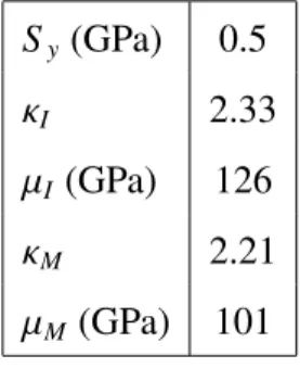
In what follows, all stresses are expressed in GPa and energies per unit of volume are given in J/mm3. Indeed, it was shown earlier that the total energy is proportional to eR2, so that the size of the inclusion does not impact the minimization in any way, it is thus simpler to present energies per unit of volume without specifying the inclusion size. The numerical values chosen to test our program were taken so as to match the properties of pure iron where a ferrite inclusion appears in an austenite matrix. Elastic constants were obtained from the calculations of the atomic model in Müller et al. (2007), and a typical value of the shear strength of steel was taken as the yield strength at the interface. Values are listed in table 1. In addition, let us
note that the numerical values resulting from calculations that are given below were obtained without linearization of matrix I for accuracy purposes, although the linearized algorithm gives energies that agree with the standard algorithm within 0.001% and is much faster.
Table 1: Numerical values of the parameters
Sy (GPa) 0.5
κI 2.33
µI (GPa) 126
κM 2.21
µM(GPa) 101
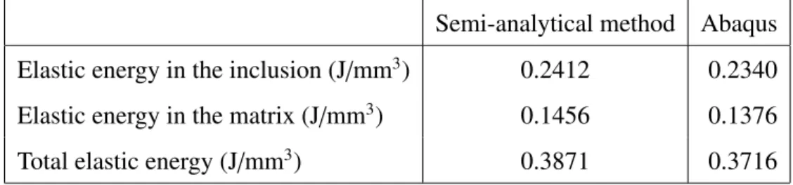
The method described previously was tested on a first loading case that purposely does not present the symmetries of the particular problem investigated here, so as to show the proper functioning of the Matlab program that was written. No eigenstrain was applied at this stage, and the loading case that was chosen was g : θ 7→ 0.1 sin+(θ), where sin+(θ) is the positive part of sin(θ). This means that for θ between 0 and π the sliding is equal to 0.1 sin(θ), and for θ between π and 2π it is equal to zero. It is readily seen that this loading case does not possess the symmetry with respect to either the Ox or the Oy axis. Furthermore, it is interesting because of the discontinuity of the derivative for θ = π and θ = 2π when considering g as a function of period 2π. This problem was solved with 30 Fourier coefficients in the expansion of the sliding. The displacements at the interface obtained with the solution presented in this contribution were then set on the nodes of a 2D Abaqus model using quadrangles of 0.1mm edges, and the elastic energies in the inclusion and in the matrix were computed. The total energy computed in Abaqus agrees with our results within 4%, as can be seen from table 2, and the Abaqus energies are slightly lower than the energies obtained with the present solution, which was to be expected for the matrix since it is of finite extent in the Abaqus model, but can only be attributed to both our approximation (a finite number of Fourier coefficients) and that of Abaqus (inherent to the finite elements method) for the inclusion.
The second loading case used to test the program was a case of eigenstrain with a zero yield strength at the interface. The components of the eigenstrain were also taken so as to be proportional to the eigenstrain experienced by austenite when changing into ferrite through
Table 2: Energies computed by our semi-analytical method and Abaqus
Semi-analytical method Abaqus
Elastic energy in the inclusion (J/mm3) 0.2412 0.2340
Elastic energy in the matrix (J/mm3) 0.1456 0.1376
Total elastic energy (J/mm3) 0.3871 0.3716
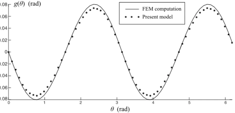
the Bain path (see Müller et al. (2007)), and were calculated from Müller et al. (2007). The proportionality factor is denoted by EBand is taken between 0 and 1, and the eigenstrain is thus given by: ε∗= E B 0.120 −0.210 (28)
This problem was solved for EB = 1 and taking advantage of the symmetries as mentioned in section 3, and using 10 functions of the type sin(2nθ) in the expansion of g(θ). Then the same eigenstrain was applied in a 2D Abaqus model similar to the one described before, with no friction between the inclusion and the matrix, and the sliding occurring in that simulation has been calculated for comparison. This calculation was made by linearly interpolating the initial positions of the points of the matrix coinciding with the nodes of the inclusion in the cur-rent configuration of the simulation. Given the size of the elements used, the fact that a linear interpolation was used, and the fact that in the Abaqus model the matrix is of finite extent, the results shown in figure 1 coincide nicely. Note that in the Abaqus model stress free boundary conditions were applied to the edge of the matrix instead of the zero displacement condition applied at infinity in the semi-analytical solution. These boundary conditions combined with the finiteness of the matrix makes it structurally more compliant, and a sliding of greater ampli-tude is thus expected, which is indeed the case. Zero displacement boundary conditions in the Abaqus model could have been used instead, but they would have made the matrix structurally stiffer, so that neither case is perfectly fitting. Since the Abaqus model is inherently imperfect due to discretization of the circles that slide against each other, the authors did not study any further the influence of the boundary conditions or the size of the domain considered.
Figure 1: Sliding calculated with our semi-analytical method and sliding calculated with Abaqus
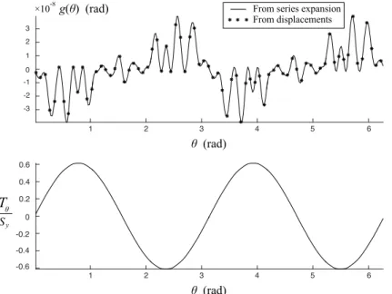
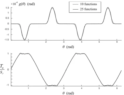
The program was then used to solve different problems with a non-zero yield strength in or-der to confirm the intuition on how it should perform depending on the eigenstrain applied and the yield strength at the interface. To do so, a yield strength of 0.5GPa is chosen, correspond-ing to the shear strength of a material like steel with a tensile strength of 1GPa and obeycorrespond-ing a Von Mises yield criterion, and EB varies between 0 and 1. For each case, the sliding obtained from the minimization is plotted along with the tangential component of the interfacial traction denoted by Tθ for comparison. Three main types of curves were obtained: for low enough eigenstrains (EB < 0.05), no sliding occurs (what is plotted is due to the finite precision of the calculation and is random noise) and|Tθ| is strictly below Sy (see figure 2); around EB = 0.05 sliding starts to occur locally, and where is does the criterion is saturated (i.e., |Tθ| = Sy) as shown in figure 3; finally for EB > 0.15 sliding occurs along the whole edge and the criterion is saturated everywhere on the edge as shown in figure 4. In addition, note that on figure 3 are shown the results for 10 and 25 functions in the expansion of g(θ), and it is clear that for 10 functions the presented method has already converged.
On figures 2 and 4, the solid line shows the sliding obtained directly from the Fourier coefficients obtained at the end of the minimization procedure, while the stars show the sliding deduced from the displacements of the inclusion and the matrix at the interface known from (12) and (17), where Pk and Dk are calculated from the Fourier coefficients of the sliding via (A.30) and (A.21) respectively. The sliding may indeed be deduced from the displacements by calculating the position x in the current configuration of a point XI(R, θ) = Rer(θ) of the inclusion via (12), and then by determining φ such that the point XM(R, φ) = Rer(φ) of the
matrix coincides with x in the current configuration via (17). Since this requires to calculate φ as a function of XM + uM, for which we do not have an analytical formula, this calculation was performed numerically by minimizing the function||x − XM(R, φ) − uM(R, φ)|| with respect to φ for several values of θ. The perfect agreement between the curve and the stars shows the consistency of the program when calculating the displacements from a prescribed sliding, since said sliding can be recovered from the displacements. Even though the program converges quickly with the number of functions in the expansion of g(θ), 20 functions were used to be as precise as possible and reduce fluctuations while keeping the running time relatively low. With 20 functions, the appearance of a Gibbs phenomenon due to the discontinuity of Tθ is clear on figure 4. Analysis of the Von Mises equivalent stress shows that for EB > 0.03, plasticity should occur in the medium, which means that the method presented here should only apply for relatively small eigenstrains, since it does not take plasticity into account. The maximum Von Mises equivalent stress indeed reaches 1GPa in the matrix for EB = 0.03.
Figure 2: Sliding and tangential component of the interfacial tractions obtained with Sy= 0.5GPa, EB= 0.03 and
Figure 3: Sliding and tangential component of the interfacial tractions obtained with Sy= 0.5GPa, EB= 0.05 and
respectively 10 and 25 functions in the expansion of g(θ)
Figure 4: Sliding and tangential component of the interfacial tractions obtained with Sy= 0.5GPa, EB= 0.15 and
20 functions in the expansion of g(θ)
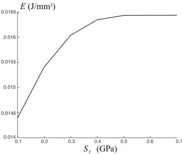
Finally, the confidence gained through these tests allowed us to study the evolution of the energy needed for the transformation to occur, see the introduction to section 2, as a function of Sy. For EB = 0.05, several values have been considered for Sy and the total energy needed for the transformation to occur is presented in figure 5. For Sy = 0, the inclusion can slide
perfectly against the matrix and Tθ = 0 at the interface. For Sy → +∞ we return to the case of perfect adherence, and imperfect adherence indeed reduces the total energy needed up to 12%.
Figure 5: Total energy calculated for EB= 0.05 and Syfrom 0 to 0.7GPa using 20 functions in the expansion of
g(θ)
5. Conclusion
In the present work, a semi-analytical solution to the problem of a sliding circular inclusion subjected to an eigenstrain and surrounded by an infinite matrix has been derived and applied to numerically evaluate the energy needed for a phase transition to occur. The sliding, due to localized plasticity (associated to a dissipation potential) has been evaluated within the frame-work of an energetic approach. The argument could be made that the elastic constants of steel at room temperature were used, when the austenite-ferrite phase transition occurs around 912◦C, at which point the elastic constants are greatly reduced. However, since the yield strength of the material also drops in a similar fashion, the conclusions remain valid. The relevance of taking into account the plastic dissipation at the interface was eventually showed: for an eigenstrain of only 5% the amplitude of that experienced during the phase change of austenite into ferrite, the energy difference between a free slip and a no slip interface condition amounts to 12% of the total mechanical energy needed for the transformation to occur without slip. For eigen-strains closer to the actual value, plastic dissipation at the interface and inside the inclusion and its surroundings can be assumed to have an even greater importance, however the framework developed here is unable to deal with strains as high as 20%.
This contribution is part of a more general framework that consists in modeling phase nu-cleation considering both the energy gain at the atomic scale when the crystal lattice is modified and elastic and dissipated energies at the scale of continuum mechanics. Thus a global energy can be minimized in order to determine phase nucleation allowing for discontinuities (i.e., that the product phase can appear with a certain size). Most attempts in this direction rely on Es-helby’s theory or perfectly sliding inclusions. Taking into account the plastic dissipation at the boundary of the inclusion, this contribution extends in 2D these previous inclusion methods while confirming the result that sliding does decrease the total energy needed for phase tran-sition to occur. However, the presented results show that for realistic eigenstrains involved in phase transition, plasticity should be be taken into account in the matrix and possibly in the inclusion. Furthermore an extension in 3D is also needed.
Appendix A. Coefficient determination
Substituting (10) and (14) in the second line of (22) one gets: N−1 ∑ k=−N+1 Dkei(k−1)θ= φ′(θ) N−1 ∑ k=−N+1 Pkei(k−1)φ(θ) (A.1)
Multiplying by 21πe−i(n−1)θfor n from 1− N to N − 1 and integrating from 0 to 2π yields:
Dn = N−1 ∑ k=−N+1 Pk 1 2π 2π ∫ 0 φ′(θ)ei((k−1)φ(θ)−(n−1)θ) dθ , −N + 1 ≤ n ≤ N − 1 (A.2)
Equation (A.2) can be written as an equation between matrices by introducing D and P the column matrices whose elements are Dn and Pk, and G the square matrix whose elements are
Gn,k = 21π
2π
∫
0
φ′(θ)ei((k−1)φ(θ)−(n−1)θ)dθ. The equation is then:
D= GP (A.3)
The displacement due to the eigenstrain is:
so that the left side of (22), denoted s(θ), may be written: s(θ) = (2 + ε∗xx+ ε∗yy− iκI+1 µI ℑ(ϕ1))Re −iθ+ 1 µI(κIϕ0− ψ0− D−1R) +(ε∗ xx− ε∗yy)Reiθ+ R N∑−1 k=−N+1 (ΛD)kei(k−1)θ (A.5)
where the column matrix D has been used again and where has been introduced the diagonal matrixΛ whose diagonal elements are:
Λn,n = − κI µI(n−1) , −N + 1 ≤ n ≤ −2 κI 2µI , n = −1 (κI−1) 2µI , n = 0 1 µI(n−1) , 2 ≤ n ≤ N − 1 (A.6)
Λ1,1 may be arbitrarily set since D1 = 0, so it will be set to zero. Multiplying by 21πe−i(n−1)θ
for n from−N+1 to N−1 and integrating from 0 to 2π yields 2N−1 equations that can be written as a matrix equation by introducing S the column matrix whose elements are21π
2π
∫
0
s(θ)e−i(n−1)θdθ:
S= −R A + R ΛD (A.7)
where A is a column matrix whose elements are:
An = 0, −N + 1 ≤ n ≤ −1 −(2 + ε∗ xx+ ε∗yy)+ iκ I+1 µI ℑ(ϕ1), n = 0 − 1 RµI(κIϕ0− ψ0− D−1R), n = 1 ε∗ yy− ε∗xx , n = 2 0, 3 ≤ n ≤ N − 1 (A.8)
The right side, denoted t(φ(θ)), can be written:
t(φ(θ)) = 2Re−iφ(θ)+ R
N−1 ∑ k=−N+1
whereΓ is the diagonal matrix whose diagonal elements are: Γn,n = 1 µM(n−1) , −N + 1 ≤ n ≤ −2 − 1 2µM , n = −1 − 1 µM , n = 0 − κM µM(n−1) , 2 ≤ n ≤ N − 1 (A.10)
Γ1,1 may also be set arbitrarily since P1 = 0, so it will be set to zero. Multiplying by 1
2πe−i(n−1)θ for n from−N + 1 to N − 1 and integrating from 0 to 2π yields once again 2N − 1
equations that can be written as a matrix equation by introducing T the column matrix whose elements are 21π 2π ∫ 0 t(φ(θ))e−i(n−1)θdθ: Tn= RBn+ R k=−N+1∑N−1 (ΓP)k 1 2π 2π ∫ 0 ei((k−1)ϕ(θ)−(n−1)θ)dθ (A.11)
where B, whose elements are Bn = 21π
2π
∫
0
2e−i(φ(θ)+(n−1)θ)dθ has been introduced. Introducing the square matrix I whose elements are In,k = 21π
2π
∫
0
ei((k−1)φ(θ)−(n−1)θ)dθ one can write:
T = R B + R I ΓP (A.12)
The first line of (22) may then be written, after simplifying by R:
ΛD = A + B + I ΓP (A.13)
Before going any further, let us recall briefly the dependencies of each term: • Λ depends on the elastic constants of the inclusion
• Γ depends on the elastic constants of the matrix
• A depends on the eigenstrain and the rigid body motion of the inclusion • B, G and I depend on the sliding
The problem that has to be solved is thus the following: D = GP ΛD = A + B + I ΓP (A.14)
without forgetting that D1 = 0, P1 = 0 and D0 ∈ R. System (A.14) is a linear system of
complex equations, but it cannot be inverted directly because of the fact that D0 ∈ R. Instead,
we need to separate between the real and imaginary parts of these equations to solve the system. To do so, let us write column matrices D and P as follows:
D = d + id′ P = p + ip′ (A.15)
where d, d′, p and p′ are real column matrices. We will write in an analogous fashion
A= a+ia′, B = b+ib′, G= g+ig′,Λ = l (Λ is already a real matrix) and I Γ = M = m+im′. Let us now write the first line of equation (A.14) for n= 0:
d0 =
N−1 ∑ k=−N+1
(g0,k + ig′0,k)(pk+ ip′k) (A.16)
and taking the imaginary part of this equation yields:
0= N−1 ∑ k=−N+1
(g0,kp′k + g′0,kpk) (A.17)
A value of k for which g0,k , 0 has to be selected, and it is assumed that this holds for k = 0 because in practice the sliding is going to be very small so that g0,0 = ℜ(G0,0) ≈ 1. Then, one
can write: p′0 = − 1 g0,0 ∑ k,0 (g0,kp′k + g′0,kpk)+ g′0,0p0 (A.18)
so that p′0 has been determined as a function of the pk and the other p′k. The first line of equation (A.14) can now be written, after separating the real part and the imaginary part:
dk = N∑−1 n=−N+1 (gk,npn− g′k,np′n), −N + 1 ≤ k ≤ 0 and 2 ≤ k ≤ N − 1 d′k = N∑−1 n=−N+1 (g′k,npn+ gk,np′n), −N + 1 ≤ k ≤ −1 and 2 ≤ k ≤ N − 1 (A.19)
Substituting (A.18) in this equation yields: dk = N∑−1 n=−N+1 (gk,n+ g′k,0 g0,0g ′ 0,n)pn+ ∑ n,0 (g ′ k,0 g0,0g0,n− g ′ k,n)p′n dk′ = N∑−1 n=−N+1 (g′k,n− ggk,0 0,0g ′ 0,n)pn+ ∑ n,0 (gk,n− gk,0 g0,0g0,n)p ′ n (A.20)
Thus the column matrix obtained by concatenating dk for k , 1 and d′k for k , 0, 1 is expressed as a certain matrix multiplied by the analogous concatenation for pkand p′k. It is not necessary to take into account the equations obtained for k = 0 because they yield 0=0. The concatenations just mentioned will be denoted ˜d and ˜p, and the matrix linking the two ˜g so that
one has:
˜
d= ˜g ˜p (A.21)
Writing in the same fashion the second line of equation (A.14) yields: lk,kdk = ak+ bk+ N∑−1 n=−N+1 [ mk,npn− m′k,np′n ] lk,kdk′ = a′k+ b′k+ N∑−1 n=−N+1 [ m′k,npn+ mk,np′n ] (A.22)
For k = 1 one has: 0 = a1+ b1+ N∑−1 n=−N+1 [ m1,npn− m′1,np′n ] 0 = a′1+ b′1+ N∑−1 n=−N+1 [ m′1,npn+ m1,np′n ] (A.23)
but from (A.8) one has a1 = −R1µIℜ(κIϕ0− ψ0)+ µ1Id−1and a′1 = − 1
RµIℑ(κIϕ0− ψ0)−
1 µId−1
1 RµIℜ(κIϕ0− ψ0) = 1 µId−1+ b1+ N∑−1 n=−N+1 [ m1,npn− m′1,np′n ] 1 RµIℑ(κIϕ0− ψ0) = − 1 µId−1+ b ′ 1+ N∑−1 n=−N+1 [ m′1,npn+ m1,np′n ] (A.24)
so thatℜ(κIϕ0− ψ0) andℑ(κIϕ0− ψ0) can be calculated as functions of pk for k, 1 and p′k for k , 0, 1 since d−1and p′0are known as functions of them.
For k = 0 and considering only the imaginary part one has:
0= a′0+ b′0+ N−1 ∑ n=−N+1 [ m′0,npn+ m0,np′n ] (A.25)
but from (A.8) one has a′0 = κI+1
µI ℑ(ϕ1) so: κI + 1 µI ℑ(ϕ1)= −b′0− N−1 ∑ n=−N+1 [ m′0,npn+ m0,np′n ] (A.26)
so thatℑ(ϕ1) can be calculated as a function of pk for k, 1 and p′kfor k , 0, 1 for the same reason as previously.
Finally, let us substitute (A.18) in (A.22): lk,kdk = ak+ bk+ N∑−1 n=−N+1 (mk,n+ m′k,0 g0,0g ′ 0,n)pn+ ∑ n,0 (m′k,0 g0,0g0,n− m ′ k,n)p′n lk,kdk′ = a′k+ b′k+ N∑−1 n=−N+1 (m′k,n− mk,0 g0,0g ′ 0,n)pn+ ∑ n,0 (mk,n− mk,0 g0,0g0,n)p ′ n (A.27)
Taking the first line for k, 1 and the second line for k , 0, 1, one can write these equations as was previously done introducing the analogous concatenations ˜d, ˜a, ˜b and ˜p and the matrices
˜l and ˜m:
˜l ˜d= ˜a + ˜b + ˜m ˜p (A.28)
The quantities κIϕ0− ψ0 and ℑ(ϕ1) are not part of the system any more, and substituting
(A.21) yields:
and inverting the matrix yields:
˜p= (˜l ˜g − ˜m)−1( ˜a+ ˜b) (A.30)
The problem is now completely solved: all the pk for k , 0 and the p′k for k , 0, 1 are determined, but p′0 is known from (A.18). One can then deduce the dk for k , 0 and the d′k for k , 0, 1 from (A.20), and then κIϕ0− ψ0 andℑ(ϕ1) from (A.24). From this we get P and
D, so that one can compute the coefficients ϕk andψk from (11), and the coefficients αk andβk from (15). The holomorphic potentials are then obtained everywhere in the inclusion and in the matrix, and finally the displacement field and the stress field are obtained in the inclusion and in the matrix.
Ammar, K., Appolaire, B., Cailletaud, G., Forest, S., 2009. Combining phase field approach and homogenization methods for modelling phase transformation in elastoplastic media. Eu-ropean Journal of Computational Mechanics/Revue Européenne de Mécanique Numérique 18, 485–523.
Bain, E.C., Dunkirk, N., 1924. The nature of martensite. trans. AIME 70, 25–47.
Delannay, L., Jacques, P., Pardoen, T., 2008. Modelling of the plastic flow of trip-aided mul-tiphase steel based on an incremental mean-field approach. International Journal of Solids and Structures 45, 1825–1843.
Eshelby, J.D., 1957. The determination of the elastic field of an ellipsoidal inclusion, and related problems, in: Proceedings of the Royal Society of London A: Mathematical, Physical and Engineering Sciences, The Royal Society. pp. 376–396.
Fedelich, B., Ehrlacher, A., 1997. An analysis of stability of equilibrium and of quasi-static transformations on the basis of the dissipation function. European journal of mechanics. A. Solids 16, 833–855.
Fischer, F., Reisner, G., 1998. A criterion for the martensitic transformation of a microregion in an elastic–plastic material. Acta materialia 46, 2095–2102.
Hensl, T., Mühlich, U., Budnitzki, M., Kuna, M., 2015. An eigenstrain approach to predict phase transformation and self-accommodation in partially stabilized zirconia. Acta Materi-alia 86, 361–373.
Huang, J.H., Furuhashi, R., Mura, T., 1993. Frictional sliding inclusions. Journal of the Me-chanics and Physics of Solids 41, 247–265.
Jasiuk, I., Tsuchida, E., Mura, T., 1987. The sliding inclusion under shear. International journal of solids and structures 23, 1373–1385.
Kurdjumow, G., Sachs, G., 1930. Über den mechanismus der stahlhärtung. Zeitschrift für Physik 64, 325–343.
Lambert-Perlade, A., Gourgues, A.F., Pineau, A., 2004. Austenite to bainite phase transfor-mation in the heat-affected zone of a high strength low alloy steel. Acta Materialia 52, 2337–2348.
Mielke, A., 2003. Energetic formulation of multiplicative elasto-plasticity using dissipation distances. Continuum Mechanics and Thermodynamics 15, 351–382.
Müller, M., Erhart, P., Albe, K., 2007. Analytic bond-order potential for bcc and fcc iron—comparison with established embedded-atom method potentials. Journal of Physics: Condensed Matter 19, 326220.
Mogilevskaya, S., Crouch, S., 2002. A galerkin boundary integral method for multiple circular elastic inclusions with homogeneously imperfect interfaces. International Journal of Solids and Structures 39, 4723–4746.
Mura, T., Jasiuk, I., Tsuchida, B., 1985. The stress field of a sliding inclusion. International Journal of Solids and Structures 21, 1165 – 1179.
Mura, T., Mori, T., Kato, M., 1976. The elastic field caused by a general ellipsoidal inclusion and the application to martensite formation †. Journal of the Mechanics and Physics of Solids 24, 305 – 318.
Muskhelishvili, N., 1953. Some Basic Problems of the Mathematical Theory of Elasticity. Noordhoff International Publishing, Groningen. 2nd edition (1977).
Nishiyama, Z., 1934. X-ray investigation of the mechanism of the transformation from face centered cubic lattice to body centered cubic. Sci. Rep. Tohoku Univ 23, 637–664.
Ru, C., 1998. A circular inclusion with circumferentially inhomogeneous sliding interface in plane elastostatics. Journal of applied mechanics 65, 30–38.
Saotome, Y., Iguchi, N., 1987. In-situ microstructural observations and micro-grid analyses of transformation superplasticity in pure iron. Transactions of the Iron and Steel Institute of Japan 27, 696–704.
Tsuchida, E., Mura, T., Dundurs, J., 1986. The elastic field of an elliptic inclusion with a slipping interface. Journal of applied mechanics 53, 103–107.
Zhong, Z., Meguid, S., 1997. On the elastic field of a shpherical inhomogeneity with an imper-fectly bonded interface. Journal of elasticity 46, 91–113.