Heat and Mass Budgets of the Warm Upper Layer of the Tropical Atlantic Ocean in
1979–99
F. VAUCLAIR*ANDY.DUPENHOAT
Laboratoire d’Etudes en Ge´ophysique et Oce´anographie Spatiales, Toulouse, France G. REVERDIN
Laboratoire d’Oce´anographie Dynamique et Climatologie, Paris, France (Manuscript received 26 November 2002, in final form 27 August 2003)
ABSTRACT
The mass and heat budgets of the warm upper-ocean layer are investigated in the equatorial Atlantic using in situ observations during the period 1979–99, which encompassed a series of warm events in the equatorial Atlantic. The warm water layer is defined as the layer having an in situ temperature higher than 208C, which is within the core of the equatorial thermocline. The geostrophic transport is calculated by combining gridded temperatures with historical salinity data. The Ekman transport is estimated from observed wind data or model-based wind products. The change in warm water volume is then compared with the horizontal mass convergence, and the residuals are determined. The heat budget of the upper layer is investigated in the same way. Three regions are considered: the equatorial band between 88N and 88S to study the meridional redistribution of the warm water and two boxes (western and eastern boxes) to investigate the zonal redistribution of the warm water. Mass and heat budget variability in the equatorial band is discussed in relation to the zonal wind variability. The authors discovered that during the development of an equatorial warm event the meridional net divergence first decreases, reaching its minimum as the warm event matures. Meridional divergence increases again as conditions become normal in the equatorial band. The vertical velocity through the 208C isotherm also reveals variations consistent with this scenario. Cross-isotherm mass transport decreases during warm events. The heat budget residual is more difficult to interpret. The average value is consistent with heat loss through turbulent mixing at the base (208 isotherm), but the fluctuations are most likely noise, resulting mainly from the limited accuracy of the model surface heat fluxes used.
1. Introduction
The tropical Atlantic Ocean varies greatly, according to the seasons, in surface temperature (Merle 1980a), currents (Arnault 1987), and in its equatorial heat bud-get and upwelling (Merle 1980b; Gouriou and Rev-erdin 1992). In addition, its interannual variability sug-gests different modes of sea surface temperature (SST) variability related to atmospheric variability. The first is the Atlantic counterpart of the Pacific El Nin˜o– Southern Oscillation (ENSO) with a relaxation of the equatorial trade winds inducing a redistribution of warm water in the equatorial band and a decrease in the thermocline slope and zonal heat content gradient (Merle 1980b), which could be the result of a damped
* Current affiliation: Department of Physical Oceanography, Uni-versity of Sa˜o Paulo, Sa˜o Paulo, Brazil.
Corresponding author address: Yves du Penhoat, LEGOS, 14 Ave. Edouard Belin, 31400 Toulouse, France.
E-mail: [email protected]
oscillatory mode of the coupled Atlantic Ocean–at-mosphere (Zebiak 1993). The mature phase is char-acterized by a warming of the eastern equatorial basin, a modification of the African monsoon, and a south-ward and eastsouth-ward displacement of the convection zone. The second variability mode was originally iden-tified through the decadal fluctuations of rainfall over the Brazilian Nordeste region, which is associated with a dipolelike meridional gradient of SST anomalies (Servain 1991; Nobre and Shukla 1996). The spectral characteristics of the SST variability in different re-gions of the Atlantic and the relative coupling between these different regions is still a subject of discussion (e.g., Enfield and Mayer 1997; Carton et al. 1996). Servain et al. (1999) suggest that the variability in the northern center of action of the dipole and the eastern equatorial Atlantic are linked by the meridional posi-tion of the intertropical convergence zone (ITCZ) and its anomalies.
The tropical Atlantic variability has been linked to other climate systems such as ENSO and the North At-lantic Oscillation (NAO) on the basis of surface
obser-Until now, most studies of the variability have used surface observations or model simulations. They sug-gest that ocean dynamics play an important role in the coupling between SST variability in different regions and, in particular, in significant variations in the strength of the equatorial upwelling on seasonal to interannual time scales associated with the interannual variability modes. However, no study based on observations has attempted to quantify the exchange of warm water be-tween the equatorial region and higher latitudes and across the thermocline on interannual time scales.
The purpose of this paper is to investigate the upper-ocean mass and heat balance and to address the question of warm water volume variability during warm events in the tropical Atlantic Ocean, in particular what per-centage of its variability is related to horizontal redis-tribution and what percentage is related to transfers through the lower boundary (variability of upwelling). Geostrophic transports have been estimated from ocean density analyses and Ekman transport using either wind products based on observations [Florida State Univer-sity (FSU) products] or on atmospheric model reanalysis [National Centers for Environmental Prediction–Na-tional Center for Atmospheric Research (NCEP– NCAR)]. Meinen and McPhaden (2000, 2001) used a similar method to address a number of issues surround-ing the warm water budget of the tropical Pacific Ocean during 1993–99. In particular, they confirmed that there are significant movements of warm water in and out of the equatorial region (bound at 88N and 88S in their study) and they paid special attention to the 1997–98 ENSO event. Gouriou and Reverdin (1992) investigated the seasonal isopycnal and diapycnal circulation of the upper equatorial Atlantic during a series of cruises in 1983–84. They found a seasonally varying meridional convergence at the undercurrent level but a larger me-ridional divergence in the surface layer in the central part of the basin. In section 2, we describe the data and method used. In section 3 we describe the geostrophic and Ekman fluxes and the associated mass and heat transports. In section 4 we describe heat and mass bud-get variability. Section 5 contains a discussion of our results, a summary, and conclusions.
to estimate Ekman transports. The FSU wind dataset combines measurements from ships and buoys to pro-vide monthly wind pseudostress on a 28 by 28 grid (Stri-cherz et al. 1997; Servain et al. 1987). FSU wind pseu-dostress values were converted into wind stress using a constant drag coefficient of 1.2 3 1023 (Sirven et al.
1998) and an air density of 1.2 kg m23. The second wind dataset was obtained from the NCEP–NCAR re-analysis and derived from an atmospheric general cir-culation model, which assimilates measurements from many data sources. The entire data assimilation system has been described by Kalnay et al. (1996). The dif-ferences between wind products used in this study imply uncertainty in the calculation of the Ekman transport, which is strongly wind dependent.
A comparison of the two products reveals differences, both for the mean and the variability. The FSU easterlies are stronger in the equatorial band (58N–58S) (Fig. 1). The mean ITCZ is located farther north in the FSU product than in NCEP–NCAR. The rms difference be-tween FSU and NCEP–NCAR zonal winds is larger in the subtropics and in the western part of the equatorial band (Fig. 2). In the Gulf of Guinea and in the eastern part of the equatorial band, the variability is quite similar for both products. For the meridional winds, a maximum rms difference is found in upwelling regions where the SST variability is strongest. Correlation between the two products is more than 0.9 in the ITCZ region, between 0.7 and 0.9 in the northern subtropical gyre, and between 0.5 and 0.8 in the southern subtropical gyre (figure not shown). The lower correlation in the southern tropical Atlantic is due to the lack of in situ data in that region. At the equator, the two products indicate a strengthening of the easterlies between 1964 and 1981–82. Then, NCEP–NCAR easterlies decreased whereas the FSU easterlies remained strong but with an increasing inter-annual variability. Trends toward increasing winds in the FSU product might be an artifact due to changes in measurement techniques (Posmentier et al. 1989; Car-done et al. 1990). Despite these differences, the two products show coherent patterns of variability and mean circulation. In particular, the larger climatic events are well identified in both products.
FIG. 1. Average differences between FSU and NCEP–NCAR (a) zonal and (b) meridional winds (N m22).
The dynamic height was calculated in order to deter-mine geostrophic velocities relative to a depth of 500 m from the TAOSTA gridded dataset. Since the TAOSTA dataset does not provide salinity, we used historical data (Levitus and Boyer 1994) to derive a mean temperature– salinity (T–S) relation at each grid point. From this T–S and the temperature data, we constructed a pseudosalinity profile associated with each temperature profile. We fur-ther neglected currents at 500 m in depth, which cannot be estimated from our data.
From 38N and 38S toward the North and South Poles respectively, zonal geostrophic velocities were calcu-lated using the centered first-order derivative of the dy-namic height based on the geostrophic formulation. Be-tween 38N and 38S, we approximated the zonal velocity by the second derivative of the dynamic height using a second-order finite difference following Bryden and Brady (1985) and Picaut et al. (1989):
2
] D [D(38N) 1 D(38S) 2 2D(08)]
5 , (1)
2 2 2
] y Dy
with D being the dynamic height.
The horizontal transports were estimated by combin-ing the geostrophic and Ekman components. Ekman transports were calculated from both NCEP–NCAR and FSU wind stress products using the standard technique described in Pond and Pickard (1983). Because of the TAOSTA grid (28 mesh in latitude and longitude), the first grid point out from the equator to calculate the Ekman transport is at 38N and 38S. These boundaries are coherent with the previous study of Meinen and McPhaden (2000). Within 38N–38S, our assumption im-plicitly took this contribution to the zonal transport into account. Based on earlier work in the Pacific, we expect that this corresponds fairly well to the transport of the zonal current (Meinen and McPhaden 2000; Picaut et al. 1989).
FIG. 2. Rms differences between FSU and NCEP–NCAR monthly wind stresses (N m22): (a)
zonal and (b) meridional winds.
This study focuses on the warm water layer (between the surface and the depth of the 208C isotherm) in three regions: the equatorial band bounded by 88N–88S, the western box bounded by 88N–58S and 388–208W, and the eastern box bounded by 58N–88S and 208W–28E (Fig. 3). Heat and mass budgets (limited in depth by the 208C isotherm) were computed in each region. For the equatorial band, the northern boundary was chosen as 88N, roughly the latitude of a change of sign in the seasonal variability in thermocline depth. The southern boundary was chosen as 88S in order to minimize errors induced by the lack of data that become too large in the southern central part of the tropical Atlantic (Vau-clair and du Penhoat 2001). Taking this boundary closer to the equator would have resulted in greater uncertainty in the meridional currents and in the heat budgets, un-resolved contributions by eddies to meridional heat transport becoming more important. This latitude band 88N–88S also captured most of the current variability linked with the equatorial dynamic and has been
re-tained in various studies of the equatorial mass balance (Roemmich 1983). The two other regions used in this study (eastern and western equatorial boxes on either sides of the 208W meridian) were chosen to separate areas of maximum variability identified in the statistical study of Vauclair and du Penhoat (2001). They also correspond to areas with good data coverage and avoid issues of transports by boundary currents and their re-circulations that are poorly resolved in the TAOSTA analysis and might result in errors in the budgets of the equatorial box. The 208C isotherm was chosen as the base of the warm water layer because it is a good rep-resentation of the thermocline depth in the tropical At-lantic and rarely surfaces within 88 of the equator.
The choice of the 208C isotherm (S20) as the lower bound of the warm water was also adopted by Meinen and McPhaden (2000) for the equatorial Pacific, who found large fluxes across this boundary. We refer to the warm water volume (WWV) as the volume of this layer in the region investigated, written as
FIG. 3. TAOSTA mean 208C isotherm depth and schematic boxes used in this study: WB is the western box, and EB is the eastern box.
x2 y2
WWV5
E E
D20dx dy. (2)x1 y1
Because seawater is nearly incompressible, the rate of change of WWV is balanced by volume transports across box boundaries, that is by the horizontal net (geo-strophic plus Ekman) transports, by surface transport [precipitation minus evaporation (P2 E)], and by the cross-S20 transport. The P2 E transport is negligible when compared with the other contributions, which is similar to what was found in the equatorial Pacific (Mei-nen and McPhaden 2000). Neglecting its variability only adds a little uncertainty [order of 0.05 Sv (Sv [ 106
m3s21)] to the estimates of the cross-S20 transport. The
cross-S20 transport is estimated as the difference be-tween the rate of change of WWV and the net transport across the vertical boundaries of the box:
d(WWV) 5
EE
U dSh 1EE
w dS .20 (3)dt S S20
The expression on the left-hand side is the variation rate of the warm water volume and the first term of the expression on the right-hand side is the horizontal trans-port across the vertical boundaries of the box, while the second term is the transport across the 208C isotherm (lower boundary of the box).
The cross-S20 transport is an important climatic var-iable as a positive transport (entrainment) is expected to be associated with cool, nutrient-rich surface waters. Because this upwelled water had to warm during this vertical transport, it is associated with a subsurface dia-batic convergence of heat fluxes (diapycnal heating
terms). Most of these are associated with downward turbulent heat fluxes and are thus associated with a heat loss for the surface layer. Therefore, this will also have an effect on the heat budget of the WWV, which is a strong reason for considering the heat budget of the upper layer at the same time as the mass budget. Heat transport was calculated with the temperature referenced to 208C (Niiler and Stevenson 1982). With this refer-ence, the budget is primarily a balance between net sur-face heat fluxes (from NCEP–NCAR), horizontal trans-port (relative to 208C), and vertical turbulent heat trans-ports (appendix A). Thus this provides an estimate of the vertical turbulent heat flux independently of the cross-S20 transport, which can be used to check the consistency of these budget estimates.
In order to focus on interannual variability, seasonal variations have been removed by applying a 12-month running mean on all time series. It would be interesting to investigate seasonal deviations from the seasonal cy-cle, but uncertainties in the budgets derived from the observed fields are too great to permit this. The four events (1983–84, 1987–88, 1992–93, and 1997–98) identified in the statistical study of Vauclair and du Pen-hoat (2001) were chosen for a closer examination of the heat and mass budget variability.
3. Transports and variability in warm water volumes
The average S20 shoals in the eastern equatorial At-lantic similarly to what is observed in the eastern Pa-cific. Changes observed in the S20 structure on
inter-FIG. 4. (a) Mean zonal component (1979–99) of the geostrophic velocity (cm s21) and (b) the
associated rms variability.
annual time scales correspond to changes in the warm water volume and induce displacements of warm water through the associated geostrophic currents that hori-zontally redistribute mass and heat in the equatorial At-lantic. Here, we will focus on the currents and horizontal transports. The annual mean zonal geostrophic veloci-ties computed over the 20 years analyzed reproduces the well-known characteristics of the zonal near-surface current (Fig. 4), with its succession of eastward and westward currents. North of 108N, the North Equatorial Current (NEC) flows westward at a mean speed between 5 and 10 cm s21and with an rms variability of less than
6–7 cm s21. Between 108 and 38N, the North Equatorial
Countercurrent (NECC) flows eastward against the trade winds at a speed between 5 and 20 cm s21and with an
rms variability between 8 and 16 cm s21. This
coun-tercurrent is well established between June and Decem-ber but is harder to distinguish between January and June. Closer to the equator, one finds the strongest cur-rent, the South Equatorial Current (SEC) flowing
west-ward with a speed reaching 30 cm s21. This current is
divided into two branches on both sides of the equator with maxima located at 28N and 48S, as was found in previous studies by Arnault (1987) and Richardson and McKee (1984). The rms variability of the zonal com-ponent of the geostrophic velocity reaches a maximum near 28–38N, which corresponds to the region of strong meridional shear between the northern branch of the SEC and the NECC.
In order to characterize the main pattern of interan-nual variability for geostrophic velocity, EOFs were computed for each velocity component. Only results for the zonal geostrophic velocity are shown in Fig. 5. The first mode is associated with the SEC interannual var-iability. The associated temporal function shows a rapid succession of strong (positive) and weak (negative) SEC. There is some coherency with the east–west con-trast in depth of the 208C isotherm (S20) along the equa-tor illustrated by the third principal component of the analysis of S20 in Vauclair and du Penhoat (2001, their
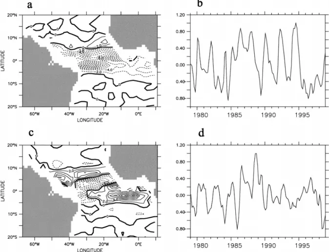
FIG. 5. First two EOFs (18% and 9% of the total variance, respectively) of the zonal component of the geostrophic velocity anomalies, referred to 500 dbar. (a), (c) The spatial structures and (b), (d) the associated time series for the (top) first and (bottom) second modes.
Fig. 12). Increased equatorial slope of S20 (shallow in east and deep in west) tends to follow periods with a strong SEC. This seems to be the case in 1983, 1990, and 1992. In 1984, a weak SEC also precedes a reduced equatorial slope. However, at other times this does not hold. For example, in 1987, the large SEC at the end of the year is not associated with an identified feature in the S20 equatorial slope. The second mode of the zonal current (Fig. 5c) characterizes the NECC vari-ability with an opposite sign in the northern branch of the SEC. Another pattern of strong variability can be seen in the Gulf of Guinea in the southern branch of the SEC.
Figure 6 illustrates the geostrophic transport (above the 208C isotherm) calculated across 208W between 58N and 58S and the SST anomalies in the eastern box, and it looks like the mechanism described in Carton and Huang (1994). The zonal transports are westward most of the time except, for example, in 1984 and 1987 during the warm event (the expected error is about 1 Sv for the interannual signal and 5 Sv for the total signal; see appendix B). The good correlation between 1980 and
1985 indicates that, for this particular event, the zonal geostrophic transport variability at 208W was associated with SST anomalies in the east. The zonal wind in the western box decreased significantly in the second half of 1983 and the beginning of 1984 and was associated with a decrease of the westward geostrophic current at 208W (which reversed during the mature phase of the warm event in 1984). For the 1987–88 warm event this relation did not hold, confirming the results of Vauclair and du Penhoat (2001): the 1987–88 events involved other mechanisms than just the equatorial mode.
Geostrophic transports are toward the equator across the 88N and 88S sections (Fig. 7) and reveal a significant interannual variability. For example, during 1983, the meridional transport strengthened, resulting in a large geostrophic convergence at the end of 1983. As the 1984 warm event developed, the geostrophic convergence weakened.
The NCEP–NCAR and FSU wind products are used to calculate Ekman transport across 88N and 88S and across the boundaries of the boxes defined in section 2 (Fig. 8). The whole Ekman transport is assumed to take
FIG. 6. (a) Geostrophic transport (Sv) calculated across 208W in-tegrated above the 208C isotherm and between 58N and 58S (solid) and SST anomalies in the eastern box (dashed). (b) Zonal wind (N m22) average in the western box. A 12-month running mean filtering
was applied.
FIG. 7. Geostrophic transport (Sv) calculated across 88N (solid), 88S (dashed), and the divergence (dotted). A 12-month running mean filtering was applied.
FIG. 8. Ekman transports (Sv) calculated across (a) 88N and (b) 88S, from FSU winds (solid) and from NCEP–NCAR winds (dashed). A 12-month running mean was applied. place above the 208C isotherm; that is, the depth of the
Ekman layer is shallower than the depth of the 208C isotherm, which might not always be true (Chereskin and Roemmich 1991). Because the Coriolis parameter
vanishes at the equator, meridional Ekman transport is calculated poleward of 28S and 28N and is assumed to vary linearly between the two latitudes.
The mean meridional Ekman transport across 88N is 9.25 Sv for FSU and 11.97 Sv for NCEP–NCAR. At 88S the mean Ekman transport is 210.25 Sv for FSU and 210.94 Sv for NCEP–NCAR. The two estimates agree well after 1982 south of the equator, but there are no similarities between the two time series north of the equator. The meridional Ekman transport is much larger than the zonal Ekman transport. The interannual vari-ability of the meridional Ekman transport is of the same order as the one for the geostrophic transport. During the warm event in 1984 the trade wind relaxation in-duced a particularly large diminution of the Ekman di-vergence. During the 1987–98 event, Ekman divergence was also abnormally low in 1997 whereas it increased in 1998.
FIG. 9. (a) Net mass transports (geostrophic1 Ekman; Sv) across 88N (solid) and 88S (dashed). Positive transport is northward. (b) Net mass divergence between 88N and 88S and WWV calculated between 88N and 88S (dashed line; 1013m3). A 12-month running mean was
applied.
In what follows we present only results computed with FSU winds. At 88N and 88S the net transport com-puted above the 208C isotherm is always poleward (Fig. 9a). It is 7 Sv (62 Sv) at 88N and 28 Sv (62 Sv) at 88S; thus the meridional net divergence equals 15 Sv (64 Sv). This equatorial divergence has an interannual variability closely related to the events identified in Vau-clair and du Penhoat (2001). For example, in 1982, the meridional divergence was abnormally strong simulta-neous with the negative SST anomalies, weak heat con-tent, and a shallow thermocline in the equatorial band. This corresponded to a weak geostrophic convergence and strong easterlies. During the development of the warm phase in 1983, the meridional net divergence weakened and reached its minimum as the warm phase matured at the end of 1983 and early 1984.
Associated with these transports are large variations of the WWV anomalies (Fig. 9b), in particular during the 1983–84 event (the 12-month running mean reduces them). During that event there was an accumulation of warm water from June 1983 until the beginning of 1984, then a diminution that ended at the end of 1985. In 1993 and 1997, there was also an accumulation of warm water that created favorable conditions for the development of the warm phase toward the end of 1993 and the beginning of 1998. For 1984, 1993, and 1998 the same
scenario occurred, namely, a few years of relative sta-bility of the WWV preceding a sharp increase of the WWV followed by a decrease. For the 1987–88 event, the scenario is different and we have not observed a period of weak WWV variability preceding the accu-mulation of warm water in the equatorial band [in agree-ment with Vauclair and du Penhoat (2001)].
As found by Meinen and McPhaden (2001) for the equatorial Pacific, this study shows that WWV vari-ability in the equatorial Atlantic is closely linked to variability of the net equatorial divergence. In the Pa-cific, Meinen and McPhaden (2001) showed that the accumulation of warm water, associated with a dimi-nution of the net divergence, resulted primarily from a decrease of the southward net transport across 88S com-bined with an anomalous increase of the eastward flow across 1568E. In the present study, with a longer time series (20 yr), we were able to study different events. For the 1983–84 and 1997–98 events, the diminution of the net divergence involved a diminution of the north-ward transport across 88S and of the southward transport across 88N. Instead, in 1987–88 the diminution of the net divergence was primarily due to the variation of the transport across 88N. In 1983–84 and 1997–98, warm events were combined with an anomalous increase of the eastward flow across 208W (Fig. 6), showing sim-ilarities with the study of Meinen and McPhaden (2001). Thus, concerning the WWV and the net divergence var-iabilities, the equatorial Atlantic dynamics seem to be more complicated than in the equatorial Pacific.
When considering the mass budget [Eq. (3)], we find that the contribution of the net horizontal mass trans-port is always larger than the rate of change of the WWV. Therefore, there is a variable mass deficit that has to be balanced by a vertical flow across the 208C isotherm (upwelling). This vertical transport can be converted into a vertical upwelling velocity across the 208C isotherm assuming arbitrarily that most of the upwelling transport occurs between 28N and 28S. The mean vertical velocity estimated by this method is 85 cm day21 with an uncertainty of 3 cm day21 and an
rms variability of 31 cm day21 (see appendix B) for
the equatorial band. We should point out that our anal-ysis poorly resolves the western boundary transports in the surface layer. In particular, we expect a poleward transport at 88N along South America that would con-tribute to a larger average upwelling. However, we do not know how variability in the poorly resolved west-ern boundary currents will contribute to the variability in vertical velocities. Figure 10 shows significant in-terannual variability of the vertical velocity related to the zonal wind variability in the equatorial band (co-efficient of correlation of20.4 at a significance level of 99%). A minimum of the vertical velocity often lagged by a few months the beginning of the relaxation in the winds. This is observed in 1983, at the end of 1987, at the beginning of 1992, and in 1997. In 1982, the upwelling reached a maximum (956 3 cm day21
FIG. 10. Zonal winds average between 88N and 88S (solid line; N m22) and vertical velocity (dashed line; cm day21) in the equatorial
band. A 12-month running mean was applied.
FIG. 11. (a) Warm water volume and (b) interannual anomalies calculated in the western box (solid line) and in the eastern box (dashed line). Units are in meters cubed. on average for the whole width of the basin) and
weak-ened significantly at the end of 1983 and the beginning of 1984. A second important maximum was observed for 1994 when the vertical velocity reaches 976 3 cm day21.
Surface geostrophic currents and zonal transport across meridional sections show that the zonal warm water displacement is also significant, suggesting that there might be large differences between the eastern and western parts of the equatorial domain. We there-fore performed the same calculation for the eastern and the western boxes defined in section 2. WWV mean values are 7.423 1014m3for the equatorial band (88N–
88S), 2.62 3 1014 m3 for the western box, and 2.23
1014 m3 for the eastern box. WWV variations in the
eastern box and in the western box are highly corre-lated (c5 0.76 with a level of significance of 99%) for a 3-month lag (western box leading the eastern box) (Fig. 11). Deviations from the average seasonal cycle
interannual variability of the vertical transports (or ver-tical velocities) across S20 in the eastern and western boxes are also correlated with a maximum 12-month lag (western box leading the eastern box; c5 0.55 at a significance level of 99%). We have no explanation for this longer lag as compared to the one in WWV. There is thus a large interannual variability of the equa-torial upwelling across S20. The time series suggest that the upwelling is strong during cold equatorial ep-isodes, but weakens as a warm phase of an equatorial event developed (e.g., in 1982–84 and 1996–98).
4. Heat budget
The heat budget was calculated for the equatorial band (88N–88S) and for the two boxes defined in sec-tion 2. In this paper we present results for only the equatorial band. The transport calculation was refer-enced to 208C so that estimation of vertical advection across the 208C isotherm does not contribute to the budget (see appendix A). The surface heat fluxes are from the NCEP–NCAR reanalysis. Thus, the residual of the heat budget equation corresponds to the vertical transport due to turbulent diffusion across S20 (in
ad-dition to a small downward shortwave flux term) (Ni-iler and Stevenson 1982). The heat budget equation
can be written in a final form as follows (see appendix A for details and notations):
](^T& 1 T0)
rCp
EE
w0T0 ds 5 2EE
Foa dS2 rCpEE
^U &(T 2 20) dS 2h rCpEEE
dV1 R, (4) ]tS30 S0 S V
(I) (II) (III) (IV)
FIG. 12. Four components of the heat budget (pW) in the eastern box: Ekman divergence (solid line), geostrophic convergence (dashed line), ocean–atmosphere heat transfer (dotted), and rate of change of heat storage (dashed–dotted). A 12-month running mean was applied.
with V the considered fluid volume, S20 the 208C
iso-therm surface representing the lower boundary of the box, S the vertical surface bounding the box, S0 the
ocean surface in contact with the atmosphere, and w0 the vertical velocity fluctuation across the 208 isotherm. The left-hand side of Eq. (4) (term I) represents the heat transport across S20 (208C isotherm surface) due to the turbulent diffusion and is estimated from the terms on the right-hand side. The first term of the right-hand side (II) is the net heat flux across the ocean surface (with contributions from the net shortwave flux, solar flux, and sensible and latent heat flux). This is given from the NCEP–NCAR reanalysis with uncertainties discussed at the end of appendix B. The second term (III) represents the horizontal heat transport referenced to 208C, and the third term (IV) represents the heat storage associated with the temperature changes. Here R corresponds to hori-zontal transport at scales that are not resolved in the analysis; it has not been considered in this study.
a. Meridional heat transport
Heat and mass flux variations are highly correlated across both 88N and 88S. This is not unexpected and has already been noted by Philander (1986). If we note
V the velocity normal to the surface and T the
tem-perature referred to 208C, the heat flux is VT 5VT 1 V9 1 T9 1 V9T9, where the prime refers to theT V
fluctuations from the mean state. The temperature fluc-tuations T9 are much lower than the mean temperature, whereas velocity fluctuations V9 are generally of a mag-nitude similar to the mean velocity, so that V9 is theT
dominant term in the above equation. When averaging over a year and removing the seasonal cycle, however,
V9 becomes smaller and the V9T9 term becomes rel-T
atively more important. However, here only a relatively small part of this term is included, because of neglected contribution of subseasonal time scales, and thus the interannual variability of heat and mass geostrophic transports are strongly correlated (figure not shown). The geostrophic heat transports across 88N and 88S are toward the equator, resulting in a net heat convergence. In 1982 the equatorward geostrophic heat transport de-creased, and the convergence increased in 1983 as the warm event developed. In 1997 strong geostrophic con-vergence occurred followed in 1998 by a significant weakening.
Ekman transports are poleward, resulting in a net heat divergence. Ekman and geostrophic balance have op-posite signs, but the Ekman mass divergence is greater than the geostrophic mass convergence and occurs at a higher temperature, resulting in a net heat divergence. Figure 12 illustrates different contributions to the heat budget for the equatorial band between 88N and 88S. The two dominant terms are heat gain from the atmo-sphere and the poleward export due to Ekman diver-gence. The geostrophic convergence is a source of heat for that region, and the rate of change of heat storage is opposed to the heat content variability. In 1982 con-ditions were cold in the equatorial Atlantic. Ocean heat gained from exchanges with the atmosphere were high (due to low SST). As the warm event developed in 1983, heat gained from the atmosphere decreased while the SST increased. The geostrophic convergence reached its maximum during the mature phase at the beginning of 1984, associated with a high heat storage. As the warm phase matured, Ekman divergence decreased and then increased again, inducing a poleward redistribution of the accumulated heat. The minimum of Ekman di-vergence occurred as the warm phase matured in early 1984.
FIG. 13. NCEP–NCAR atmosphere–ocean heat budget (pW) for the western box (solid) and the eastern box (dashed). A 12-month running mean was applied.
b. Surface heat budget
The net heat flux through the ocean surface is positive (Fig. 13), resulting in a warming of the ocean from the atmosphere in the equatorial band as expected in an upwelling area (SST anticorrelated with the heat fluxes). The SST decrease induces a decrease of the latent heat flux that in turn increases the net surface heat flux. Dur-ing the cold phases of equatorial events (1983, 1997) the heat gain from the atmosphere is high, whereas it is lower during warm phases (1984, 1998). During a warm phase somewhat reduced winds contribute to a reduction in the latent heat loss from the ocean despite higher SSTs with secondary contributions from changes in the solar radiative and sensible heat fluxes.
c. Vertical heat transport
The vertical transport due to turbulent diffusion across S20 is mainly negative over the 1979–99 period. The heat budget calculation thus yields a net conver-gence in the box corresponding to heat export downward across the 208C isotherm. Mean net turbulent heat trans-port across S20 is20.067 pW for the equatorial band (88N–88S). The results for the eastern and western boxes are however within the error bars. Turbulent diffusion across S20 cools the surface layer, whereas the heat gained from the atmosphere is exported poleward by the net heat divergence. The interannual variability of these contributions as well as of the turbulent diffusion term are related to the occurrence of the warm events identified in the equatorial band. Turbulent downward heat transport and upwelling velocity have the relation-ship one would expect. The downward heat transport by turbulent diffusion [term I in Eq. (4)] decreases dur-ing warm phases when the upwelldur-ing is weaker than normal (e.g., end of 1983–early 1984, 1995, and end of 1997–early 1998) and increases during cold phases
appears to be different from the others. In fact, the mass and heat vertical transport variabilities seem to be out of phase during this event. Upwelling was stronger than normal in early 1987, whereas downward heat transport was abnormally low and, as the upwelling weakened in 1987–88, downward heat transport increased. With the caveat of the coarse data distribution, this reinforces the idea that the 1987–88 event involved different mecha-nisms than the three others (Vauclair and du Penhoat 2001).
d. Western and eastern heat budget
Although we will not comment on the variability of the budgets in the two boxes, which are too uncertain to be reliable, it is interesting to note some differences between the two domains defined in section 2. Ekman balance in the two boxes is always positive, representing a net heat divergence increasing consistently over time with the tendency found in the FSU winds (figure not shown) and which might be an artifact of the wind prod-uct. The average divergence is stronger in the western box (0.306 0.05 pW in mean) than in the eastern box (0.106 0.05 pW in mean). This zonal difference is due to a stronger zonal trade wind component in the western box than in the eastern box.
The geostrophic contribution to the heat budget is negative for the western box (20.16 6 0.02 pW in mean) and weakly positive for the eastern box (0.046 0.02 pW in mean). Thus, in the western box, geostrophic transports result in heat convergence, whereas in the eastern box the geostrophic budget is nearly zero within the uncer-tainties (see appendix B). The net heat flux at the ocean– atmosphere interface is positive in the three regions of interest. Thus, the ocean gains heat from the atmosphere (on average 0.42 6 0.1 pW for the equatorial band be-tween 88N and 88S, 0.10 6 0.03 pW for the western box, and 0.216 0.02 pW for the eastern box).
The heat gain from the atmosphere is greater in the eastern box than in the western box. This difference can be explained mostly as being a result of the difference in SST between the two boxes. Under normal condi-tions, the eastern part of the equatorial band is char-acterized by a cold tongue maintained by the equatorial
upwelling. Thus, surface conditions in the east favor heat transfer from the atmosphere to the ocean through reduced latent heat loss and less cloudiness resulting in higher shortwave incoming radiative fluxes (Newell 1986). In the west, the SST is higher than in the east and the winds are often stronger, resulting in more latent heat loss and somewhat higher cloudiness and therefore a lower net ocean–atmosphere heat flux. The same mechanisms explain the interannual variability of the ocean–atmosphere heat transfer. Net heat transport across the surface is greater in cold phases (1982–83 or 1997) than in warm phases (1984, 1988, 1998).
The net budget suggests a slightly positive vertical heat transport (upward), whereas in the east the residual is negative (20.07 pW) as found for the average vertical heat transport in the equatorial band. The slightly pos-itive westward term is unexpected but is clearly within the error range (see appendix B). The difference be-tween the two regions is coherent with the expectation of more cross-isotherm heat transport in the east where S20 is very shallow.
5. Summary and conclusions
The TAOSTA database was used to quantify the var-iability of the geostrophic transports referred to 500 dbar. The equatorial currents were estimated assuming geostrophy as in Meinen and McPhaden (2000). Ekman transports were estimated using observed winds (Ser-vain et al. 1987) or from the reanalyzed product from NCEP–NCAR (Kalnay et al. 1996). An equatorial main, as well as more regional eastern and western do-mains, was defined as bounded by the 208C isotherm. The net mass and heat transports (geostrophic1 Ekman) were calculated across the boundaries of the three do-mains. Their variability was investigated as well as the residuals of the heat and mass budgets, which corre-spond to the net mass and turbulent heat transports across the 208C isotherm, respectively. Uncertainties are important in these calculations (see appendix B), and it is sometimes difficult to distinguish signal from noise. Some improvement could be made for shorter periods by using other existing wind products, for example those originating from satellite data [e.g., the European Re-mote Sensing Satellite (ERS), the National Aeronautics and Space Administration (NASA) Quick Scatterometer (QuikSCAT)]. However, for long time series, the only choices are either based on in situ data (FSU) or re-analysis products [NCEP–NCAR or European Centre for Medium-Range Weather Forecasts (ECMWF)] with large differences between these two wind stress products that suggest that errors on these terms are great. Errors are also expected to be large for the net heat fluxes, which in this case come from the NCEP–NCAR re-analysis product.
The heat flux associated with vertical diffusion across S20 has also been estimated as the residual term of the heat budget. This term has a magnitude similar to the
estimated error so that it is difficult to clearly interpret these results. Nevertheless, the results appear to be co-herent with the expected dynamics in that region and this residual term is anticorrelated with the estimated upwelling velocity, as is to be expected.
The variability of the transports, both horizontal and vertical, is found to be related to the equatorial events discussed in Vauclair and du Penhoat (2001). In partic-ular the upwelling across S20 is abnormally large during cold equatorial phases. During warm phases, the WWV is at a maximum and the meridional divergence is at a minimum. At the end of the warm phase, the WWV diminishes and the meridional divergence increases again. When the equatorial band is separated into eastern and western equatorial boxes, we find that the WWV in the east follows those in the west by a few months (the maximum correlation was obtained for a 3-month lag).
In the equatorial band the ocean gains heat from the atmosphere, which is exported poleward and downward in the thermocline by turbulent mixing. The poleward export of heat is reinforced during the transition between a warm phase and a cold phase and diminishes during a transition between a cold and a warm phase. During a warm phase, the ocean–atmosphere heat transport is weakened, as is the downward heat export across the 208 isotherm. The cross-S20 heat transport occurs prin-cipally in the eastern part of the equatorial band. We should, however, point out that the boundary currents are poorly resolved in TAOSTA and that this could result in a large uncertainty for the net meridional trans-ports for the equatorial box. This is also observed when considering the western box, which has no continental boundaries, suggesting that this conclusion might be fairly general.
During a warm phase, the net heat transport across the ocean surface and the downward heat export across the 208C isotherm are abnormally weak (weak upwell-ing). The heat transport across the 208C isotherm is mainly in the eastern part of the equatorial band where the upwelling is the strongest, while the heat gain from the atmosphere is the highest and the heat divergence (geostrophic 1 Ekman) the lowest. However, the un-certainties are quite large and sometimes of the same magnitude as the signal (see appendix B), and so the interpretation is only tentative and may require further comparison with specific numerical simulations. We also got conflicting results for the 1987–88 event when comparing it with those found for other major events. We did not observe a period of low WWV preceding the accumulation of warm water in the equatorial band for that event and the relation with upwelling and the heat fluxes was not what we had expected, which sug-gests different mechanisms. Moreover, this period was particularly poorly observed, and so there is also the possibility that there is insufficient data coverage. For this event, Geosat satellite altimetric measurements
Heat and Mass Conservation Equations In the upper layer of the ocean, the mass and heat equations can be written as follows:
= · U 5 0 and (A1)
]T
rCp 5 2= · A, (A2)
]t
where A 5 rCpUT 1 FsI (z)z, r is the water density,
Cpis the heat capacity, U represents the vector velocity,
A is the advective heat flux, and I (z) is the fraction of the shortwave surface solar radiation Fsabsorbed within
depth z. We have left out molecular diffusion terms since they are negligible on these scales.
By combining the two equations, (A2) can be re-written where T can be replaced by T 2 Tref with Tref
being a reference temperature: ](T 2 T )ref rCp 5 2rC = · [U(T 2 T )]p ref ]t ] 2 F I(z).s (A3) ]z
Integrating (A1) and (A2) on a volumeV we obtain
](T 2 T )ref
rCp
EEE
dV]t
V
5 2rCp
EEE
= · [U(T 2 T )] dVref V]
2
EEE
F I(z) ds V. (A4)]z
V
Using the Gauss theorem, Eq. (A4) becomes ](T 2 T )ref rCp
EEE
dV ]t V 5 2rCpEE
U (T⊥ 2 T ) dS 2refEE
F dS,oa (A5) Ssub S0where Ssubrepresents the surface bounding the volume
V at subsurface, S0is the contact surface between the
considering the seasonal variability and needs to be retained.
More explicit, separating transports across the ver-tical surface S (meridional or zonal boundaries) and the lower surface (S20), Eq. (A5) becomes
](T 2 T )ref rCp
EEE
dV ]t V 1rCp[
EE
U (Th 2 T ) dS 1refEE
w(T2 T ) dSref]
S S20 1EE
Foa dS5 0, (A6) S0where Uhrepresent the horizontal velocity across S and
w is the velocity across S20 (because S20 is not
hor-izontal, this velocity results both from horizontal and vertical velocity components). We chose Tref5 208C
in order to reduce the poorly known transport term linked to average advection across the 208C isotherm (surface S20). We then separate the velocity and tem-perature into a large-scale component and a fluctuation; that is,
U5 ^U& 1 U0 and T 5 ^T& 1 T0,
where angle brackets are for the scales of TAOSTA and of the chosen surface S20. With this choice the transport
of w (T2 T20) across S20 is eliminated and Eq. (A6)
can be rewritten as rCp
EE
w0T0 dS S20 5 2EE
Foa dS2 rCpEE
^U &(T 2 20) dSh S0 S ](^T& 1 T0) 2 rCpEEE
dV1 R. (A7) ]t VIn Eq. (A7), the left-hand side is the heat transport across S20 due to turbulent small-scale motion. There is another contribution to that term originating from mesoscale motion, but we prefer to think of it as being
TABLEB1. Geostrophic mass transport (Sv) above S20 calculated from the TAOSTA database and WOCE sections.
TAOSTA WOCE 208N, Aug 1992 7.58N, Jan 1993 58S, Jan 1993 29.5 25.4 7.2 28 26.3 7.7
TABLEB3. Ekman mass transports (Sv) calculated from FSU and NCEP–NCAR winds: mean and rms differences between the two time series. ‘‘Interannual’’ refers to time series smoothed by the 12-month running average. FSU (mean) NCEP–NCAR (mean) Rms Interannual rms 88N 88S 258W 9.25 210.25 25.2 11.97 210.94 25.5 1.9 1.7 5.2 0.8 0.84 1.01
TABLEB2. Geostrophic heat transport (pW) above S20 calculated from the TAOSTA database and WOCE sections.
TAOSTA WOCE 248N, Aug 1992 7.58N, Jan 1992 58S, Jan 1993 20.07 20.190 0.170 20.05 20.136 0.165
TABLEB4. Ekman heat transports (pW) referred to 208C calculated from FSU and NCEP–NCAR winds: mean and rms differences be-tween the two time series. ‘‘Interannual’’ refers to time series smoothed by the 12-month running average.
FSU (mean) NCEP–NCAR (mean) Rms Interannual rms 88N 88S 258W 0.27 20.3 20.12 0.34 20.28 20.13 0.05 0.04 0.07 0.02 0.02 0.01 in R, because it cannot be estimated directly with the
data we use. The first term on the right-hand side is the net heat transport across the ocean surface (i.e., net shortwave flux, solar flux, and sensible and latent heat flux), the second term represents the horizontal heat flux referenced to 208C, and the third term represents the heat storage associated with the temperature change. The residual term R is linked to the transports by me-soscale motion unresolved in this analysis (as well as neglected radiative heat fluxes through the lower bound-ary).
APPENDIX B
Accuracy and Uncertainties
The errors are instrumental, methodological, or re-lated to spatial and temporal sampling. The instrumental error was taken into account in the objective analysis of temperature by adding an instrumental noise function of the measurement technique (Vauclair and du Penhoat 2001). The error bars due to insufficient sampling are difficult to estimate; this is because we do not have reliable statistics on the short space and time variability. An estimate is provided that is a function of the obser-vation density and provides a means for selecting re-gions where data density is sufficient for the purpose of estimating a geostrophic velocity. The errors we provide will therefore only be indicative of the magnitude of the error. Direct comparisons with individual data suggest that the mapping provides the depth of the thermocline (or S20), roughly to within a 5-m error in those areas that have been correctly sampled.
Errors in the geostrophic velocities are given by«geos
5 Ï« 1 «2f ref2, where «f 5 ](DD)/ fL (DD is the
dy-namic height difference between two adjacent points; L is the characteristic length) is the error in the calculation of the dynamic height and «ref is the error due to the
choice of the reference level (Meinen and McPhaden 2001). In order to evaluate a magnitude of «ref, mass
and heat transports have been calculated from World Ocean Circulation Experiment (WOCE) sections with a
reference level of 1000 or 500 m. The difference is a few Sverdrups for mass transports and a few hundredths of a petawatt for the heat transport (referenced to 208C). Our choice of the 500-m reference level induces an underestimation of the meridional geostrophic transport. Errors in dynamic height calculation are to a large extent related to the use of a mean T–S (which is usually larger than the uncertainty resulting from the error in the temperature analysis). These errors are estimated by comparing these estimates with those where the salinity and temperature profiles were used on the subset WOCE sections. Errors are on the order of 1 Sv for the mass transport and 0.01 pW for the heat transport referred to 208C (Tables B1 and B2).
Uncertainties of the Ekman transport are difficult to quantify because the main source of error is the inac-curacy of the wind field. These uncertainties are esti-mated by comparing mass and heat transports calculated from two different wind products [observed FSU grid-ded winds (Servain et al. 1987) and atmospheric model output (NCEP–NCAR)] (Tables B3 and B4). Uncer-tainties of the mean Ekman transport are on the order of 0.1 Sv. The rms variability of the differences is a few Sverdrups, which is reduced to about 1 Sv after the 12-month running mean is applied. The resulting un-certainty of the mean heat transport is on the order of 0.01 pW. The rms difference is a few hundred petawatts, which is reduced by more than one-half after the 12-month running average is applied.
Since geostrophic and Ekman transport should be in-dependent, the total error is given by
2 2 1/ 2 2 2 1/ 2
[(« ) 1 (« ) ] ù [(1 Sv) 1 (2 Sv) ] ù 2.2 Svgeos Ek
for the mass transport and
2 2 1/ 2
«total5 [(0.01 pW) 1 (0.01 pW) ] ù 0.014 pW
21/2
«WWV ù N «(d)S,
where S is the surface of the box, N is the number of degrees of freedom, and «(d) is the error on the S20. Here N is determined by dividing the considered surface by the area of the spatial ellipse of correlation (Vauclair and du Penhoat 2001) used in the objective mapping routine. For the equatorial band (88N–88S), N8N8S5 96
and S8N8S 5 9 3 1012m2; thus, «WWV ù 5 3 1012 m3.
For the boxes, Nb5 8 and Sb5 2 3 10
12m2; thus« WWV
ù 3.5 3 1012m3.
The error on the vertical transport across the 208C isotherm is a combination of errors on the horizontal geostrophic and Ekman transport, on WWV, and on the net transport across the ocean surface (mostly for the heat budget). Assuming that these errors are independent, the total error is the square root of the sum of the square errors; that is,
2 dWWV 2 2 2 « 5 «geos 1 « 1 «Ek
[
1
2
]
, dt where 1/ 2 dWWV d 2 «WWV «1
2
5 («WWV)5 . dt dt Dt Thus 1/ 2 12 dWWV 2.5 3 10 «1
2
ù 6 . dt 2.63 10Last, we estimate the error on the vertical velocities across the 208C isotherm,
transport «(transport)
velocity5 ; thus «(V) 5 .
surface surface
For the equatorial band (88N–88S):
21
«(V) ù 3 cm day ; For the boxes:
21
«(V) ù 13 cm day .
The error on the heat budget is«25«2 1 «2 1 «2 ,
geos Ek Foa
REFERENCES
Arnault, S., 1987: Tropical Atlantic geostrophic currents and ship drifts. J. Geophys. Res., 92, 5076–5088.
——, and R. E. Cheney, 1994: Tropical Atlantic sea-level variability from Geosat (1985–1989). J. Geophys. Res., 99, 18 027–18 223. Bryden, H. L., and E. C. Brady, 1985: Diagnostic model of the three-dimensional circulation in the upper equatorial Pacific Ocean. J. Phys. Oceanogr., 15, 1255–1273.
Cardone, V. J., J. G. Greenwood, and M. A. Cane, 1990: On trends in historical marine wind data. J. Climate, 3, 113–127. Carton, J. A., and B. Huang, 1994: Warm events in the tropical
Atlantic. J. Phys. Oceanogr., 24, 888–903.
——, X. Cao, B. Giese, and A. da Silva, 1996: Decadal and inter-annual SST variability in the tropical Atlantic Ocean. J. Phys. Oceanogr., 26, 1165–1175.
Chereskin, T. K., and D. Roemmich, 1991: A comparison of measured and wind-driven Ekman transport at 118N in the Atlantic Ocean. J. Phys. Oceanogr., 21, 869–878.
Dele´cluse, P., J. Servain, C. Levy, and L. Bengston, 1994: On the connection between the 1984 Atlantic warm event and the 1982– 1983 ENSO. Tellus, 46A, 448–464.
Enfield, D. B., and D. A. Mayer, 1997: Tropical Atlantic sea-surface temperature variability and its relation to El Nin˜o–Southern Os-cillation. J. Geophys. Res., 102, 929–945.
Gouriou, Y., and G. Reverdin, 1992: Isopycnal and diapycnal cir-culation of the upper equatorial Atlantic Ocean in 1983–1984. J. Geophys. Res., 97, 3543–3572.
Hakkinen, S., and K. C. Mo, 2002: The low-frequency variability of the tropical Atlantic Ocean. J. Climate, 15, 237–250. Kalnay, E., and Coauthors, 1996: The NCEP/NCAR 40-Year
Re-analysis Project. Bull. Amer. Meteor. Soc., 77, 437–471. Levitus, S., and T. P. Boyer, 1994: Temperature. Vol. 4, World Ocean
Atlas 1994, NOAA Atlas NESDIS 4, 117 pp.
Meinen, C., and M. J. McPhaden, 2000: Observations of warm water volume changes in the equatorial Pacific and their relation to El Nin˜o and La Nin˜a. J. Climate, 13, 3551–3559.
——, and ——, 2001: Interannual variability in warm water volume transports in the equatorial Pacific during 1993–99. J. Phys. Oceanogr., 31, 1324–1345.
Merle, J., 1980a: Seasonal heat budget in the equatorial Atlantic. J. Phys. Oceanogr., 10, 464–469.
——, 1980b: Variabilite´ thermique annuelle et interannuelle de l’oce´an Atlantique equatorial est: L’hypothe`se d’un El Nin˜o At-lantique. Oceanol. Acta, 3, 209–220.
Newell, R. E., 1986: An approach towards equilibrium temperature in the tropical eastern Pacific. J. Phys. Oceanogr., 16, 1338– 1342.
Niiler, P., and J. Stevenson, 1982: The heat budget of tropical ocean warm-water pools. J. Mar. Res., 40, 465–480.
Nobre, P., and J. Shukla, 1996: Variations of sea surface temperature, wind stress and rainfall over the tropical Atlantic and South America. J. Climate, 9, 2464–2479.
Philander, S. G. H., 1986: Unusual conditions in the tropical Atlantic Ocean in 1984. Nature, 322, 236–238.
Picaut, J., S. P. Hayes, and M. J. McPhaden, 1989: Use of the geo-strophic approximation to estimate time-varying zonal currents at the equator. J. Geophys. Res., 94, 3228–3236.
Pond, S., and G. L. Pickard, 1983: Introductory Dynamical Ocean-ography. Pergamon Press, 329 pp.
Posmentier, E. S., M. A. Cane, and S. Zebiak, 1989: Tropical Pacific climate trends since 1960. J. Climate, 2, 731–736.
Richardson, P. L., and T. K. McKee, 1984: Average seasonal varia-tions of the Atlantic equatorial currents from historical ship drifts. J. Phys. Oceanogr., 14, 1226–1238.
Roemmich, D. H., 1983: The balance of geostrophic and Ekman transports in the tropical Atlantic. J. Phys. Oceanogr., 13, 1534– 1549.
Saravanan, R., and P. Chang, 2000: Interaction between tropical At-lantic variability and El Nin˜o–Southern Oscillation. J. Climate,
13, 2177–2194.
Servain, J., 1991: Simple climatic indices for the tropical Atlantic
Ocean and some applications. J. Geophys. Res., 96, 15 137–15 146.
——, M. Seva, S. Lukas, and G. Rougier, 1987: Climatic atlas of tropical Atlantic wind stress and sea surface temperature: 1980– 1984. Ocean Air Int. J., 1, 109–182.
——, I. Wainer, J. P. McCreary, and A. Dessier, 1999: Relationship between the equatorial and meridional modes of climatic vari-ability in the tropical Atlantic. Geophys. Res. Lett., 26, 485–488. Sirven, J., C. Frankignoul, S. Fe´vrier, N. Se´nne´chal, and F. Bonjean, 1998: Two-layer model simulations using observation and mod-el-based wind stresses of the 1985–1992 thermocline depth anomalies in the tropical Pacific. J. Geophys. Res., 103, 21 367– 21 384.
Stricherz, J., D. M. Legler, and J. J. O’Brien, 1997: TOGA Pseudo-Stress Atlas 1985–1994, Vol. 2: Pacific Ocean. The Florida State University, 155 pp.
Vauclair, F., and Y. du Penhoat 2001: Interannual variability of the upper layer of the tropical Atlantic Ocean from in-situ data be-tween 1979 and 1999. Climate Dyn., 17, 527–546.
Zebiak, S. E., 1993: Air–sea interactions in the equatorial Atlantic region. J. Climate, 6, 1567–1586.