Efficient FPGA-based Inference Architectures for Deep Learning Networks
AHMED ABDELSALAM
Département de génie informatique et génie logiciel
Thèse présentée en vue de l’obtention du diplôme de Philosophiæ Doctor Génie informatique
Novembre 2019
c
Cette thèse intitulée :
Efficient FPGA-based Inference Architectures for Deep Learning Networks
présentée par Ahmed ABDELSALAM
en vue de l’obtention du diplôme de Philosophiæ Doctor a été dûment acceptée par le jury d’examen constitué de :
Guillaume-Alexandre BILODEAU, président Pierre LANGLOIS, membre et directeur de recherche Jean-Pierre DAVID, membre et codirecteur de recherche François LEDUC-PRIMEAU, membre
DEDICATION
ACKNOWLEDGEMENTS
All praise and thanks are due to Allah, Lord of the worlds. The one who blessed me with the opportunity to start my PhD, and surrounded me with all the support I needed to carry it through. I am grateful for many people who helped me through this long journey since the day I decided to join Polytechnique Montreal, 4 years ago.
I was blessed to have Prof. Pierre Langlois as my PhD Supervisor. Pierre was a continuous source of motivation and support throughout my PhD. The amount of energy and excitement he had about our work was always an example to follow. He always pushed me to get the best out of myself, we together started to explore the field of deep learning, and in few years, expanded our knowledge to be orders of magnitude bigger. Pierre as a person, he was always there whenever I needed him. His understanding, care and support made my life much easier during my PhD. I am proud to be one of Pierre’s students, and I hope to bring the lessons I learned from him into practice.
I have been fortunate to work under Prof. Pierre David’s supervision as well. Jean-Pierre has been deeply involved in the design and implementation of all the systems that we developed for my PhD research. Not only that, but thanks to Jean-Pierre I was able to learn many things in a short time. Working with Jean-Pierre helped me strengthen my understanding about FPGAs, neural networks and many other things inside work and outside.
I would like to express my sincere gratitude to my colleague and friend Ahmed Elshiekh. Ahmed is a walking encyclopedia, this work would not have been possible to come to the present shape without him. It was always invaluable and enjoyable at the same time to discuss ideas with Ahmed. No only this, but his suggestions and recommendations were always notable.
I am grateful for every conversation that I had with my colleagues: Rana, Hamza, Argy, Imad, Jeferson, Thibaut and Siva, the constructive feedback that I got on each project I worked on, and the friendly environment that helped me fit in very quickly and be a productive member of the group.
A big thank you to the Egyptian community at Polytechnique: Walid Dyab, Ahmed Sakr, Loay, Mohab and Adham. On the personal level, they never stopped supporting me all the way in all aspects during my PhD.
I am thankful for all my family and friends who have been a continuous support for me throughout my PhD. My mother, who passed away six months ago and literally was dreaming day and night about witnessing me defending my PhD. She was always worried about me and did everything she could to support me, with love. My father, who taught me patience, responsibility, hard work and dedication. My brother Mo and sisters Ayat and Alaa, who never stopped believing in me. My friends Ibrahim, Karim, Amr, Lotfy and Mo who are always there for me whenever I need them, advising me and cheering me up.
I have survived things that I have never thought I could get through. I am proud of myself and hope I made you all proud as well.
RÉSUMÉ
L’apprentissage profond est devenu la technique de pointe pour de nombreuses applications de classification et de régression. Les modèles d’apprentissage profond, tels que les réseaux de neurones profonds (Deep Neural Network - DNN) et les réseaux de neurones convolution-nels (Convolutional Neural Network - CNN), déploient des dizaines de couches cachées avec des centaines de neurones pour obtenir une représentation significative des données d’entrée. La puissance des DNN et des CNN provient du fait qu’ils sont formés par apprentissage de caractéristiques extraites plutôt que par des algorithmes spécifiques à une tâche. Cepen-dant, cela se fait aux dépens d’un coût de calcul élevé pour les processus d’apprentissage et d’inférence. Cela nécessite des accélérateurs avec de hautes performances et économes en énergie, en particulier pour les inférences lorsque le traitement en temps réel est important. Les FPGA offrent une plateforme attrayante pour accélérer l’inférence des DNN et des CNN en raison de leurs performances, dû à leur configurabilité et de leur efficacité énergétique.
Dans cette thèse, nous abordons trois problèmes principaux. Premièrement, nous examinons le problème de la mise en œuvre précise et efficace des DNN traditionnels entièrement connectés sur les FPGA. Bien que les réseaux de neurones binaires (Binary Neural Network -BNN) utilisent une représentation de données compacte sur un bit par rapport aux données à virgule fixe et à virgule flottante pour les DNN et les CNN traditionnels, ils peuvent en-core nécessiter trop de ressources de calcul et de mémoire. Par conséquent, nous étudions le problème de l’implémentation des BNN sur FPGA en tant que deuxième problème. Enfin, nous nous concentrons sur l’introduction des FPGA en tant qu’accélérateurs matériels pour un plus grand nombre de développeurs de logiciels, en particulier ceux qui ne maîtrisent pas les connaissances en programmation sur FPGA.
Pour résoudre le premier problème, et dans la mesure où l’implémentation efficace de fonc-tions d’activation non linéaires est essentielle à la mise en œuvre de modèles d’apprentissage profond sur les FPGA, nous introduisons une implémentation de fonction d’activation non linéaire basée sur le filtre à interpolation de la transformée cosinus discrète (Discrete Cosine Transform Interpolation Filter - DCTIF). L’architecture d’interpolation proposée combine des opérations arithmétiques sur des échantillons stockés de la fonction de tangente hyper-bolique et sur les données d’entrée. Cette solution offre une précision 3× supérieure à celle des travaux précédents, tout en utilisant une quantité similaire des ressources de calculs et une petite quantité de mémoire. Différentes combinaisons de paramètres du filtre DCTIF
peuvent être choisies pour compenser la précision et la complexité globale du circuit de la fonction tangente hyperbolique.
Pour tenter de résoudre le premier et le troisième problème, nous introduisons une archi-tecture intermédiaire sans multiplication de réseau à une seul couche cachée (Single Hidden Layer Neural Network - SNN) avec une performance de niveau DNN entièrement connectée. Cette architecture intermédiaire d’inférence pour les FPGA peut être utilisée pour des ap-plications qui sont résolues avec des DNN entièrement connectés. Cette architecture évite le temps nécessaire pour synthétiser, placer, router et régénérer un nouveau flux binaire de programmation FPGA lorsque l’application change. Les entrées et les activations de cette architecture sont quantifiées en valeurs de puissance de deux, ce qui permet d’utiliser des unités de décalage au lieu de multiplicateurs. Par définition, cette architecture est un SNN, nous remplissons la puce FPGA avec le maximum de neurone pouvant s’exécuter en parallèle dans la couche cachée. Nous évaluons l’architecture proposée sur des données de référence types, et démontrons un débit plus élevé en comparaison avec les travaux précédents tout en obtenant la même précision. En outre, cette architecture SNN met la puissance et la poly-valence des FPGA à la portée d’une communauté d’utilisateurs DNN plus large et améliore l’efficacité de leur conception.
Pour résoudre le second problème, nous proposons POLYBiNN, un engin d’inférence binaire qui sert d’alternative aux DNN binaires sur les FPGA. POLYBiNN est composé d’une pile d’arbres de décision (Decision Tree - DT), ces DT sont des classificateurs binaires, et utilise des portes AND-OR au lieu de multiplicateurs et d’accumulateurs. POLYBiNN est un engin d’inférence sans mémoire qui réduit considérablement les ressources matérielles utilisées. Pour implémenter des CNN binaires, nous proposons également POLYCiNN, une architecture composée d’une pile de forêts de décision (Decision Forest - DF), où chaque DF contient une pile de DT (POLYBiNN). Chaque DF classe l’une des sous-images entrelacée de l’image d’origine. Ensuite, toutes les classifications des DF sont fusionnées pour classer l’image d’entrée. Dans POLYCiNN, chaque DT est implémenté en utilisant une seule table de vérité à six entrées. Par conséquent, POLYCiNN peut être efficacement mappé sur du matériel programmable et densément parallèles. Aussi, nous proposons un outil pour la génération automatique d’une description matérielle de bas niveau pour POLYBiNN et POLYCiNN. Nous validons la performance de POLYBiNN et POLYCiNN sur des données de référence types de classification d’images de MNIST, CIFAR-10 et SVHN. POLYBiNN et POLYCiNN atteignent un débit élevé tout en consommant peu d’énergie et ne nécessitent aucun accès mémoire.
ABSTRACT
Deep learning has evolved to become the state-of-the-art technique for numerous classification and regression applications. Deep learning models, such as Deep Neural Networks (DNNs) and Convolutional Neural Networks (CNNs), deploy dozens of hidden layers with hundreds of neurons to learn a meaningful representation of the input data. The power of DNNs and CNNs comes from the fact that they are trained through feature learning rather than task-specific algorithms. However, this comes at the expense of high computational cost for both training and inference processes. This necessitates high-performance and energy-efficient accelerators, especially for inference where real-time processing matters. FPGAs offer an appealing platform for accelerating the inference of DNNs and CNNs due to their performance, configurability and energy-efficiency.
In this thesis, we address three main problems. Firstly, we consider the problem of realizing a precise but efficient implementation of traditional fully connected DNNs in FPGAs. Although Binary Neural Networks (BNNs) use compact data representation (1-bit) compared to fixed-point data and floating-fixed-point representation in traditional DNNs and CNNs, they may still need too many computational and memory resources. Therefore, we study the problem of implementing BNNs in FPGAs as the second problem. Finally, we focus on introducing FPGAs as accelerators to a wider range of software developers, especially those who do not posses FPGA programming knowledge.
To address the first problem, and since efficient implementation of non-linear activation functions is essential to the implementation of deep learning models on FPGAs, we introduce a non-linear activation function implementation based on the Discrete Cosine Transform Interpolation Filter (DCTIF). The proposed interpolation architecture combines arithmetic operations on the stored samples of the hyperbolic tangent function and on input data. It achieves almost 3× better precision than previous works while using a similar amount of computational resources and a small amount of memory. Various combinations of DCTIF parameters can be chosen to trade off the accuracy and the overall circuit complexity of the tanh function.
In an attempt to address the first and third problems, we introduce a Single hidden layer Neu-ral Network (SNN) multiplication-free overlay architecture with fully connected DNN-level performance. This FPGA inference overlay can be used for applications that are normally solved with fully connected DNNs. The overlay avoids the time needed to synthesize, place, route and regenerate a new bitstream when the application changes. The SNN overlay
in-puts and activations are quantized to power-of-two values, which allows utilizing shift units instead of multipliers. Since the overlay is a SNN, we fill the FPGA chip with the maximum possible number of neurons that can work in parallel in the hidden layer. We evaluate the proposed architecture on typical benchmark datasets and demonstrate higher throughput with respect to the state-of-the-art while achieving the same accuracy. In addition, the SNN overlay makes the power and versatility of FPGAs available to a wider DNN user community and to improve DNN design efficiency.
To solve the second problem, we propose POLYBiNN, a binary inference engine that serves as an alternative to binary DNNs in FPGAs. POLYBiNN is composed of a stack of Decision Trees (DTs), which are binary classifiers in nature, and it utilizes AND-OR gates instead of multipliers and accumulators. POLYBiNN is a memory-free inference engine that drastically cuts hardware costs. To implement binary CNNs, we also propose POLYCiNN, an architec-ture composed of a stack of Decision Forests (DFs), where each DF contains a stack of DTs (POLYBiNNs). Each DF classifies one of the overlapped sub-images of the original image. Then, all DF classifications are fused together to classify the input image. In POLYCiNN, each DT is implemented in a single 6-input Look-Up Table. Therefore, POLYCiNN can be efficiently mapped to simple and densely parallel hardware programmable fabrics. We also propose a tool for the automatic generation of a low-level hardware description of the trained POLYBiNN and POLYCiNN for a given application. We validate the performance of POLYBiNN and POLYCiNN on the benchmark image classification tasks of the MNIST, CIFAR-10 and SVHN datasets. POLYBiNN and POLYCiNN achieve high throughput while consuming low power, and they do not require any memory access.
TABLE OF CONTENTS DEDICATION . . . iii ACKNOWLEDGEMENTS . . . iv RÉSUMÉ . . . vi ABSTRACT . . . viii TABLE OF CONTENTS . . . x
LIST OF TABLES . . . xiii
LIST OF FIGURES . . . xiv
LIST OF SYMBOLS AND ACRONYMS . . . xvi
CHAPTER 1 INTRODUCTION . . . 1
1.1 Overview . . . 1
1.2 Problem Statement . . . 3
1.3 Research Contributions . . . 4
1.4 Thesis Organization . . . 5
CHAPTER 2 BACKGROUND AND LITERATURE REVIEW . . . 6
2.1 Artificial Neural Networks . . . 6
2.1.1 Neural Network Components . . . 6
2.1.2 Model Selection . . . 8
2.1.3 Training Artificial Neural Networks . . . 8
2.2 Deep Learning . . . 10
2.2.1 Deep Learning into Action . . . 10
2.2.2 Deep Neural Networks . . . 10
2.2.3 Convolution Neural Networks . . . 11
2.3 DNN and CNN Acceleration . . . 11
2.3.1 Algorithmic and Software Approaches . . . 11
2.3.2 GPU Acceleration . . . 14
2.3.3 ASIC-based Acceleration . . . 14
2.3.5 DNN and CNN Acceleration Summary . . . 17
2.4 Summary and Research Objectives . . . 18
CHAPTER 3 ARTICLE 1: A CONFIGURABLE FPGA IMPLEMENTATION OF THE TANH FUNCTION USING DCT INTERPOLATION . . . 20
3.1 Introduction . . . 20
3.2 DCT Interpolation Filter Design . . . 22
3.3 Proposed DCTIF Architecture . . . 24
3.4 Experimental Results . . . 26
3.5 Conclusion . . . 28
CHAPTER 4 ARTICLE 2: AN EFFICIENT FPGA-BASED OVERLAY INFERENCE ARCHITECTURE FOR FULLY CONNECTED DNNS . . . 30
4.1 Introduction . . . 30
4.2 Related Work . . . 32
4.3 Quantized SNN Operation and Performance Analysis . . . 33
4.3.1 Inputs Quantization . . . 33
4.3.2 Activations Quantization . . . 35
4.3.3 Teacher-to-Student Training Algorithm . . . 36
4.3.4 Experimental Assessment of the Multiplier-less SNN . . . 37
4.4 Proposed DNN-Equivalent Inference Architecture . . . 37
4.5 Experimental Results and Discussion . . . 41
4.5.1 User Interface Block . . . 41
4.5.2 Processing System . . . 41
4.5.3 PS-PL Interconnect . . . 41
4.5.4 Programmable Logic . . . 42
4.6 Conclusion . . . 44
4.7 Acknowledgments . . . 44
CHAPTER 5 ARTICLE 3: POLYBINN: BINARY INFERENCE ENGINE FOR NEU-RAL NETWORKS USING DECISION TREES . . . 45
5.1 Introduction . . . 45
5.2 Background . . . 48
5.2.1 Binary Neural Networks . . . 48
5.2.2 Binary Neural Networks in Hardware . . . 48
5.2.3 Decision Trees . . . 50
5.3.1 Architecture Overview . . . 53
5.3.2 POLYBiNN Training Algorithm . . . 55
5.4 POLYBiNN High-Level Architecture on FPGAs . . . 59
5.4.1 Simplified Voting Circuit . . . 59
5.4.2 Automated HDL generation of POLYBiNN . . . 60
5.5 Experimental Results . . . 62
5.5.1 POLYBiNN Classification Performance . . . 62
5.5.2 POLYBiNN Implementation Results . . . 63
5.5.3 Teacher-to-Student POLYBiNN . . . 65
5.6 Conclusion . . . 67
5.7 Acknowledgments . . . 67
CHAPTER 6 ARTICLE 4: POLYCINN: MULTICLASS BINARY INFERENCE EN-GINE USING CONVOLUTIONAL DECISION FORESTS . . . 68
6.1 Introduction . . . 68
6.2 Related works . . . 70
6.3 The POLYCiNN Architecture . . . 71
6.3.1 Architecture Overview . . . 72
6.3.2 Local Binary Pattern Feature Extraction . . . 72
6.3.3 POLYCiNN Training Algorithm . . . 73
6.3.4 Implementing POLYCiNN in Hardware . . . 74
6.4 Experimental Results and Discussions . . . 76
6.4.1 POLYCiNN Classification Performance . . . 76
6.4.2 Hardware Implementation . . . 77
6.5 Conclusion . . . 78
6.6 Acknowledgments . . . 79
CHAPTER 7 GENERAL DISCUSSION . . . 80
CHAPTER 8 CONCLUSION . . . 87
8.1 Summary of Works . . . 87
8.2 Future Works . . . 88
LIST OF TABLES
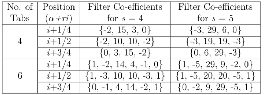
Table 3.1 DCTIF co-efficient values for tanh function approximation . . . 24 Table 3.2 Different tanh function implementations . . . 29 Table 4.1 Classification performance of DNN and SNN - FP: trained using
floating-point inputs and activations. Q: trained using quantized inputs and activations. QT2S: quantized inputs and activations trained using teacher-to-student approach. . . 38 Table 4.2 Comparison of several NN FPGA implementations on ZC706 for MNIST 43 Table 5.1 Performance comparison with existing FPGA-based DNN and CNN
accelerator designs . . . 64 Table 6.1 Accuracy comparison with existing decision tree approaches . . . 77 Table 7.1 Testing errors of Sinc, Sigmoid, MNIST and Cancer datasets using
different hyperbolic tangent approximations . . . 81 Table 7.2 Training errors of Sinc, Sigmoid, MNIST and Cancer using different
hyperbolic tangent approximations . . . 84 Table 7.3 Comparison of FPGA-based DNN and CNN accelerators for MNIST
LIST OF FIGURES
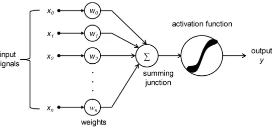
Figure 2.1 The basic components of an artificial neuron . . . 7
Figure 2.2 Non-linear activation functions (sigmoid, tanh and ReLU) . . . 7
Figure 2.3 Convolution neural network architecture . . . 12
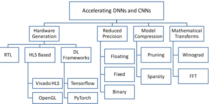
Figure 2.4 Different approaches of accelerating DNNs and CNNs on FPGAs . . . 18
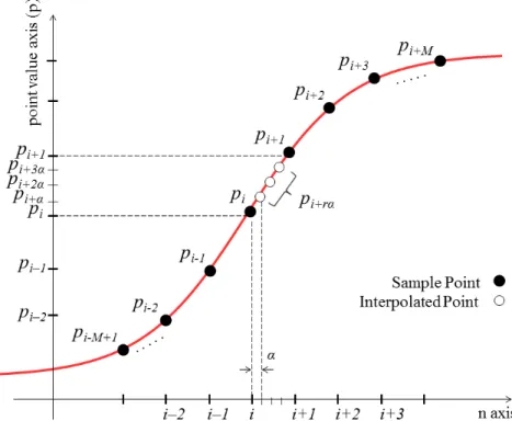
Figure 3.1 DCTIF approximation for tanh function . . . 23
Figure 3.2 Block diagram of the proposed tanh approximation . . . 25
Figure 3.3 The proposed DCTIF approximation architecture using 4 tabs, α = 1/4, s = 4 . . . . 25
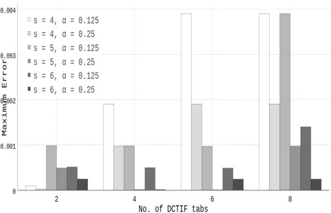
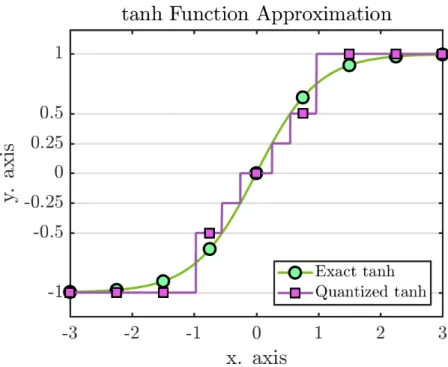
Figure 3.4 DCTIF tanh approximation accuracy vs no. of tabs, α value and the scaling parameter s using double floating-point data representation . 27 Figure 4.1 Quantizing the inputs to power-of-two values using stochastic rounding 34 Figure 4.2 Exact versus quantized tanh activation function . . . 36
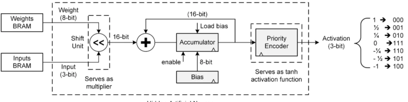
Figure 4.3 Proposed hidden artificial neuron architecture . . . 39
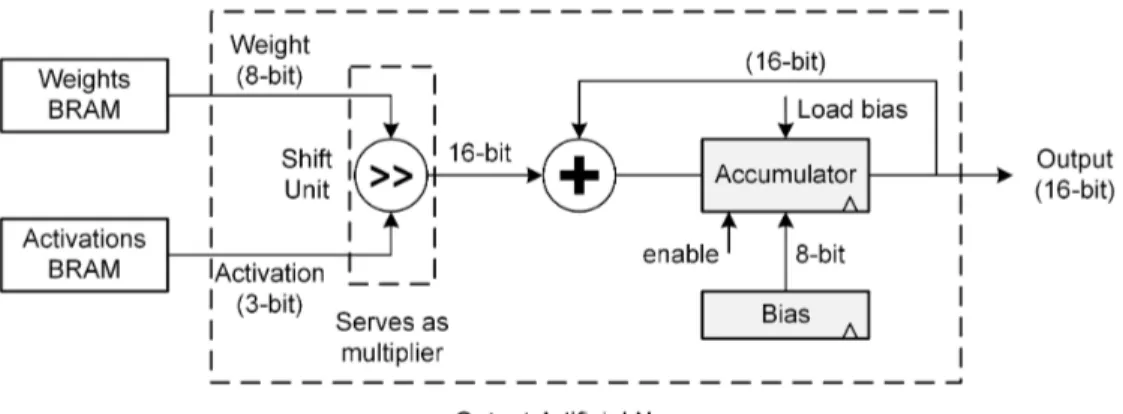
Figure 4.4 Proposed output artificial neuron architecture . . . 40
Figure 4.5 The testing platform of the proposed SNN overlay . . . 40
Figure 5.1 Real-valued artificial neuron vs binary artificial neuron . . . 49
Figure 5.2 Traditional BNN architecture with FC layers . . . 51
Figure 5.3 BNN architecture using a single FC layer with AND-OR gates . . . . 52
Figure 5.4 Overview of the POLYBiNN architecture and its use to classify FC applications and CIFAR-10 datasets . . . 54
Figure 5.5 POLYBiNN DT implementation in AND and OR gates . . . 55
Figure 5.6 Decision tree implementation as a SOP and a LUT . . . 55
Figure 5.7 Voting circuit implementation of POLYBiNN . . . 60
Figure 5.8 POLYBiNN HDL generation steps . . . 61
Figure 5.9 POLYBiNN performance analysis for MNIST and CIFAR-10 in terms of accuracy vs number of decision trees and number of splits for each class . . . 66
Figure 6.1 Overview of the POLYCiNN architecture with w windows and M classes 73 Figure 6.2 Local binary pattern encoding process . . . 73
Figure 6.3 Decision forests and decision fusion implementation of POLYCiNN . 75 Figure 6.4 Local binary pattern hardware implementation in POLYCiNN . . . . 75 Figure 6.5 POLYCiNN accuracy for the CIFAR-10, SVHN and MNIST datasets 78
Figure 7.1 Performance analysis of testing different DNNs architectures employing hyperbolic tangent activation function with different accuracies . . . 82
LIST OF SYMBOLS AND ACRONYMS
AN Artificial Neuron
ANN Artificial Neural Network
ASIC Application-Specific Integrated Circuit AdaBoost Adaptive Boosting
BNN Binary Neural Networks
BWN Binary Weights Neural Networks CNN Convolutional Neural Networks CPU Central Processing Unit
DCTIF Discrete Cosine Transform Interpolation Filter DF Decision Forests
DI Downsampled Image DMA Direct Memory Access DNN Deep Neural Network DSP Digital Signal Processing DT Decision Tree
EIE Efficient Inference Engine FANN Fast Artificial Neural Network FC Fully Connected
FFT Fast Fourier Transform
FINN Fast, Scalable Binarized Neural Network Inference FLOPS Floating Point Operations Per Second
FPGA Field Programmable Gate Array FPS Frames Per Second
GOPS Giga Operations Per Second GPU Graphical Processing Unit HDL Hardware Description Language HLS High-Level Synthesis
LBP Local Binary Pattern LSTM Long Short-Term Memory LUT Look-Up Table
MAC Multiply and Accumulate MLP Multi-Layer Perceptron NN Neural Network
NoC Network-on-Chip PL Programmable Logic PR Processing Region PS Processing System PWL Piecewise Non-Linear RAM Random Access Memory RNN Recurrent Neural Network
RSSI Received Signal Strength Indicator RTL Register Transfer Logic
ReLU Rectified Linear Unit
SNN Single hidden layer Neural Network SOP Sum-of-Product
SVM Support Vector Machine TOPS Tera Operations Per Second TPU Tensor Processing Unit
CHAPTER 1 INTRODUCTION
Machine learning is a field of artificial intelligence where computer algorithms are used to autonomously learn from data. Machine learning algorithms have been ubiquitous in several applications such as objects classification [1], pattern recognition [2] and regression problems [3]. Machine learning started early in 1950 when Alan Turing developed the Turing test to determine if a computer has real intelligence. The test is about fooling a human into believing that he/she had a natural text language conversation with another human while it is a machine. This machine is mainly designed to generate human-like responses. In 1952, Arthur Samuel wrote a computer learning program which was the game of checkers. A big step in the field of machine learning occurred when Frank Rosenblatt designed the first neural network for computers which simulates the thought processes of the human brain in 1957. Hence, the nearest neighbor algorithm was developed in 1967 that allows computers to recognize very basic patterns. In 1985, Terry Sejnowski developed NetTalk, which is a neural network that learns to pronounce words the same way a baby does. The power of machine learning started to appear when IBM’s Deep Blue computer beat the world champion at chess in 1997. Lately, the term deep learning started to appear. Deep learning offers new algorithms that can be used to let computers see and distinguish objects and text in images and videos using deep models with a large number of parameters. All in all, the latest technological advancements in machine learning approaches paved the way for new exciting and complex applications [4].
1.1 Overview
Artificial Neural Network (ANN) is one of the machine learning algorithms that achieves high performance in a diversity of applications. Usually the end user iteratively modifies the ANN’s architecture to better represent the provided examples and generalize to new data. ANNs consist of an input layer, a few hidden layers and an output layer. Each layer has a number of Artificial Neurons (ANs) that receive signals from inputs or other neurons and compute the weighted-sum of their inputs. Thereafter, an activation function is applied on the weighted-sum of each AN in order to introduce non-linearity into the network. Ten years ago, although there was no real restriction on the number of hidden layers in a Neural Network (NN), having more than two or three hidden layers was impractical in terms of computational complexity and memory access [5]. The main reason behind this is that the
existing Central Processing Units (CPUs) at that time were spending weeks or months to train a deep model.
Recently, deep learning has introduced deep models such as Deep Neural Networks (DNNs) and Convolutional Neural Networks (CNNs) where large numbers of hidden layers are used [4]. The deep models with many hidden layers usually achieve better performances than NNs especially at complex applications [6]. There have been attempts to address why DNNs usually outperform NNs in terms of accuracy [6]. One reason is that DNNs usually expand traditional NNs to a large scalable network with larger capacity of neurons and hidden layers [6]. In other words, deep models have the ability to learn more complex functions than simple NNs [7]. In the case of CNNs, they are trained to extract representative features from their inputs through several non-linear convolutional layers. Consequently, DNNs and CNNs achieve better performance than NNs in terms of classification accuracy.
Hardware accelerators played a major role in the development process of machine learning algorithms. Traditionally, CPUs with limited cores are insufficient in executing deep learn-ing models. Nowadays, hardware accelerators have massive computational resources and are capable of processing data faster. The success of deep machine learning models is massively linked to the development of parallel Graphical Processing Units (GPUs). GPUs brought a paradigm shift in reducing the computational time of the execution process of the training and inference processes of deep models. Although GPUs give developers the opportunity to use deeper models and train these models with more data, the complexity of some deep models exceeds the computational abilities of existing GPUs [8]. Moreover, GPUs consume high power which is a problematic for battery-powered devices. In addition, the high power consumption of GPUs limits the number of processors that can be used to improve GPUs’ performance in terms of throughput. Therefore, more efficient specialized hardware acceler-ators for DNNs are highly desired [8].
Application Specific Integrated Circuits (ASICs) are dedicated hardware for a specific ap-plication where both area and performance are well optimized. Although ASICs achieve good performance in terms of computational time, they are dedicated for specific applica-tions and have low level of configurability, and their time to market process is long. Field Programmable Gate Arrays (FPGAs) are hardware logic devices that have different amount of computational and memory resources that can be reconfigured to meet the requirements of several applications. FPGAs can be used to prototype ASICs with the intention of being replaced in the final production by the corresponding ASIC designs. However, FPGAs can achieve throughputs close to ASICs. In addition, the time-to-market of FPGA implementa-tions is significantly shorter than for ASIC implementaimplementa-tions. This is mainly because that,
unlike ASICs, FPGAs are not fully custom chips. So, no layouts, masks and manufacturing steps are required for an FPGA implementation. It is all about compiling the Hardware Description Language (HDL) code of the implementation on the target FPGA device. The manual intervention of the complex processes like placement, routing and time analysis in FPGA implementations is less than in ASIC. That is why the time-to-market of FPGA im-plementations is shorter than ASIC imim-plementations, and FPGAs are used in accelerating several complex applications.
1.2 Problem Statement
Deep learning hardware accelerators that score high on the 3Ps - Performance, Programma-bility and Power consumption - are highly desired. FPGAs achieve good performance in the 3Ps, but they have not been widely used for accelerating deep learning models com-pared to GPUs. The limited computation and memory resources of FPGAs might be the reason why they have not been used in accelerating deep learning applications. Moreover, the ease of the process of using GPUs over FPGAs in accelerating deep learning applica-tions is another reason. One motivation of the present work is to thus improve the mapping and scheduling of deep learning models such as DNNs and CNNs on current FPGAs within the available resource and external memory bandwidth constraints. Another motivation is the dearth of software libraries, frameworks and template-based compilers that can help de-velopers transform their high-level description of a deep learning architecture to a highly optimized FPGA-based accelerator with limited hardware design expertise. In this work, these motivations have led us to address three problems.
Firstly, we consider the problem of realizing a precise implementation of Fully Connected (FC) DNNs in FPGAs. This implementation entails a large number of additions and multi-plications that would badly increase the overall resources required for implementing a single AN with its non-linear activation function, and a fully parallel DNN. In addition, the pro-cess of describing a DNN for FPGA implementation often involves HDL modeling, for which designer productivity tends to be lower. These concerns must be addressed before FPGAs can become as popular as GPUs for DNN implementation.
Secondly, we consider the problem of implementing FC Binary Neural Networks (BNNs) in FPGAs. Recent works on compressing deep models have opened the door to implement deep and complex models in FPGAs with limited computational and memory resources. Moreover, reducing the precision of the data representation of DNN parameters from double floating-point to fixed-floating-point and binary representation proved efficient in terms of performance and compression. Although BNNs drastically reduce hardware resources consumption, complex
BNN models may need more computational and memory resources than those available in many current FPGAs. Therefore, optimization techniques that efficiently map BNNs to hardware are highly desired.
A third problem is how to realize efficient CNNs in FPGAs for solving classification problems. CNNs achieve state-of-the-art accuracy in many applications, however they have weaknesses that limit their use in embedded applications. A main downside of CNNs is their compu-tational complexity. They typically demand many Multiply and Accumulate (MAC) and memory access operations in both training and inference. Another drawback of CNNs is that they require careful selection of multiple hyper-parameters such as the number of con-volutional layers, the number of kernels, the kernel size and the learning rate. Consequently, other classifiers that suit the nature of FPGAs and achieve acceptable classification accuracy are worthy of exploration.
1.3 Research Contributions
The main objective of this work is to design and implement an efficient FPGA-based ac-celerators for DNNs and CNNs with the aim to achieve comparable performance as CPU and GPU-based accelerators and high throughput with high-level of design simplicity and flexibility. This section reviews the different contributions of this thesis. These contributions represent solutions to the problems detailed in section 1.2.
First, we propose a high precision approximation of the non-linear hyperbolic tangent acti-vation function while using few computational resources. We also study how the accuracy of the hyperbolic tangent activation function approximation changes the performance of differ-ent DNNs. The proposed approximation is configurable and its parameters can be chosen to trade off the accuracy and the overall circuit complexity. Moreover, it can be used for other activation functions such as sigmoid, sinusoid, etc. The proposed approximation achieves al-most 3× better precision than previous works in the literature while using a similar amount of computational resources and a small amount of memory. This work was published in the ACM/SIGDA International Symposium on Field-Programmable Gate Arrays in 2017 [9] entitled “Accurate and Efficient Hyperbolic Tangent Activation Function on FPGA using the DCT Interpolation Filter”, and in IEEE Annual International Symposium on Field-Programmable Custom Computing Machines in 2017 in [10] entitled “A configurable FPGA Implementation of the Tanh Function using DCT Interpolation”.
Second, we propose a single hidden layer NN multiplication-free overlay architecture with DNN-level performance. The overlay is cheap in terms of computations since it avoids
mul-tiplications and floating-point operations. Moreover, it is user friendly especially for users with no FPGA experience. In a couple of minutes, the user can configure the overlay with the network model using a traditional C code. This work was published in the International Conference on ReConFigurable Computing and FPGAs (ReConFig) in 2018 [11] entitled “An Efficient FPGA-based Overlay Inference Architecture for Fully Connected DNNs”.
Third, we propose POLYBiNN, an efficient FPGA-based inference engine for DNNs using decision trees, which are binary classifiers by nature. POLYBiNN is a memory-free inference engine that drastically cuts hardware costs. We also propose a tool for the automatic gener-ation of a low-level hardware description of the trained POLYBiNN for a given applicgener-ation. This work was published in the IEEE Conference on Design and Architectures for Signal and Image Processing (DASIP) in 2018 [12] entitled “POLYBiNN: A Scalable and Efficient Com-binatorial Inference Engine for Neural Networks on FPGA” and got best paper award, and in Journal of Signal Processing Systems in 2019 [13] entitled “POLYBiNN: Binary Inference Engine for Neural Networks using Decision Trees”.
Fourth, we propose POLYCiNN, a classifier inspired by CNNs and decision forest classifiers. POLYCiNN migrates CNN concepts to decision forests as a promising approach for reducing both execution time and power consumption while achieving acceptable accuracy in CNN applications. POLYCiNN can be efficiently mapped to simple and densely parallel hardware designs since each decision tree is implemented in a single Look-Up Table. This work was accepted for publication in the IEEE Conference on Design and Architectures for Signal and Image Processing (DASIP) in 2019 [14] entitled “POLYCiNN: Multiclass Binary Inference Engine using Convolutional Decision Forests”.
1.4 Thesis Organization
This thesis is organized as follows. Chapter 2 introduces the basic concepts of NNs and deep learning models. Moreover, it provides a review of recent literature about the dif-ferent software and hardware acceleration approaches of DNNs and CNNs. We detail the contributions of this work in the four subsequent chapters. In chapter 3, we present a con-figurable FPGA implementation of the tanh activation function. In chapter 4, we describe an efficient FPGA-based overlay inference engine for DNNs. We introduce POLYBiNN, a binary inference engine for DNNs in chapter 5. Chapter 6 presents POLYCiNN, a multiclass binary inference engine for CNN applications. Chapter 7 gives a general discussion about the proposed implementations. Chapter 8 concludes this thesis and outlines future research directions.
CHAPTER 2 BACKGROUND AND LITERATURE REVIEW
In this chapter, we provide background information and a literature review on DNNs and CNNs. We begin by giving the basic principles of NNs in terms of their architectures and working theorems. We describe the concept of deep learning and present its different models and applications. We also review the literature regarding the different implementation ap-proaches of DNNs and CNNs. Finally, we discuss the pros and cons of the different hardware acceleration platforms for DNNs and CNNs.
2.1 Artificial Neural Networks
ANNs are computational models inspired by the principles of computations performed by the biological NNs of human brains [15]. Nowadays, several applications in different domains use ANNs, for example, signal processing, image analysis, medical diagnosis systems, and finan-cial forecasting [15]. In these applications, the main role of ANNs is either classification or functional approximation (regression) [3]. In classification, the main objective is to provide a meaningful categorization or proper classification of input data. In functional approximation, ANNs try to find a functional model that smoothly approximates the actual mapping of the given input and output data.
2.1.1 Neural Network Components
ANNs consist of an input layer, a number of hidden layers and an output layer. Each layer is composed of a number of ANs that are considered the basic elements of NNs. These ANs receive signals from either inputs or other neurons and compute the weighted-sum of their inputs, as shown in Fig. 2.1. Theoretically, each AN serves as a gate and uses an activation function to determine whether to fire and produce an output from its input or not [3]. Usually, activation functions are applied in order to introduce non-linearity into the network.
An activation function is a transfer function that takes the weighted-sum of a neuron and transfers it to an output signal. Fig. 2.2 shows the most common activation functions that are used in different NN applications. Generally, NNs activation functions can be placed into two main categories: 1) sigmoidal and 2) non-sigmoidal activation functions [16]. The term sigmoidal function refers to any function that takes an S-shape curve. The sigmoid and hyperbolic tangent functions are bounded, differentiable and continuous sigmoidal functions.
Figure 2.1 The basic components of an artificial neuron
Non-sigmoidal activation functions such as Rectified Linear Unit (ReLU) are not bounded and achieve better performance than sigmoidal functions in many applications [16]. Moreover, non-sigmoidal functions are computationally efficient as they require a simple comparison between two values. They also have a sparse representation in their output values.
An artificial neuron, or perceptron, can separate its input data into two classes in a linear relation [17]. In order to solve non-linear complex functions, several ANs are used in multiple layers where the outputs of the ANs of one layer are connected to the inputs of the next layer. A Multi-Layer Perceptron (MLP) is a feed-forward NN that consists of an input layer of ANs, followed by two or more layers of ANs with a final output layer. The term feed-forward indicates that the network feeds its inputs to the hidden layers towards the output layer in only one direction. The performance of a NN for a given application depends on the associated weights of its ANs. Those weights are determined through training the network on the given data iteratively. Once NNs are well trained and tested on a sufficient amount
of data in order to generalize their classification or functional approximation surface, their models can be applied on new data.
2.1.2 Model Selection
The objective of model selection process in NNs is to find the network architecture with the best generalization properties, which minimize the error on the selected samples (training and validation samples) of the dataset. This process defines the number of layers of the network, number of ANs per layer, the interconnections, type of activation function, etc. These settings are called hyper-parameters that control the behaviour of the corresponding network. Conceptually, hyper-parameters can be considered orthogonal to the learning model itself in the sense that, each network architecture with a set of hyper-parameters is considered a hypothesis space. The training process of that network optimizes the hypothesis within that space. For example, we can think of model selection for a given application as the process of choosing the degree of the polynomial that best represents the given data of this application. Once the polynomial degree is determined, adjusting the parameters of the polynomial is considered as the optimization of the hypothesis.
All these hyper-parameters, alongside with learning rate, epochs, etc. must be chosen before training and are picked manually based on experience [17]. The major drawback of this strategy is the difficulty of reproducing the results as this optimization strategy takes time and depends on the experience of the developer [22]. There are some other automatic strategies such as grid search [23] and random search [22], however they do not perform as well as manual optimization especially in deep models [22].
2.1.3 Training Artificial Neural Networks
NNs can be classified into three main types according to how they learn: supervised, semi-supervised and unsemi-supervised learning networks. In semi-supervised learning, the aim is to discover a function that approximates the true function of a given training set that has sample input-output pairs [18] with a high degree of accuracy. In this case the input-output value of each input is available and the labeled examples of the training set serve to supervise network training. On the other hand, unsupervised NNs learn patterns of the input data even though no explicit feedback is supplied. These networks are often used in clustering applications [18]. Semi-supervised NNs have few labeled examples and a large collection of unlabeled examples. Semi-supervised NNs use both types of examples to learn the best classification or clustering model of the given data.
In supervised learning, training NNs is mainly about adjusting the network weight and bias values to minimize the loss function [18]. The loss function is defined as the amount of utility lost by approximating a model for the given data to its correct answer. In other words, the loss function measures how the predicted model fits the data. Therefore, adjusting the weight and bias values can be addressed by a hill-climbing algorithm that follows the gradient of the loss function to be optimized. Although there are complex techniques to initialize the weight and the bias values, random weight values and zero bias values are often used [20].
Generally, the error back-propagation algorithm is the most common technique for training ANNs [17]. It consists of two paths through the ANN layers: a feed-forward and a back-propagation paths. First, in the feed-forward path, the network takes the input values of a single training sample (stochastic) or a number of samples (mini-batch) or all training samples (batch). These inputs are multiplied by the initialized weight values and then the weighted-sum values are calculated and passed through the pre-defined activation function of each AN till the output layer. In the feed-forward path, the weights and bias values are fixed and are not updated. Once the outputs appear at the output layer, the loss function is computed by subtracting the output layer response from the expected output vector. In the back-propagation path, the loss function value is back propagated through the different layers of the network to update the weights and biases. The gradient descent algorithm [21] computes the gradient of the loss function with respect to each weight and bias value at the different layers. The gradient values along with the learning rate are used to update the weights and biases of the model. The feed-forward and back-propagation paths are repeated several times, called epochs, until the network is trained according to the training algorithm’s constraint.
When training NNs, it is crucial to have separate training, validation and test sets [19]. The training set usually represents 70% of the overall data and it is used to train the network fitting the model to the given data. The validation set, which usually represents 15% of the data, is used to tune the ANN’s hyper-parameters. It also prevents overfitting during training by performing early stopping. The key point of early stopping is to find the weight values and biases during training for which the validation set curve begins to deteriorate [19]. In other words, when the classification performance of the validation dataset meets the requirements, the training algorithms stops updating the weigh and bias value. After training the model, the test set is used to assess the generalization of the trained model on new data.
2.2 Deep Learning
Deep learning is a form of machine learning that uses multiple transformation steps in or-der to discover representative features or patterns in the given data [19]. The word deep refers to the fact that the outputs are derived from the inputs by passing through multiple layers of transformations. In deep learning, the models jointly learn the most representa-tive complex features across the different layers of the network. Recently, impressive results were achieved in speech recognition and computer vision applications using different machine learning models such as DNNs, CNNs, and Recurrent Neural Networks (RNNs) [4, 19].
2.2.1 Deep Learning into Action
The use of deep learning models is not a novel concept especially that it has been proposed since developing NNs. However, deep models were out of reach as their computational com-plexity were exceeding the available computational platforms capabilities [5]. Three facts have facilitated the resurgence of deep learning models; a) the availability of large datasets, b) the development of faster and parallel computation units and c) the development of new sparsity, regularization and optimization machine learning techniques [4]. Nowadays, re-searchers and organizations can collect massive amount of data that can be used to train deep models with many parameters. In addition, techniques such as dropout and data aug-mentation [24] can generate more training samples from a small dataset. On the other hand, the availability of high-speed computational units such as GPUs and cloud computing are valued in deep learning since they can adequately handle large amounts of computational work quickly. Consequently, the revolution of deep learning has been enabled by the existing hardware accelerators.
2.2.2 Deep Neural Networks
NNs have been considered standard machine learning techniques for decades, however DNNs with higher capacity that have a larger number of hidden layers achieve better performance compared to NNs [6]. DNN is considered the basic model of deep learning that performs computations on deep FC layers. Usually, DNNs use the same activation functions used in NNs such as sigmoid and tanh. However, for DNNs, ReLU activation function is favorable in some applications since it outputs zero for all negative inputs. This is often desirable because there are fewer computations to perform and this results in concise DNN models that achieve more generalization towards the corresponding application and more immune
to noise. Training DNNs is exactly the same process as training NNs with more number of hidden layers using the back-propagation algorithm.
2.2.3 Convolution Neural Networks
CNNs are a special kind of feed-forward networks that have achieved success for image analysis, pattern recognition and image based classification applications. CNNs process the given data in the form of arrays containing pixel values, for example a color RGB image. A typical CNN, as shown in Fig. 2.3, consists of a series of stages where each stage has three layers: a convolution layer, an activation layer and a pooling layer.
The convolution layer applies learnable filters on small spatial regions of the input image. The output of each filter is called a feature map. This process extracts the most important and representative features of the input image. Once an image has been filtered, the output feature maps are passed through a non-linear activation function in the second layer. Usually, the ReLU activation function achieves good performance when working with images [1, 4]. Finally, a pooling or a decimation layer is applied which subsamples the output feature maps from the activation layer. The main task of pooling layers is to reduce the computational complexity of the network and generalize the model more to achieve good performance of the testing dataset. The subsampling process usually uses the max operation that activates a feature if it is detected anywhere in the pooling zone. A few FC layers before the output layer link all the extracted features together and classify an input sample.
2.3 DNN and CNN Acceleration
GPUs, custom ASICs and FPGAs have been the main approaches for accelerating the training and the inference of a deep model [8, 25]. Not only hardware accelerators, but algorithmic and software approaches have been used as well to reduce DNN and CNN computations.
2.3.1 Algorithmic and Software Approaches
There are some algorithmic trends in accelerating deep models [25]: using more compact data types, taking advantage of sparsity, models compression and mathematical transforms.
Recently, it has been shown that deeper models can achieve higher accuracies than simple models [2]. However, deeper models require more computations and memory accesses to perform their tasks. For example, ResNet [26] has significantly increased the top-5 accuracy on the Imagenet [27] dataset to 96.4% compared to 84.7% using AlexNet [1]. However,
Figure 2.3 Con v olution neural net w ork arc hitecture
ResNet uses 152 layers and requires 11 B Floating Point Operations Per Second (FLOPS) while AlexNet has only eight layers and requires 1.5B FLOPS. The computational efficiency of the network can be improved by using more compact data types. Usually, double floating-point data representation is used in the training process of DNNs. However, many researchers have shown that it is possible to train and perform the inference process using fixed-point data representation [6, 28–30]. Moreover, more compact data representations such as BNNs [30] have achieved performances comparable to fixed and floating-point data representations. BNNs can significantly reduce network parameter storage. In addition, the multiply and the accumulation processes are replaced by boolean operators which dramatically cut the required computations of the network.
Sparsity is another trend in DNNs that reduces their computational complexity in the training and the inference stages. Albreicio et al. [31] reported that more than 50% of the AN values of some popular DNNs are zeros. Moreover, the ReLU function, which is the most commonly used activation function [4], helps in building sparse activations since it outputs zero for negative inputs. Computations on such zero-valued activations are unnecessary. This results in transforming the traditional matrix multiplications to sparse matrix multiplications that require fewer operations than dense matrix [25]. Furthermore, Han et al. [28] proposed a pruning technique that zeros out the non-important neurons to generate a sparse matrix. This reduces the computational complexity of the network while maintaining comparable accuracy. Moreover, several compression techniques of DNNs have been proposed such as weight sharing [28] and hashing function [32].
Several software libraries have been developed for designing, simulating and evaluating DNNs and CNNs. Most of these libraries allow users to deploy their models to different hardware platforms i.e. CPUs and GPUs. Some popular examples of open source NN libraries are Fast Artificial Neural Network (FANN) developed in C [34], OpenNN developed in C++ [35] and OpenCV library for NNs developed in C/C++ [36]. Moreover, open source software platforms for machine learning, e.g. Tensorflow [37] and PyTorch [38] can realize DNN and CNN applications. Although GPUs are powerful hardware accelerators mainly designed for image and video processing application, they can also be used to accelerate any parallel single instruction multiple data application which exactly fits to NN applications. GPUs are working in the sense that the users have to translate their program into an explicit graphics language, e.g., OpenGL. However, NVIDIA introduced CUDA [39], a C/C++ language that enables more straightforward programming on the parallel architecture of a GPU. Therefore, we consider GPUs as a software approach as most of the discussed software libraries e.g. Tensorflow, PyTorch and Matlab deep learning library [40] are compatible with GPUs without any required modifications by the users.
DNNs are represented in software as control programs that operate on memory locations containing the inputs and the output data of each AN. These ANs are connected through pointers that are flexible. The execution time of DNN applications with software approaches depends on the processor performance of the host computing platform. Moreover, the in-struction set of these processors are not specific for DNN applications. Therefore, the major drawback of DNN software-based implementations is the slow execution process [33]. More-over, the execution time is affected by the memory access latency in order to read/write the required data/result, respectively. Therefore, hardware accelerators are highly desired for DNN and CNN applications [8].
2.3.2 GPU Acceleration
GPUs are often preferred for computations that exhibit regular parallelism and demand high throughput. In addition, GPUs are high-level language programmable devices and their development process is accessible to most designers. Consequently, GPUs are popular in machine learning applications as they match the nature of these models [8] [17] [19]. Recently, GPUs offer increased FLOPS, by incorporating more floating-point units, on-chip RAMs, and higher memory bandwidth [25]. However, GPUs still face challenges in deep learning models such as handling irregular parallel operations. In addition, GPUs support only a fixed set of native data types and they do not have the ability to support other custom different data types. GPUs still cannot meet the performance requirements of several real-time machine learning applications [17] [41] [42]. It might take weeks or even months in order to train some DNN applications. In addition, GPUs usually consume a significant amount power which is problematic especially for mobile and embedded devices.
2.3.3 ASIC-based Acceleration
ASICs can optimize both area and performance for a given DNN application in a better way than FPGAs since they are specific for a given application. The main concerns when using NN ASIC accelerators are the time to market, the cost and the low-level of flexibility of the implementation. Han and colleagues [43] introduced a compression technique for DNN weights and also proposed skipping the computational activities of zero weights. They imple-mented their proposed Efficient Inference Engine (EIE) for DNNs on ASIC 45nm technology. On nine fully connected layers benchmark, EIE outperforms CPU, GPU and mobile GPU by factors of 189×, 13× and 307×, respectively. It also consumes 24,000×, 3,400× and 2,700× less energy than CPU, GPU and mobile GPU, respectively. Wang et al. [44] proposed a low power CNN on a chip by quantizing the weight and bias values. The proposed dynamic
quantization method diminishes the required memory size for storing the weight and bias values and reduces the total power consumption of the implementation.
Eyeriss by Chen et al. [45,46], which is an energy efficient reconfigurable CNN chip, uses 16-bit fixed point instead of floating data representation. The authors mapped the 2D convolution operations to 1D convolution across multiple processing engines. The Eyeriss chip provides 2.5× better energy efficiency over other implementations. The authors extended their work and proposed Eyeriss v2, which is a low-cost and scalable Network-on-Chip (NoC) design that connects the high-bandwidth global buffer to the array of processing elements in a two-level hierarchy [46]. This enables high-bandwidth data transfer and high throughput. Following Eyeriss chip, Adri et al. [47] proposed the YodaNN that uses binary weights instead of 16-bit fixed point data representation.
DianNao [48] is an ASIC DNN accelerator designed with a main focus of minimizing off-chip communication. The accelerator achieves up to 452 Giga Operations Per Second (GOPS) while consuming 485 mW and running at 980 MHz. The authors extended DianNao accel-erator to a multi-mode supercomputer for both DNN inference and training [49, 50]. The chip consumes 16 W while running at 600 MHz, and it allows the use of 16-bit precision for inference and 32-bit precision for training with minimal effect on accuracy. Cnvlutin [31] is an ASIC CNN accelerator that is designed to skip ineffectual operations in which one of the operands is zero. The authors reported 4.5% area overhead and 1.37 higher performance compared to DaDianNao [50] without any loss in accuracy.
To alleviate the limitations of fixed-bitwidth ASIC accelerators, Sharma et al. [51] proposed BitFusion, a dynamic bithwidth DNN accelerator with 16-bit fixed-point arithmetic compu-tational units that can be combined to create higher precision arithmetic units. Google’s Tensor Processing Unit (TPU) [52] is another ASIC inference accelerator that contains a 2D systolic matrix multiply unit that uses 8-bit fixed-point precision. It runs at 700 MHz and achieves a peak performance of 92 Tera Operations Per Second (TOPS). The TPU work has been extended to support both training and inference with a peak performance of 11.5 peta FLOPS for a single TPU [53].
2.3.4 FPGA-based Acceleration
Although FPGAs are used in accelerating many applications, they still have some disadvan-tages that might limit their roles in deep learning applications. One issue with FPGAs is that in terms of power consumption they consume more power than ASICs. In addition, there is no control over the power optimization in FPGAs which is not the case in ASICs. Another issue is that the design size is limited by the available resources of the target FPGA
device. Moreover, the synthesis, place and route processes of the design on FPGAs take time and these processes should be repeated after each new design.
There have been several attempts to implement both the feed-forward and back-propagation algorithms on FPGAs. Zamarano and his colleagues [54] implemented on FPGAs the back-propagation and feed-forward algorithms that are used in the training, the validation and the testing processes of NNs. They introduced a different AN representation by combining the ANs of the input and the first hidden layers in order to reduce the computational resources usage. Yu et al. [55] presented an FPGA-based accelerator for NNs, but it does not support variable network size and topology. Since memory capacities of FPGAs are limited, Park and his colleagues [56] proposed a NN accelerator on FPGA that uses 3-bit weights and a fixed point weight optimization in the training phase. This approach allows storing the NN weight values on the on-chip memory. This reduces the external memory access latency and speeds-up the overall implementation. Wang et al. [57] proposed a scalable deep learning accelerator unit on FPGA. It employs three different pipelined processing units: tiled ma-trix multiplication, part sum accumulation and activation function acceleration units. The proposed inference implementation achieves 36.1× speedup compared to current CPU im-plementations with reasonable hardware cost and lower power utilization on the MNIST dataset.
Zhang et al. [58] presented an analytical methodology for design space exploration on FPGA to find the design parameters that result in highest throughput within the given resource and memory bandwidth constraints for each convolutional layer separately. This work was extended to a multi-FPGA cluster instead of a single FPGA [59] that uses 16-bit fixed point precision. Li et al. [60] proposed a high performance FPGA-based accelerator for the inference of large-scale CNNs. They implemented the different layers to work concurrently in a pipelined structure to increase the throughput. In the fully connected layer, a batch based computing method is adopted to reduce the required memory bandwidth. The proposed implementation was tested by accelerating AlexNet, it can achieve a performance of 565.94 GOPS at 156 MHz. Targeting more flexible FPGA architectures, Ma et al. [61] presented a scalable RTL compilation of CNNs onto FPGA. They developed a compiler that analyzes a CNN structure and generates a set of scalable computing primitives that can accelerate the inference of the given CNN model. The authors tested their idea on accelerating AlexNet. On Altera Startix-V FPGA, the implementation achieves 114.5 GOPS. Recently, mathematical optimizations such as Winograd Transform and Fast Fourier Transform (FFT) have been used to decrease the number of arithmetic operations required when implementing DNNs and CNNs in FPGAs [62, 63].
Binary DNNs and CNNs have proposed using extremely compact 1-bit data types for both the weights and biases values [64]. This novel idea massively simplifies the computations of the weight-sums of ANs by replacing the matrix multiplications by XNOR and bit-counting operations. Umuroglu et al. [65] implemented a framework for fast scalable binarized NNs. They implemented the fully connected, pooling and convolution layers of the MNIST CNN on a ZC706 embedded FPGA platform consuming less than 25 W total system power. They re-ported 95.8% accuracy while processing 12.3M images per second of the MNIST CNN. More-over, Fraser et al. [66] demonstrated numerous experiments on binary NNs and a Framework for Fast, Scalable Binarized Neural Network Inference (FINN) in order to show the scalabil-ity, flexibility and performance of FINN on large and complex deep models. On the other hand, Alemdar et al. [67] implemented a fully connected ternary weight NN that trains the weights with only three values (-1, 0, 1). They reported that the proposed implementation processes 255K frames per second on the MNIST dataset.
Venieris et al. [68] introduced fpgaConvNet, a framework that takes a CNN model described in the C programming language and generates a Vivado High-Level Synthesis (HLS) hardware design. The framework employs a set of transformations that explore the performance-resource design space. Wei et al. [69] proposed another framework that generates a high-performance systolic array CNN implementation in FPGAs from a C program. Noronha et al. [70] proposed LeFlow, a tool that maps numerical computation models such as DNNs and CNNs written in Tensorflow to synthesizable hardware in FPGA.
FPGAs have advanced significantly in recent years by incorporating large on-chip RAMs, large amount of Look-Up Tables (LUTs) and Digital Signal Processing (DSP) slices for com-plex arithmetic operations. In addition, the off-chip memory bandwidth is also increasing with the integration of recent memory technologies. Moreover, the development process on FPGAs has become much easier using recent tools such Vivado HLS. Such tools allow C/C++ algorithms to be compiled and synthesized which made the development process easier to software developers. Hence, FPGAs have the opportunity to do increasingly well on the next-generation DNNs and CNNs as they become more irregular and use custom data types.
2.3.5 DNN and CNN Acceleration Summary
Figure 2.4 summarizes the four approaches of accelerating DNNs and CNNs detailed in section 2.3. The approaches can be classified into four major directions. The first approach employs different computational transforms to vectorize the implementations and reduce the number of arithmetic operations occurring during inference. The second approach is the compression
Figure 2.4 Different approaches of accelerating DNNs and CNNs on FPGAs
of the model and removing the unnecessary ANs and connections. The third approach is the use of reduced precision weights and activations without critically affecting DNN and CNN performances. The fourth approach is related to how to describe any DNN or CNN model on FPGA.
2.4 Summary and Research Objectives
The DNN and CNN acceleration approaches can be used separately or together to achieve the required performance for a given application on FPGAs. The two main approaches that are used to accelerate DNNs and CNNs on FPGAs are the reduced precision and the hardware generation. The reduced precision approach of DNNs and CNNs suits the nature of FPGAs especially when it comes to using binary precision. The hardware generation approach solves the difficulty of expressing DNN and CNN models in HDL. Recent FPGA-based CNN and DNN accelerators can outperform GPUs in terms of performance while consuming less power but they still pose special challenges. One issue is that FPGAs have limited or costly computational capabilities, which hinders the realization of large DNNs and CNNs. Another challenge is that the synthesis, place and route processes can take an unacceptable amount of time. In addition, the process of describing DNNs or CNNs on FPGAs often involves modeling in a HDL, for which designer productivity tends to be lower.
The existing high level synthesis tools typically generate a non-optimized hardware solutions for DNNs and CNNs. On the other hand, expressing DNNs and CNNs with Register Transfer Logic (RTL) take a long development round. Therefore, in this thesis, we focus on the reduced precision and hardware generation approaches.
The main goal of this thesis is to propose a designer friendly and efficient FPGA-based inference architectures suitable for DNN and CNN applications with varied computational and memory requirements. In order to reach our goals, the following specific objectives are identified:
• Propose adequate optimized hardware architectures of DNNs and CNNs in FPGAs. The proposed architectures should satisfy precise performance while consuming few computations and memory.
• Develop tools able to generate optimized low-level HDL description automatically for the proposed architectures.
• Simulate, implement, test and evaluate the proposed architectures to assess their per-formance, and compare them to the existing works.
CHAPTER 3 ARTICLE 1: A CONFIGURABLE FPGA IMPLEMENTATION OF THE TANH FUNCTION USING DCT
INTERPOLATION
Authors: Ahmed M. Abdelsalam, J.M. Pierre Langlois and F. Cheriet
Published in: IEEE 25th Annual International Symposium on Field-Programmable Custom Computing Machines (FCCM) 2017 [10]
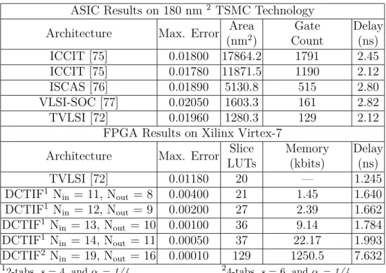
Abstract–Efficient implementation of non-linear activation functions is essential to the implementation of deep learning models on FPGAs. We introduce such an implementation based on the Discrete Cosine Transform Interpolation Filter (DCTIF). The proposed interpolation architecture combines simple arithmetic operations on the stored samples of the hyperbolic tangent function and on input data. It achieves almost 3× better precision than previous works while using a similar amount computational resources and a small amount of memory. Various combinations of DCTIF parameters can be chosen to trade off the accuracy and the overall circuit complexity of the tanh function. In one case, the proposed architecture approximates the hyperbolic tangent activation function with 0.004 maximum error while requiring only 1.45 kbits BRAM memory and 21 LUTs of a Virtex-7 FPGA.
3.1 Introduction
Deep Neural Networks (DNN) have been widely adopted in several applications such as ob-ject classification, pattern recognition and regression problems [4]. Although DNNs achieve high performance in many applications, this comes at the expense of a large number of arithmetic and memory access operations [71]. Therefore, DNN accelerators are highly de-sired [8]. FPGA-based DNN accelerators are favorable since FPGA platforms support high performance, configurability, low power consumption and quick development process [8].
DNNs consist of a number of hidden layers that work in parallel, and each hidden layer has a number of Artificial Neurons (AN) [4]. Each neuron receives signals from other neurons and computes a weighted-sum of these inputs. Then, an activation function of the AN is applied on this weighted-sum. One of the main purposes of the activation function is to introduce non-linearity into the network. The hyperbolic tangent is one of the most popular non-linear activation functions in DNNs [4]. Realizing a precise implementation of the tanh function in
hardware entails a large number of additions and multiplications [72]. This implementation would greatly increase the overall resources required for implementing a single AN and a fully parallel DNN. Therefore, approximations with different precisions and resources are generally employed [8].
There are several approaches for the hardware implementation of the tanh function based on Piecewise Linear, Piecewise Non-Linear (PWL), Lookup Table (LUT) and hybrid methods. All of these approaches exploit the fact that the tanh function is negatively symmetric about the Y-axis. Therefore, the function can be evaluated for negative inputs by negating the output values of the same corresponding positive values and vice versa. Armato et al. [73] proposed to use PWL which divides the tanh function into segments and employs a linear approximation for each segment. Zhang and his colleagues [74] used a non-linear approxima-tion for each segment. Although both methods achieve precise approximaapproxima-tions for the tanh function, this comes at the expense of the throughput of the implementation. LUT-based approximations divide the input range into sub-ranges where the output of each sub-range is stored in a LUT. Leboeuf et al. [75] proposed using a classical LUT and a Range Addressable LUT to approximate the function. LUT-based implementations are fast but they require more resources than PWL to achieve the same accuracy. Therefore, most of the existing LUT-based methods limit the approximation accuracy to the range [0.02, 0.04].
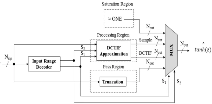
Several authors have observed that the tanh function can be divided into three regions: Pass Region, Processing Region (PR) and Saturation Region as shown in Fig. 3.1. The tanh function behaves almost like the identity function in the Pass Region, and its value is close to 1 in the Saturation Region. Some hybrid methods that combine LUTs and computations were used to approximate the non-linear PR. Namin and his colleagues [76] proposed to apply a PWL algorithm for the PR. Meher et al. [77] proposed to divide the input range of the PR into sub-ranges, and they implemented a decoder that takes the input value and selects which value should appear on the output port. Finally, Zamanloony et al. [72] introduced a mathematical analysis that defines the boundaries of the Pass, Processing and Saturation Regions of the tanh function based on the desired maximum error of the approximation.
In this paper, we propose a high-accuracy approximation using Discrete Cosine Transform Interpolation Filter (DCTIF) [78]. This paper is based on a previously presented abstract [9]. The proposed approximation achieves higher accuracy than the existing approximations, and it needs fewer resources than other designs when a high precision approximation is required. The rest of the paper is organized as follows: the operation principle of the proposed DCTIF approximation is described in Section 3.2. In Section 3.3, an implementation of the