What Optech's Bathymetric LiDAR Sees Underwater
Bernard Long, Antoine Cottin, Antoine Collin
Institut National de la Recherche Scientifique Eau, Terre et Environnement
Québec, Canada [email protected]
Abstract— This article presents early results of the FUDOTERAM project using bathymetric LiDAR data acquired with the SHOALS-3000, the latest bathymetric LiDAR system from Optech. The survey area is in the coastal zone along the northern shore of Chaleurs Bay, in the western Gulf of St. Lawrence, Canada. The project aimed to apply the SHOALS-3000 to geological mapping, sedimentary process monitoring and marine habitat mapping. This paper focuses on the sedimentological part of the study and presents the early raw data obtained to produce a bottom type classification based on some simple parameters, roughness, slope angle and direction. Two methods are evaluated for analysis of the SHOALS-3000 waveforms, the Moment Method and the Gaussian Mixture Model, and the latter is used as an approach to model the bottom type signal.
Keywords: LiDAR, bathymetry, seabed classification I. INTRODUCTION
The shallow coastal seabed in depth less than 10 m remain a challenging environment for monitoring and mapping due to difficult access and the lack of suitable sensors. The concentration of human population and economic activity in the dynamic coastal zone creates an important need for such information to support effective and sustainable management. The FUDOTERAM project aimed to develop an efficient management tool through the use of a bathymetric LiDAR system, the SHOALS-3000. This paper describes the application of this system to geological mapping and sedimentary process monitoring of the coastal zone.
II. MATERIALS AND METHODS
A. Study site
For this project we chose a survey area along the northern shore of the Baie des Chaleurs in eastern Québec, Canada. Two sites were selected in part on the basis of the wave energy difference. Paspébiac is exposed to high energy waves, while the wave energy at Bonaventure is more modest, allowing the development of various sedimentary facies and processes as well as a variety of biological environments. The local bedrock is a red Paleozoic sandstone with some conglomerates. Sandy spits, barrier beaches and coastal dunes are formed of sediment derived from the bedrock or other deposits from the Pleistocene ice age. In this paper, we focus on the Paspébiac area.
B. The SHOALS-3000 sytem
The SHOALS-3000 (Scanning Hydrographic Operational Airborne LiDAR Survey) is a bathymetric LiDAR that uses a pulsed Nd:YAG laser head, generating a fundamental near infra-red (1064 nm) beam and a frequency-doubled blue-green (532 nm) beam. The laser is pulsed at 3 kHz (Table 1). The laser’s scan shape is designed to produce a semi-arc on the ground that ensures a constant angle to the nadir (20° ahead on the aircraft heading). The laser footprint diameter is 2 m. The pulse width is 6 ns with a total emitted energy of 7.5 mJ. The return signals, e.g. the waveforms, are digitized into 1 ns bins, which correspond to a vertical resolution of 15 cm. Four channels are recorded - shallow and deep blue-green, near infra-red and the Raman. The two blue-green channels measure the shallow (1-12 m) and the deep (≥7 m) bathymetry. The
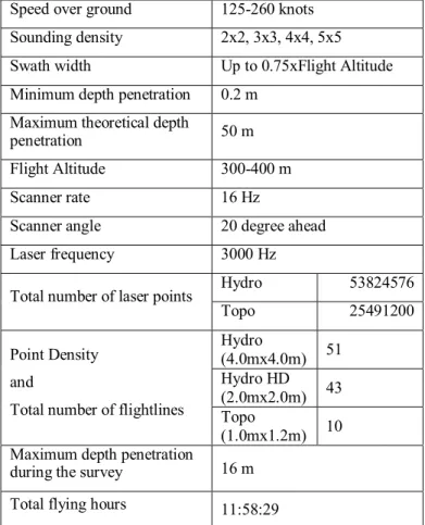
Speed over ground 125-260 knots Sounding density 2x2, 3x3, 4x4, 5x5 Swath width Up to 0.75xFlight Altitude Minimum depth penetration 0.2 m
Maximum theoretical depth
penetration 50 m
Flight Altitude 300-400 m
Scanner rate 16 Hz
Scanner angle 20 degree ahead Laser frequency 3000 Hz
Hydro 53824576 Total number of laser points
Topo 25491200 Hydro (4.0mx4.0m) 51 Hydro HD (2.0mx2.0m) 43 Point Density and
Total number of flightlines Topo
(1.0mx1.2m) 10 Maximum depth penetration
during the survey 16 m Total flying hours 11:58:29
Table 1. SHOALS-3000 specifications and survey statistics.
infra-red channel is used to locate the water surface and as an indicator of ground type (land or water) for auto-switch between hydrographic and topographic mode. The Raman channel is use to locate the surface, mainly in case of lambertian reflection from a very flat sea surface. For each pulse, this system records the elevation data through analysis of the pulse waveform.
Although the SHOALS-3000 system is devoted to depth measurement, the recorded data contain much more than the elevation information. The backscatter waveform expresses the backscatter from the water surface, water column (function of its optical properties), seaweed (function of height and density) and sea floor (the return signal intensity is a function of the absorption of the signal by the substrate).
The airborne campaign took place from the 1st to the 4th of July 2006 and totaled 12 hours of flight (Fig. 1), yielding 104 flightlines representing almost 8.107 laser shots using three
different point density modes: 2 m x 2 m, 4 m x 4 m and 1.2 m x 1 m. The maximum depth penetration of the SHOALS-3000 in the study area was 16.7 m over sandy zones and 8 m over seaweed.
C. Data Sample
Three sample zones were selected on the basis of homogeneous sediment and reflectance values. The area dimensions were 100 m x 100 m, allowing for about 800 laser shots each. The first area lay in a depth of 3.8 ± 0.5 m and its mean reflectance was 3.0 ± 0.1 %. This site had a mix of mainly coarse to fine sand with some medium to large pebbles, limited bedrock outcrop, and few patches of seaweed. The second zone lay in a depth of 5.0 ± 0.01 m and its mean reflectance was 1.1 ± 0.08 %. This had a mix of coarse sand with small to medium pebble, some bedrock outcrop and a area of dense seaweed. The third area lay in a depth of 8.1 ± 0.9 m and its mean reflectance was 4.2 ± 0.5 %. This area was mainly composed of fine to medium sand with no seaweed.
D. Moment Method
To extract information from the waveforms, we applied a statistical approach, also used in sedimentology, based on the moment theory. First, we established a threshold level defined by the slope breaks of the two main peaks. This value represents about 35 % of the whole waveform. We transformed the relative frequency pulse waveform to a cumulative frequency curve and calculated the various moments of the Gaussian distribution - mean (M), standard deviation (STD), skewness (S) and kurtosis (K) parameters for the three major populations, i.e. the water surface, the water column and bottom hits. We also extracted from the curve the specific weight of each major population (i.e. contribution, in percent, of each population in the total signal).
E. Gaussian Mixture Model
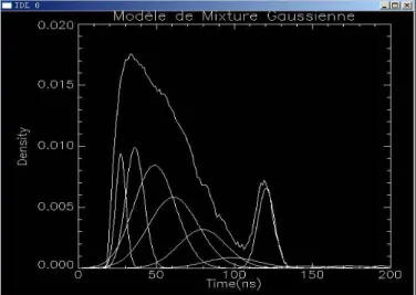
The waveform is interpreted as a mixture of Gaussian curves. The Gaussian represents the water surface, the water column and the seafloor. The Gaussian Mixture Model is applied to the waveform to study the position and the shape of
the bottom peak (Fig. 1). The amplitude and the kurtosis of the bottom peak are a function of the bottom material, the presence and density of seaweed and the quality of the water column. Our approach used the Expectation-Maximization (EM) algorithm which is widely used to unmix a Gaussian mixture distribution. The EM algorithm needs, as an initial parameter, the number of populations that compose the mixture. As this number is not known, the algorithm tries with an increasing number of populations (5 to 10). For each attempt, the Gaussian mean that is the closest to the depth is retrieved and defined as the bottom peak signal. Then the bottom peak signal is subtracted from the bottom peak of the waveform. The lowest difference of all the combinations will be the final result. This method is applied over homogeneous seabed areas to study the correlation between the seafloor sediment type and the Gaussian parameters. The parameters used are the standard deviation (SIG) and density (P) (i.e. contribution, in percent, of each Gaussian in the distribution).
F. Roughness
This parameter is a first approach for bottom classification. It is based only on elevation data. The roughness is obtained by rasterizing the elevation point cloud. The roughness is the standard deviation of elevation for all the points that lie within a pixel. The raster resolution (1 pixel = 10 m x 10 m square) gives an average of 8 laser shots per pixel. Indurated sediment (e.g. bedrock, large pebbles, blocks) gives strong roughness (R) values whereas soft sediment (e.g. coarse to fine sand) returns lower values.
G. Slope Angle and Direction
The X, Y, and Z values of the Lidar points within each pixel are input into a multiple linear regression algorithm, which in Interactive Data Language (IDL) is called REGRESS. The output of this algorithm is two values, the slope in the X direction and the slope in the Y direction (i.e. the gradient). The overall slope is the pythagorean sum of these two values, which is then converted to degrees. The aspect is calculated as the inverse tangent of the two values and converted to degrees.
Figure 1. Example of the Gaussian Mixture Model applied to waveforms of the shallow blue-green channel. Here a set of 10 populations is attempted. The 7th population correspond to the bottom peak.
Roughness and slope parameters were calculated using LiDAR Tools with ENVI, a free Open-Source package available on internet. The author of this package is David Streutker from Boise Center Aerospace Lab of the Idaho State University.
III. RESULTS AND DISCUSSION
A. Moment Method
The first area had STD=0.86 ns indicating a moderately sorted bottom material of fine to medium sand with a kurtosis of K=0.14. In the second area, the value of STD=1.12 ns indicated a poorly sorted bottom with K=1.03. The third area had STD=0.76 ns indicating a moderately sorted bottom of medium to fine sand.
In the cumulative frequency curve, the weight of the water column increased with the depth (18.3% at 3.8 m, 22.6% at 5.0 m, 34.6% at 8.1 m). In contrast, the bottom percentage decreased with depth as a result of the water column attenuation effect (26.9% at 3.8 m, 12.9% and 5.0 m, 10.8% at 8.1 m). The weight also reflects specific bottom signature such as the presence of seaweed. In the first area, two populations are represented at 26.9% and 13.4%. Reflecting the density of seaweed growth, the second percentage represents the proportion of the laser signal that penetrates the vegetation and reaches the real bottom. In the second area, three significant populations exist: 12.9%, 15.7% and 9.8%. This is due to the existence of two seaweed populations of different heights. The real bottom hit is represented by the last percentage value.
The third area presents only one significant bottom percentage at 10.8%, indicating a seabed sediment facies with no seaweed. A similar approach has been developed over a sand dune field to calculate the variation of the density along the dune profile.
B. Gaussian Mixture Model
Three subsets of the first area have been defined. These correspond to different mixture of sand and pebble. One sub-area has small sand dunes. The first sub-sub-area composed of very-fine to fine sand has a SIG of 5.20 with P of 0.08. The second sub-area, composed of coarse sand, has a SIG of 7.22 with a P at 0.33. The third sub-area, is composed with fine sand and has a small sand dune field. Its SIG is 8.49 with a P of 0.58. This approach shows that each sediment type has a specific SIG. The P value sheds light on some bottom type and sediment processes. Over the fine sandy area, where the water current creates turbidity, the P value of the bottom represents only 0.08% of the whole signal, revealing a masking by the turbid plume. With coarser sand, the P value represents about a third of the signal, reflecting a relatively clear water column (less turbidity due to larger grain size) and also a flat seafloor. Where sand dunes exist, P is higher at 0.58. This reflects the multiple returns due to the bottom morphology.
The second area has a SIG of 6.76 with a P of 0.16. The results are quite comparable in the third area with a SIG of 6.88 and a P of 0.26. It might be difficult to classify the bottom type here if only the SIG values were available, but the P value is a good indicator of seaweed. The low P value over the second area is the result of masking by dense Laminaria field that is present in the area. The seaweed masks the real bottom. The third area is mainly composed of fine to medium sand, a grain size that under certain hydrodynamic conditions can produce turbid water. In the present study, a severe thunderstorm the day before the survey produced heavy turbidity in the area.
More work is needed to follow up on the Gaussian Mixture Model, to overcome certain limitations. All the Gaussians are symmetric around their mean values. Therefore a skewness coefficient is not available. Or the waveform’s bottom peaks are not symmetric and a skewness coefficient can be estimated.
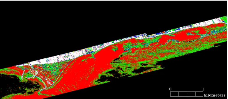
Figure 2. A raster representing the seabed roughness over the Paspébiac shoreface area. Areas in red are mainly composed of fine to medium sand without seaweed. Areas in green represent a mix of mainly coarse to fine sand with some medium to large pebbles, few bedrock outcrops and little seaweed growth. The blue-white area is a mix of coarse sand with small to medium pebbles and some exposed bedrock with dense seaweed growth.
To estimate this coefficient, a theoretical approach is needed. With the waveform’s bottom peak and the results of the Gaussian Model, a theoretical bottom peak can be produced by taking the left half of the fitted Gaussian and adding the left part of the waveform bottom peak. This new bottom peak is then fitted with two distribution models, the Maxwell-Boltzman and the Rayleigh distributions.
C. Roughness
This parameter is strongly dependant of the local bottom slope. To avoid bias in the result, the roughness is calculated only where the slope is 5° or less. The roughness calculated for the three zones in this study is, respectively, 0.11, 0.23 and 0.05. The results (Fig 2) show that poorly sorted coarse sediment and bedrock outcrop exhibit the highest roughness values (R=0.23). The Laminaria field has a relatively high roughness (R=0.11). The sandy area has the lowest roughness values (R=0.05).
D. Slope angle and direction
The mean slope over the survey area is very low - 3.3°. The lowest slope, almost horizontal, is found in the sandy area. The maximum slope (31°) is in the bedrock area. The sandy area has a mean slope of 1.0° toward an azimuth 165°. The mixed area has a slope of 2.1° and a mean orientation of 191°. The bedrock area has the highest mean slope values with 4.8° and a mean orientation of 160°.
Slope is a good indicator of seafloor type since each type of material has a different mean value. The orientation of the structures gives valuable information on the sedimentary processes and waves energy environment. Over the sandy area, there are two mean orientations, 165° and 203°, values that represent two different sets of sand dunes. The slope of 165° relates to sand dunes that are oriented NNW-SSE. These are the expression of the westward-oriented long shore current in the area. At greater depth, there is a different mean slope of 203°. Those sand dunes fields are oriented SSW-NNE and are the results of the storms that comes from the Gulf of St-Lawrence.
IV. SUMMARY AND CONCLUSION
This preliminary report shows that the SHOALS-3000 is able to “see” the bottom and provide information on its geology.
The moment method shows that the SHOALS-3000 waveforms are responsive to the sea-floor sediment and classification, including the presence or absence of seaweed. The correlation of the reflectance with the depth and bottom material shows that the water column effect is weak relative to the bottom material reflectance. Also the density of the seaweed growth is expressed by the reflectance value (higher seaweed density = lower reflectance value).
The Gaussian Mixture Model produced useful results in regard to the fit of the bottom peak signal. We are currently computing a Gaussian mixture raster. This approach shows that each sediment type has a specific Gaussian parameter. The density value of the Gaussian reflects some bottom type and
sediment processes. However, even with the promising results obtained with this method, there is a need for some further development to obtain a better fit of the waveform bottom peak.
The roughness parameter gives a very good first-order classification of the seafloor. Combined with slope information, this can be very useful for interpretation of the seafloor material and processes.
All of these methods need to be merged and integrated to a neural network to develop a more efficient tool for bottom classification and sedimentary process monitoring.
ACKNOWLEDGMENT
The authors thanks the Canadian Network of Centres of Excellence GEOIDE for financial support, Natural Resources Canada and Fisheries and Oceans Canada for material support in the field, Optech, Lasermap, Image Plus, Inc and Dynamic Aviation for their constant support and presence during the preparation of the mission and during the survey, and all the students from several universities without whom the field work would never have been done. A. Cottin personally thanks Dikanaina Harrivel and Ohad Gal for their support on the Gaussian Mixture Model and David Streutker for his outstanding open-source tool LiDAR Tools (http://geology.isu.edu/BCAL/tools/EnviTools) for ENVI.