Analyse multifractale utilisant le taux de précipitations dans cas de typhon en 2012, Corée

(1)

HAL Id: tel-03136520

https://pastel.archives-ouvertes.fr/tel-03136520

Submitted on 9 Feb 2021

HAL is a multi-disciplinary open access

archive for the deposit and dissemination of sci-entific research documents, whether they are pub-lished or not. The documents may come from teaching and research institutions in France or abroad, or from public or private research centers.

L’archive ouverte pluridisciplinaire HAL, est destinée au dépôt et à la diffusion de documents scientifiques de niveau recherche, publiés ou non, émanant des établissements d’enseignement et de recherche français ou étrangers, des laboratoires publics ou privés.

Analyse multifractale utilisant le taux de précipitations

dans cas de typhon en 2012, Corée

Jisun Lee

To cite this version:

Jisun Lee. Analyse multifractale utilisant le taux de précipitations dans cas de typhon en 2012, Corée. Ingénierie de l’environnement. Université Paris-Est; Institute of Fisheries Science (Corée (République)), 2020. Français. �NNT : 2020PESC1007�. �tel-03136520�

(2)

Thése présentée pour obtenir le grade de Docteur de l'Université Paris-Est

Spécialité: Sciences et Techniques de Meteorologie et l'Environnement par

Jisun Lee

Ecole Doctorale : Sciences, Ingénierie et Environnement

Multifractal Analysis on the Rainfall Rate

in Typhoon Cases in 2012, Korea

Thése soutenue le 15 Janvier 2020 devant le jury composé de :

Klaus Fraedrich Rapporteur

Cheol-Hwan You Rapporteur

Mi-Young Kang _Examinateur

Auguste Gires Examinateur

Kyung-Sik Kim _Examinateur

Ioulia Tchiguirinskaia co-superviseur

Dong-In Lee Directeur de thése

(3)

i

Analyse multifractale utilisant le taux de précipitations

dans cas de typhon en 2012, Corée

Jisun Lee

HM&Co, É cole des ponts, Sciences, Ingénierie et Environnement, É cole doctoral, Université Paris-Est

Department of Environmental Atmospheric Science, The Graduate School, Pukyong National University

Résumé

L'approche multifractale a été utilisée pour analyser le taux de précipitations de trois typhons (Khanun, Bolaven et Sanba) qui ont frappé la Corée du Sud en passant par l'île de Jeju vers la péninsule coréenne en 2012. Les données sur le taux de précipitations sont obtenues à partir d'un radar en bande S exploité par la Corée Administration météorologique (KMA) et la simulation de modèle CReSS.

L'analyse multifractale a été réalisée à l'aide de l'analyse Trace Moment (Schertzer et Lovejoy, 1987) et de l'analyse Double Trace Moment (Lavallée et al., 1992) pour quantifier l'intermittence moyenne à l'aide de sa co-dimension fractale C1 et de sa multifractalité. index 𝛼, qui mesure la rapidité avec laquelle évolue l'intermittence pour l'ordre statistique supérieur avec une grande quantité de données spatio-temporelles.

Premièrement, avec les données radar, l’analyse spectrale a été réalisée pour vérifier la prudence du champ. Dans le cas des typhons Khanun, Bolaven et Sanba, les valeurs moyennes de l’exposant d’échelle β pour l’analyse spectrale sont respectivement de 1,92 (Khanun), 1,710 (Bolaven) et 2,233 (Sanba), toutes

(4)

ii

hauteurs des domaines de 256 km. × 256 km. Alors que 2.515 (Khanun), 2.553 (Bolaven) et 2.513 (Sanba) dans la taille du domaine 64 km × 64 km. Tous les champs de différentes tailles de domaines à différentes altitudes étaient conservateurs.

En analyse TM et DTM, avec l'ordre des moments q et (q, η), il est montré que K (q) et K (q, η) satisfont à la forme universelle présentant les paramètres de messagerie unifiée 𝛼 et C_1. Chaque paramètre indique le degré de multifractalité du processus (α) et la codimension de la singularité moyenne du champ (C_1). Dans tous les cas, les champs pluviométriques étaient constants en basse altitude (1, 2 km), alors que les fluctuations étaient plus marquées en haute altitude.

Pour vérifier le résultat de l'observation radar, nous avons également utilisé le taux de précipitation obtenu par simulation du modèle CReSS. En conséquence des paramètres de messagerie unifiée de tous les cas du modèle CReSS, uniquement dans le cas de Khanun, α est inférieur à 1 dans les deux domaines. D'autre part, α est supérieur à 1 avec Bolaven et Sanba dans les deux domaines.

Avec le résultat, il est montré qu'il existe une dépendance de 𝛼 avec l'altitude qui montre la déduction de la configuration du champ de précipitations dans chaque altitude avec les paramètres UM. Cela permet de voir l'évolution du champ de précipitations. Lorsque le typhon a traversé l’île de Jeju, où se trouve le mont Halla, il a commencé à diminuer les cyclones, libérant ainsi son humidité sous forme de pluie torrentielle sur l’île. Étant donné que le stade de tous les typhons était en phase d'affaiblissement ou de dissipation, les paramètres UM montrent que le cisaillement du vent a incliné le vortex pour obtenir les différentes configurations des champs de précipitations à chaque altitude.

(5)

iii

Multifractal Analysis on the Rainfall Rate

in Three Typhoon Cases, Korea

Jisun Lee

HM&Co, É cole des ponts, Sciences, Ingénierie et Environnement, É cole doctoral, Université Paris-Est

Department of Environmental Atmospheric Science, The Graduate School, Pukyong National University

Abstract

The multifractal approach was used to analyze the rainfall rate of three typhoons (Khanun, Bolaven, Sanba) that struck South Korea passing through Jeju Island to the Korean peninsula in 2012. The rainfall rate data are obtained from S-band radar operated by the Korea Meteorological Administration (KMA) and the model simulation CReSS.

The multifractal analysis was performed with the help of Trace Moment analysis (Schertzer and Lovejoy, 1987) and Double Trace Moment analysis (Lavallée et al., 1992) to quantify the mean intermittency with the help of its fractal co-dimension 𝐶₁ and its multifractality index 𝛼, which measures how fast the intermittency evolves for the higher order of statistics with a large amount of space-time data.

Firstly, with the radar data, the spectral analysis was done to check the conservativeness of the field. In the case of Typhoon Khanun, Bolaven, and Sanba, the average values of scaling exponent 𝛽 for spectral analysis are, respectively, 1.92 (Khanun), 1.710 (Bolaven), and 2.233 (Sanba) in all heights of the domain sizes 256 km × 256 km. While 2.515 (Khanun), 2.553 (Bolaven),

(6)

iv

and 2.513 (Sanba) in the domain size 64 km ×64 km. All the fields of different sizes of domains at different altitudes were conservative.

In TM and DTM analysis, along with the moment order q, and (q,η), it is shown that K(q) and K(q,η) satisfies the universal form presenting the UM parameters 𝛼 and 𝐶1. Each parameter shows the degree of multifractality of the

process (α) and the codimension of the mean singularity of the field (𝐶₁). In all the cases, the rainfall fields were constant in low altitudes (1, 2 km) while it shows more fluctuation in higher altitudes.

To compare the result of the radar observation, the rainfall rate obtained by CReSS model simulation was also used. As a result of the UM parameters of all cases from CReSS model, only with the Khanun case, α is less than 1 in both domains. On the other hand, α is larger than 1 with Bolaven and Sanba in both domains.

With the result, it is shown that there is a dependence of 𝛼 along with the altitude which shows the deduction of the pattern of the rainfall field in each altitude with the UM parameters. This enables to see the development of the rainfall field. As the typhoon passes through the Jeju Island, where there is Halla Mountain, it started to diminishing cyclones unleashing their moisture as torrential rainfall on the island. Since the stage of all the typhoons was in weakening or dissipating stage, the UM parameters show that the wind shear tilted the vortex to have the different patterns of the rainfall fields in each altitude.

(7)

v

5.1. Typhoon Khanun ………..……… 31 5.1.1. Environmental description …..……… 31 5.1.2. Observational results ………. 35 5.1.3. Multifractal analysis ………. 44 5.2. Typhoon Bolaven ………. 69 5.2.1. Environmental description ………. 69 5.2.2. Observational results ……… 73 5.2.3. Multifractal analysis ……… 82 5.3. Typhoon Sanba ……….. 110 5.3.1. Environmental description ………. 110 5.3.2. Observational results ……….……… 114 5.3.3. Multifractal analysis ……… 123

6. Summary and Conclusion 151 References ………...……….. 155

(10)

viii

List of Tables

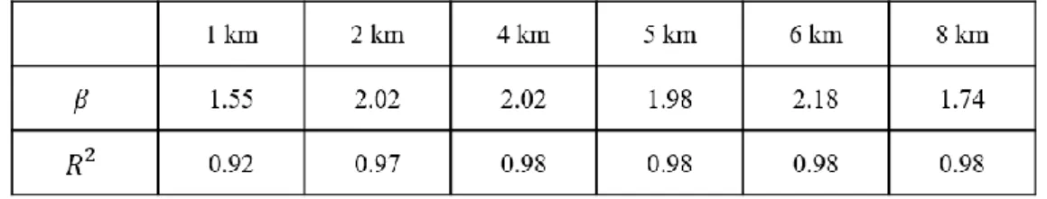
Table 5.1.1.

The values of 𝜷 and 𝑹𝟐_{after spectral analysis}

in the domain size 256 km × 256 km with the case

of Typhoon Khanun. 45

Table 5.1.2. The estimated UM parameters from TM and

DTM in the domain size 256 km × 256 km. 52 Table 5.1.3.

The values of 𝜷 and 𝑹𝟐_{after spectral analysis}

in the domain size 64 km × 64 km with the case

of Typhoon Khanun. 54

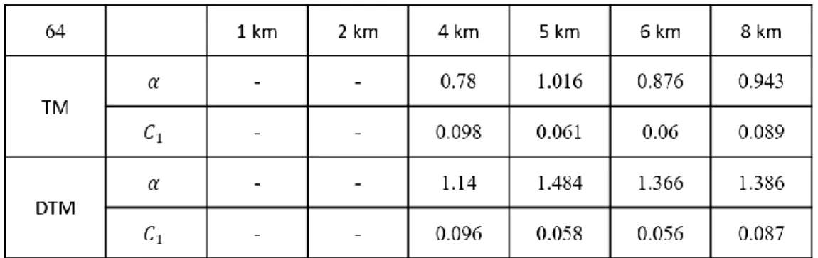
Table 5.1.4.

The estimated UM parameters from TM and

DTM in the domain size 64 km × 64 km. 58

Table 5.1.5.

The estimated UM parameters from TM and DTM analysis with the dataset of CReSS in the

domain 256 km × 256 km and 64 km × 64 km. 65 Table 5.2.1.

The same as Table 5.1.1 but with Typhoon

Bolaven. 83

Table 5.2.2.

Bolaven. 90

Table 5.2.3.

Bolaven. 92

Table 5.2.4.

Bolaven. 99

Table 5.2.5.

Bolaven. 106

Table 5.3.1. The same as Table 5.1.1 but with Typhoon Sanba. 124 Table 5.3.2. The same as Table 5.1.2 but with Typhoon Sanba. 131 Table 5.3.3. The same as Table 5.1.3 but with Typhoon Sanba. 133 Table 5.3.4. The same as Table 5.1.4 but with Typhoon Sanba. 140 Table 5.3.5. The same as Table 5.1.5 but with Typhoon Sanba. 147

(11)

ix

List of Figures

Fig. 2.1.

The map of the selected area for this study indicated with the red box and the radar observation sites shown with the red dots (Gosan and Seongsanpo) in Jeju Island, Korea.

6

Fig. 2.2.

The schematic diagram of microphysical process

used in the model calculation. 7

Fig. 3.1.

The map of the selected domain when using the

numerical model CReSS. 14

Fig. 4.1.

The schematic diagram of the rainfall intensity on

the selected domain of typhoon. 16

Fig. 4.2.

The fractal dimension calculated at 1940 LST 18 July 2012 with (a) radar at 5 km with the domain size 265 km × 265 km, (c) in the domain size 64 km × 64 km with the threshold 1 mm/hr (black), 3 mm/hr (blue) and 5 mm/hr (red). (b) and (d) indicates the area with the rainfall field with the black shaded area along with the different thresholds.

19

(12)

x

Fig. 4.3.

The fractal dimension calculated at 2330 LST 27 August 2012. (a) radar at 5 km with the domain size of 265×265 with the threshold 1 mm/hr (black), 5 mm/hr (blue) and 10 mm/hr (red), (c) in the domain size of 64 km × 64 km with the threshold 1 mm/hr (black), 3 mm/hr (blue) and 5 mm/hr (red). (b) and (d) indicates the area with the rainfall field with the black shaded area along with the different thresholds.

20

Fig. 4.4.

The fractal dimension calculated at 1940 LST 18 September 2012 with (a) radar at 5 km with the domain size 265 km × 265 km, (c) in the domain size 64 km × 64 km with the threshold 1 mm/hr (black), 3 mm/hr (blue) and 5 mm/hr (red). (b) and (d) indicates the area with the rainfall field with the black shaded area along with the different thresholds.

21

Fig. 4.5.

Diagram of cascade phenomenon for (a) 1-dimension and (b) 2-1-dimension.

23

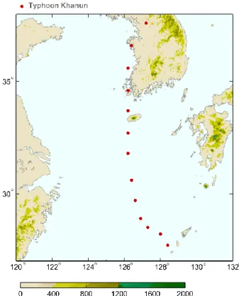
Fig. 5.1.1.

The track of typhoon Khanun. The red dots

indicate the location of the typhoon center. 32

Fig. 5.1.2.

The daily accumulated rainfall on 18 July 2012 in Korea.

32

Fig. 5.1.3.

The graph of typhoon center pressure (hPa) in red

(13)

xi

Fig. 5.1.4.

The synoptic flow at 1200 UTC on 18 July 2012. (a) at the surface showing the pressure (sea level pressure, hPa), (b) at 850 hPa showing the equivalent potential temperature (K), (c) at 500 hPa showing the relative vorticity (10−5_𝑠−1_{), and}

(d) at 300 hPa showing the geopotential height (m) with wind vector.

34

Fig. 5.1.5.

The wind field superimposed on the radar reflectivity (dBZ) on each altitude (1, 2, 4, 5, 6, 8 km) at 1730 LST, 1930 LST, 2030 LST and 2130 LST during Typhoon Khanun.

36

Fig. 5.1.6.

The vertical wind field superimposed on the radar reflectivity (dBZ) on each time step. Vertical cross section is indicated with the red line (A-B).

39

Fig. 5.1.7.

The horizontal distribution of wind field of divergence (red) and convergence (blue) with the radar reflectivity (contour).

41

Fig. 5.1.8.

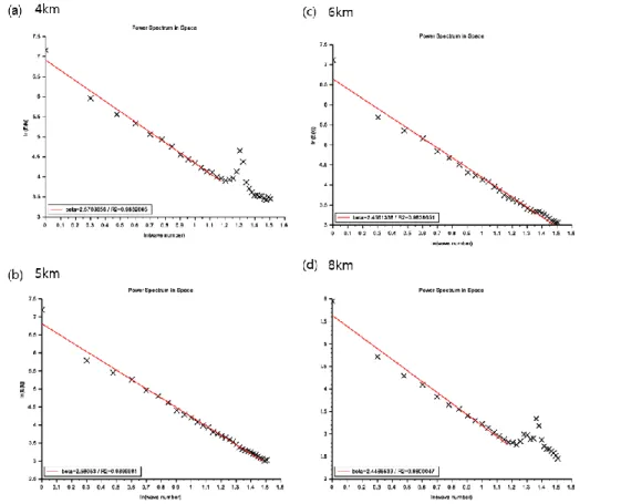
The result of spectral analysis, ln 𝐸(𝑘) as a function of ln 𝑘 with the rainfall rate retrieved from radar data on every height (a) 1 km, (b) 2 km, (c) 4 km, (d) 5 km, (e) 6 km and (f) 8 km in 256 km × 256 km size of the domain.

45

(14)

xii

The result of TM analysis obtained from the radar dataset in the 256 km × 256 km sizes of the domain. The scaling behavior with the value of different q from 0.1 to 7.0 at 1 km, 2 km, 4 km, 5 km, 6 km and 8 km (a, b, c, d, e, f). 𝐾(𝑞) (black) is obtained in the graph (g, h, i, j, k, l) and the multifractal parameters retrieved from TM analysis are shown on the left top corner.

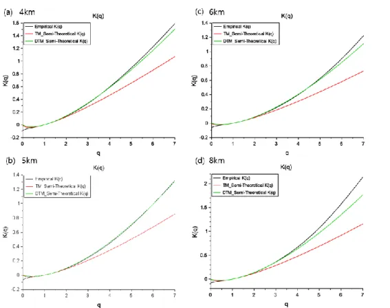
Fig. 5.1.10.

The scaling moment function 𝐾(𝑞) obtained from the empirical dataset (black), from using UM parameters obtained from TM (red), from using UM parameters obtained from DTM (green).

49

Fig. 5.1.11.

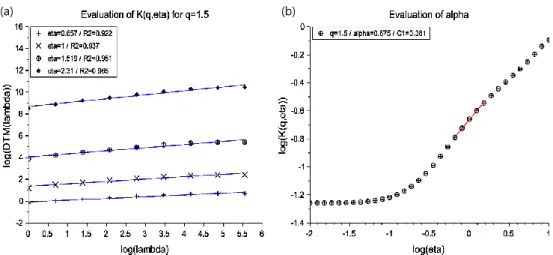
The result of DTM analysis obtained from the radar dataset in the 256 km × 256 km sizes of the domain. The scaling behavior with the value of different 𝜂 from 0.1 to 2.5 at 1 km, 2 km, 4 km, 5 km, 6 km and 8 km (a, b, c, d, e, f) at fixed 𝑞 = 1.5. DTM curve is shown in (g, h, I, j, k, l).

50

Fig. 5.1.12.

The UM parameters obtained from TM and DTM.

52

Fig. 5.1.13.

The same as Fig. 5.1.8 but in the altitudes of (a) 4 km, (b) 5 km, (c) 6 km, and (d) 8 km in the

domain size 64 km × 64 km. 53

Fig. 5.1.14.

The same as Fig. 5.1.9 but in the altitudes of (a,e)

(15)

xiii

4 km, (b,f) 5 km, (c,g) 6 km, and (d,h) 8 km in the domain size 64 km × 64 km.

Fig. 5.1.15.

The same as Fig. 5.1.10 but in the altitudes of (a) 4 km, (b) 5 km, (c) 6 km, and (d) 8 km in the domain size 64 km × 64 km.

56

Fig. 5.1.16.

The same as Fig. 5.1.11 but in the altitudes of (a,e) 4 km, (b,f) 5 km, (c,g) 6 km, and (d,h) 8 km in the domain size 64 km × 64 km.

57

Fig. 5.1.17.

The same as Fig. 5.1.12 but in domain 64 km ×

64 km. 58

Fig. 5.1.18.

The accumulated rainfall field on each altitudes

of typhoon Khanun. 59

Fig. 5.1.19.

The result of spectral analysis from CReSS model

dataset. 60

Fig. 5.1.20.

The result of TM analysis obtained from CReSS model dataset in domain 256 km × 256 km. (a)

(16)

xiv

The scaling behavior with the value of different q from 0.1 to 7.0 and (b) the graph of K(q) with the values of multifractal parameters indicated which were obtained from TM analysis. (c) The scaling moment function K(q) obtained from the empirical dataset (black), from using UM parameters obtained from TM (red), from using UM parameters obtained from DTM (green).

Fig. 5.1.21.

The result of DTM analysis with CReSS model dataset in domain 256 km × 256 km. (a) The scaling behavior with the value of different 𝜼 from 0.1 to 2.5 at fixed q=1.5. (b) DTM curve with multifractal parameters.

62

Fig. 5.1.22.

The same as Fig. 5.1.19 but in the domain 64 km

× 64 km. 63

Fig. 5.1.23.

The same as Fig. 5.1.20 but in the domain 64 km

× 64 km. 64

Fig. 5.1.24.

64 km. 65

Fig. 5.1.25.

Comparison between the empirical K(q) for each height of the radar data and the CReSS model in the domain size of 256 km × 256 km of typhoon Khanun. The blue dots correspond to the K(q)

(17)

xv

values for each q value; the black lines are the linear regression fits.

Fig. 5.1.26.

The same as Fig. 5.1.25 but with the domain 64

km × 64 km. 68

Fig. 5.2.1.

The track of Typhoon Bolaven. The red dots indicate the location of the typhoon center.

70

Fig. 5.2.2.

The daily accumulated rainfall on 27 August 2012

in Korea. 70

Fig. 5.2.3.

and the maximum wind speed (m/s) in blue. 71

Fig. 5.2.4.

The synoptic flow at 1200 UTC on 27 August 2012. (a) at the surface showing the pressure (sea level pressure, hPa), (b) at 850 hPa showing the equivalent potential temperature (K), (c) at 500 hPa showing the relative vorticity (10−5_𝑠−1_{), and}

(d) at 300 hPa showing the geopotential height (m) with wind vector.

72

Fig. 5.2.5.

The same as Fig. 5.1.5 but with Bolaven case. 74

(18)

xvi

The same as Fig. 5.1.6 but with Bolaven case.

Fig. 5.2.7.

The same as Fig. 5.1.7 but with case of typhoon

Bolaven. 79

Fig. 5.2.8. _{The same as Fig. 5.1.8 but with Bolaven case.} 83

Fig. 5.2.12.

The UM parameters obtained from TM and DTM. 90

Fig. 5.2.13.

The same as Fig. 5.2.8 but in the domain size 64

km × 64 km. 92

Fig. 5.2.14.

km × 64 km. 94

Fig. 5.2.15.

km × 64 km. 96

Fig. 5.2.16.

(19)

xvii

km × 64 km.

Fig. 5.2.17.

64 km. 99

Fig. 5.2.18.

The same as Fig. 5.1.18 but with the case of

typhoon Bolaven. 100

Fig. 5.2.19.

The result of spectral analysis from CReSS model

dataset with domain 256 km × 256 km. 101

Fig. 5.2.20.

Fig. 5.2.21.

Fig. 5.2.22.

The result of spectral analysis by CReSS model

dataset in domain 64 km × 64 km. 104

Fig. 5.2.23.

(20)

xviii

64 km.

Fig. 5.2.24.

64 km. 106

Fig. 5.2.25.

The same as Fig. 5.1.25 but with the case of

Typhoon Bolaven. 108

Fig. 5.2.26.

The same as Fig. 5.2.25 but in the domain size of

64 km × 64 km. 109

Fig. 5.3.1.

The track of Typhoon Sanba. The red dots

indicate the location of the typhoon center. 111

Fig. 5.3.2.

The daily accumulated rainfall on 17 September

2012 in Korea. 111

Fig. 5.3.3.

and the maximum wind speed (m/s) in blue. 112

Fig. 5.3.4.

The synoptic flow at 1800 UTC on 16 September 2012. (a) at the surface showing the pressure (sea

(21)

xix

level pressure, hPa) and wind vector, (b) at 850 hPa showing the equivalent potential temperature (K) and wind vector, (c) at 500 hPa showing the relative vorticity (10−5_𝑠−1_{) and wind vector, and}

(d) at 300 hPa showing the geopotential height (m) and wind vector.

Fig. 5.3.5.

The same as Fig. 5.1.5 but with Typhoon Sanba

case. 115

Fig. 5.3.6.

The same as Fig. 5.1.6 but with Sanba case. 118

Fig. 5.3.7. _{The same as Fig. 5.1.7 but with typhoon Sanba.} 120

Fig. 5.3.8.

Fig. 5.3.9.

Fig. 5.3.10.

Fig. 5.3.11.

(22)

xx

Fig. 5.3.12.

The UM parameters obtained from TM and DTM. 131

Fig. 5.3.13.

km × 64 km. 133

Fig. 5.3.14.

km × 64 km. 135

Fig. 5.3.15.

km × 64 km. 137

Fig. 5.3.16.

km × 64 km. 138

Fig. 5.3.17.

64 km. 140

Fig. 5.3.18.

The same as Fig. 5.1.18 but with the case of typhoon Sanba.

(23)

xxi

Fig. 5.3.19

The result of spectral analysis by CReSS model

dataset in domain 256 km × 256 km. 142

Fig. 5.3.20.

Fig. 5.3.21.

Fig. 5.3.22.

64 km. 145

Fig. 5.3.23.

64 km. 146

Fig. 5.3.24.

64 km. 147

Fig. 5.3.25.

(24)

xxii

Fig. 5.3.26.

The same as Fig. 5.3.25 but with the domain 64

(25)

1

1. Introduction

The typhoon has become an essential issue as it brings huge damage and its occurrence frequency has been increased since 2001 in Korea. Many analysis related to typhoon cases has been conducted with many different points of view. Park et al. (2006) found out the change of statistical characteristics of typhoons during 50 years (1954-2003) by analyzing the changes in air temperature and sea surface temperature. Kim et al. (2006) found out the increased heavy rainfall associated with typhoons after 1978. By Park and Lee (2007), synoptic features of typhoon Rusa was investigated by performing the numerical model MM5. Lee and Choi (2010) also used the numerical simulation (WRF) to examine the predictability of the torrential rainfall with the typhoon case of Rusa and its detailed mesoscale precipitation distribution. Kim et al. (2010) used WRF model and dropsonde data assimilation to reduce the typhoon track forecast and determine the sensitivities of storm activities during typhoon Sinlaku and Jangmi in 2008. Park et al. (2011) analyzed the characteristics of typhoon activity from 1977 to 2008 and divided it into two decades and revealed that rainfall increased in the later period due to certain factors led intensification of typhoons, such as warmer sea surface temperature and high humid mid-troposphere and weaker vertical wind shear in the domain. Kim et al. (2011) provided better sensitivity guidance for real-time targeted observation operations when using the MM5 model simulation. Kim et al. (2016) built quantitative statistical datasets from rainfall data during typhoon cases from 1966 to 2009 and analyzed the characteristics of typhoon activity (e.g., TC genesis location, TC path, recurving position, and intensity) and related spatio-temporal changes in rainfall. Kim and Moon (2019) estimated rainfall in typhoons approached Korea during 2001 – 2016 and classified in different types of wind, rain, or wind/rain dominant to guide better prediction with satellite estimated rainfall data.

July, August, and September in 2012, three typhoons (Khanun, Bolaven and Sanba) struck South Korea in each month passing through Jeju Island to the Korean peninsula leading to severe damages. Jeju island is located in the southern part of Korea and is where all of the typhoons made the first landfall. On this island, there are two S-band Doppler radars on the east and west coast operated by Korea Meteorological Administration (KMA) which is useful to obtain the data for radar analysis.

(26)

2

In the past years, many case studies of typhoons were carried out to analyze the phenomenon with the help of two radars on Jeju island. Recently, Yoo and Ku (2017) used radar and rain gauge data to see the orographic effect on the rainfall rate field during typhoon Nakri in 2014. Lee et al. (2018) studied the microphysical process with the orographic effect by analyzing dual Doppler analysis with the radar and numerical model CReSS during typhoon Khanun. Kim et al. (2018) obtained echo motion vectors from the radar to use Variational Echo Tracking (VET) method for nowcasting of precipitation system including six typhoon cases during 2011-2013.

However, there is a lack of studies investigating the linearity of the typhoon especially by using radar data. To see the detailed linearity of the typhoon, the multifractal framework was applied in this study by using the rainfall rate dataset obtained from the radar.

The multifractal framework is known as one of the convenient methods to analyze the variable fields over a wide range of space-time scales in geophysical fields such as rainfall. With the development of multifractals framework, it became possible to define stochastic processes modeling rainfall with the help of the physically meaningful parameters. These parameters characterize how the cascade process concentrates the “activity” of a field (e.g., the precipitation rate above a given threshold) at smaller and smaller scales on smaller and smaller fractions of the space. These sets are some small that their dimension is only fractal, not that of the embedding space, and it is smaller and smaller for higher and higher levels of activity (e.g., Parisi and Frisch (1985), Schertzer and Lovejoy (1987)).

There are various examples of case studies of precipitations such as applying a multifractal approach relating to the shape of the cloud system and rain areas (Lovejoy, 1982) or applying the multifractal framework relating to the shape of a cloud system to rainfall intensity (Schertzer and Lovejoy, 1984). As the multifractals are likely the cascade process output, they have been developed and applied in many analyses and simulations in geophysical fields revealing extreme variabilities over a wide range of scales. (Schertzer and Lovejoy, 1987; Gupta and Waymire, 1993; Harris et al., 1996; Marsan et al., 1996; De Lima and Grasman, 1999; Deidda, 2000; Biaou, 2004; Macor et al., 2007; De Montera et al., 2009; Tchiguirinskaia et al., 2011; Gires et al., 2013; Hoang et al., 2014). Also, the extreme rainfall events were investigated by using multifractal analysis in Hubert et al. (1993), Schertzer et al. (2007), and Schertzer et al. (2010). It also covered explaining the climate by Royer et al. (2008) and Lovejoy and Schertzer (2013). The fractal theory expanded the use

(27)

3

for prediction in Marsan et al. (1996), Schertzer and Lovejoy (2004) and Macor et al. (2007).

Despite the benefits of the multifractal framework, there had not been many studies of typhoons since Chygyrynskaia et al. (1995) and Lazarev et al. (1995) on 1D multifractal analysis of the wind field. In Korea, there are only a few studies conducted with the multifractal approach in the meteorological aspect in typhoon cases. Kim et al. (2008) presented a singularity of rainfall to provide evidence of multifractality in four cities in Korea. They found the chaotic property of the moving speed of typhoons is more robust than that of the other three meteorological factors. However, it was not aimed to analyze the precipitation of the typhoon nor did it use the radar data. Also, it was only focused on finding out the multifractal behavior of the chosen factors obtained from the typhoon information provided by KMA.

Therefore, the first motivation of this study is that not enough research was carried out by the approach of explaining the nonlinearity and nonstationary in the multifractal structure by performing the multifractal analysis of typhoons, especially with using the radar data.

Performing the high-resolution numerical experiment for a typhoon is a generally known way to validate the result of observation (Sun and Lee, 2002; Shin and Lee, 2005; Cho and Lee, 2006; Hong and Lee, 2009; Yu and Lee, 2010; Choi et al., 2011). These modeling studies enabled some significant discrepancies between the simulation and observation in both the location and amount of heavy rainfall. In this study, the validation was performed with the numerical model called Cloud Resolving Storm Simulator (CReSS) simulation which provides the high-resolution simulations of high-impact weather systems that are often used for typhoon case studies. Wang et al. (2013) proved that the high-resolution performance of CReSS gave better prediction with the heavy rainfall during the typhoon Morakot. Wang (2015) mentioned that the CReSS model performs the best in the prediction of extreme rainfall events. Also, Chen et al. (2017) used the model to find out the reason of prolonged duration time of the heavy rainfall occurred in Taiwan and Tsujino et al. (2017) revealed that the structure of the outer eyewall plays important roles in the maintenance of long-lived concentric eyewalls by using the CReSS model. The simulation performed for these studies also relatively well capture the location and intensity of the maximum rainfall.

The second motivation of this study is to understand the better dynamics and rainfall by multifractal spatial-temporal analysis with the help of the

(28)

4

measurements of the typhoons by comparing two S-band Doppler radars and the numerical model simulation (CReSS).

The rest of this study is organized as follows. In chapter 2, the explanation of the dataset that was used in this study. Followed up by the chapter 3, the procedure of preparing the dataset of rainfall rate is presented as well as the procedure and the detailed description of the method of the wind field retrieval analysis to find the three-dimensional structure of typhoons (Khanun, Bolaven, and Sanba) during the landfall in Jeju Island. The analysis methodology is described in chapter 4, and the results of the environmental field during each event, wind field analysis and the multifractal analysis by radar data and by the numerical model CReSS are discussed in chapter 5. Finally, some concluding remarks are drawn in chapter 6.

2. Data

2.1. Typhoon track data

Three typhoons that struck South Korea passed through Jeju Island in 2012. Typhoon Khanun was a typhoon with relatively small among the three

(29)

5

typhoons but bringing 400 mm of rain with the maximum wind speed of 24.7 ms-1_{(55.3 mph), which passed through the southwest side of the}

Korean peninsula after passing Jeju island. Typhoon Bolaven passed Jeju Island when it was in a phase of weakening stage, but it brought more than 250 mm of the rainfall amount in 2 days with the wind gusts measured up to 51.8 ms-1 _{considered as the most powerful storm} _{in nearly a decade.}

Typhoon Sanba was also a strong typhoon with the minimum center pressure reaching 900 hPa and recorded the maximum wind speed of 55.9 ms-1 _{(125 mph) and brought 400 mm of rainfall. After passing Jeju}

Island, it moved to North Korea, passing through the middle of the Korean peninsula.

The location of the typhoon center (the longitude and latitude) is gathered with the maximum wind speed to demonstrate the intensity of each typhoon. It was given information from the national typhoon center in KMA (Korea Meteorological Administration). The general information of typhoon is updated in real-time containing the location and the minimum pressure of typhoon center, the maximum wind speed, the radius of the typhoon, intensity, size, direction, and speed of the movement of the typhoon.

2.2. Automatic weather station (AWS)

An AWS is an automated weather station to measure from remote areas. It will typically contain the data logger and save the data from meteorological sensors. The AWS measures the surface data of the rainfall, temperature, humidity pressure, wind speed, and wind direction. Some stations also have additional instruments, but most of the stations have a thermometer, anemometer, wind vane, hygrometer, and barometer. In Korea, there are 510 sites in total, and the data that were used in this study was obtained from 237 sites, including all the sites (35 sites) in Jeju Island. The locations and the daily accumulated rainfall was obtained to see the accumulated rainfall patterns in each typhoon.

2.3. NCEP/NCAR reanalysis data

NCEP/NCAR reanalysis data was provided from Earth system research laboratory and National Oceanic and Atmospheric Administration (NOAA) Office of Oceanic and Atmospheric Research (OAR) laboratories. The NCEP/NCAR reanalysis data has been used to perform data assimilation since 1948. The data contains global grids of spatial coverage and 4-time daily, daily, and monthly temporal coverage with 17 pressure levels and 28 sigma levels (Kalnay et al., 1996). The dataset of wind u, v, air temperature, geopotential height, relative humidity, potential temperature,

(30)

6

and precipitation was used to construct the weather chart for each case.

2.4. Doppler Radar data

The radar dataset was obtained when the typhoon approached Jeju Island on each case. The primarily selected radar site is Gosan (GSN, 33.29°N, 126.16°E, 103 m asl (above sea level)), Seongsanpo (SSP, 33.38°N, 126.88°E, 18.62 m asl) in Jeju Island operated by KMA covering a radius of 360 km and records the sets of volume distribution of reflectivity and Doppler radial velocity every 10 minutes. The obtained radar data was interpolated into a Cartesian coordinate system with horizontal and vertical grid intervals of 1 km and 0.25 km, respectively. A Cressman-type weighting function was used for the interpolation (Cressman, 1959).

2.5. Cloud Resolving Storm Simulator (CReSS)

Cloud Resolving Storm Simulator (CReSS) is a 3-dimensional non-hydrostatic model developed by the Hydrospheric Atmospheric Research Center (HyARC) of Nagoya University, Japan (Tsuboki and Sakakibara, 2002). It is a three-dimensional, regional, compressible non-hydrostatic model, and this numerical model uses a Cartesian horizontal coordinate system follows a terrain-following coordinate and was projected to with a Lambert conical projection. With this coordinate system, the equations for 3-dimensional momentum, pressure, and potential temperature (θ) are generated which is described in detail by Tsuboki and Sakakibara (2002). Fig. 2.1. The map of the selected area for this study indicated with the red box and the radar observation sites shown with the red dots (Gosan and Seongsanpo) in Jeju Island, Korea.

(31)

7

The equations used in this model include all types of waves, such as Rossby waves, acoustic waves, and gravity waves.

A severe thunderstorm is composed of intense convective clouds. Since convective clouds are highly complicated systems of the cloud dynamics and microphysics, it is required to formulate detailed cloud physical processes as well as the fluid dynamics. Cloud physical processes in CReSS are formulated by a bulk method of cold rain (e.g., Lin et al., 1983; Cotton et al., 1986; Murakami, 1990; Ikawa and Saito, 1991; and Murakami et al., 1994). The bulk parameterization of cold rain considers water vapor, rain, cloud, ice, snow, and graupel (See, Fig. 2.2.).

The initial and lateral boundary conditions were provided by Japan Meteorological Agency Global Spectral model (JMA-GSM) which is a reanalysis data as Grid-Point-Values (GPV) database. It has one of the highest horizontal resolutions of 0.1875 degrees (approximately 20 km) with a time interval of 6 hours. JMA-GSM is more used for deep convection simulation such as typhoon cases since it produces the data up to 10 hPa which contains the information of the lower stratosphere and can detect the effect of significant gravity wave propagation in the upper-level atmosphere. Also, to set the surface fluxes of momentum and energy and surface radiation processes, the sea surface temperature (SST) was used by using one-dimensional, vertical heat diffusion equation (Kondo, 1976; Louis et al., 1981; Segami et al., 1989) are included in the Fig. 2.2. The schematic diagram of microphysical process used in the model calculation.

(32)

8

underground layer for ground temperature prediction. The SST at the initial time is calculated from the dataset of NEAR-GOOS Regional Real-Time Data Base, and it is provided by the Japan Meteorological Agency (JMA). The land use data is used from the dataset of Global Land Cover Characteristics Data Base, which is provided by the U. S. Geological Survey.

The final variables that can be obtained are 3-dimensional wind components (u, v, and w), pressure perturbations (p') and potential temperature perturbations (θ') from the mean state. This is in hydrostatic equilibrium at the starting time of model integration. It can also conduct hydrometeor variables such as mixing ratios of water vapor(𝑞_𝑣), cloud water(𝑞𝑐), rain(𝑞𝑟), cloud ice(𝑞𝑖), snow(𝑞𝑠), and graupel(𝑞𝑔), as well as

the number densities of cloud ice(𝑁𝑖) , snow(𝑁𝑠) , and graupel (𝑁𝑔) .

Moreover, zonal velocity at an altitude of 10 m (us), meridional velocity at an altitude of 10 m (vs), pressure at an altitude of 1.5 m (ps), potential temperature at an altitude of 1.5 m (pts), soil and sea surface temperature (qvs), sensible heat over surface (tgs), latent heat over surface (le), global solar radiation (rgd), net downward short wave radiation (rsd), downward longwave radiation (rld), upward longwave radiation (rlu), cloud cover in lower layer (cdl), middle layer (cdm) and upper layer (cdh), averaged cloud cover (cdave), surface momentum flux for x (usflx) and y (vsflx) components of velocity, surface heat flux (ptsflx), surface moisture flux (qvsflx), cloud waterfall fall rate (pcr), accumulated cloud waterfall (pca), rainfall rate (prr), accumulated rainfall (pra), cloud ice fall rate (pir), accumulated cloud ice fall (pia), snowfall rate (psr), accumulated snowfall (psa), graupel fall rate (pgr), accumulated graupel fall (pga) can be obtained.

The CReSS model has been used to study many aspects of typhoons (Akter and Tsuboki, 2012; Wang et al., 2012; Tsuboki et al., 2015). In this study, only the rainfall rate (prr) was used after all the calculation was conducted.

3. Data Processing

3.1. Radar rainfall rate retrieval

The raw data of radar is in Universal Format (UF) which contains the header (mandatory, optional, data, field) and data (DZ, VR, SW, and CZ). The mandatory header includes the information of radar site, the number of sweeps and rays, altitudes angle and azimuth angle. The optional header or local use

(33)

9

header is not commonly used. The data header includes the type of data and the location of where the data is saved. The field header includes the beam width, Nyquist velocity, the number of the bin, and scale factor. The data includes uncorrected reflectivity, radial velocity, spectrum width, and corrected reflectivity.

In this study, corrected reflectivity was used for rainfall rate retrieval. In order to obtain the rainfall rate, the three Cartesian components of reflectivity were calculated. The rainfall rate was computed in separated heights from the reflectivity of Gosan radar, one of the two radars, by using the Z-R relationship ( Z = a𝑅𝑏_{, radar reflectivity factor 𝑍}

(𝑚𝑚6_𝑚−3₎ , rain rate 𝑅_{(𝑚𝑚 ℎ}−1₎ ) with the values of a=250 and b=1.2, which are the parameters usually used for tropical convective systems.

The retrieved dataset was used for multifractal analysis which was performed on the area of 256 km × 256 km at various altitudes, especially where there was the maximum rainfall amount. Further analysis was performed to cover the limitation of missing data due to the lowest elevation scan angles with the smaller domain with the lower altitudes, the size of 64 km × 64 km.

3.2. Wind field retrieval

Doppler radar is known as a powerful instrument for detecting radial velocity and reflectivity information with high spatial and temporal resolution from the weather system. With the Doppler effect, the Doppler radial wind can be obtained as :

𝑓_𝑑 = −2

𝜆 𝑉𝑟 (3.1)

where 𝑓𝑑 is Doppler shift, 𝑉𝑟 is radial wind and wavelength 𝜆 . In this

case, Positive 𝑉𝑟 means the wind is blowing away from the radar and

negative means the wind is blowing toward the radar. To obtain the wind component from a radial velocity at the observation point, a spherical earth coordinate system (γ, θ, φ) is used with x and y.

However, to gain the three-dimensional wind component, the traditional method of dual-Doppler wind retrieval is presented by Armijo (1969). This

(34)

10

study discovered that combining multiple Doppler radars can obtain a three-dimensional wind structure. This technique only needs one interpolation from a regular Cartesian grid to irregular radar observation points due to the Doppler velocity data interpolated into the Cartesian coordinate system by using a Cressman filter (Cressman, 1959).

𝑟 ∙ 𝑉_𝑟= 𝑢𝑥 + 𝑣𝑦 + (𝑤 + 𝑉_𝑡)𝑧 (3.2)

r which is the distance between the grid point, u, v, and w is the wind component at the specific grid point. 𝑉_𝑡 is the terminal velocity of a raindrop which can be estimated from reflectivity.

To calculate u and v by using two Doppler radar, it is assumed the w=0.

Radar 1 : 𝑟1∙ 𝑉𝑟1 = 𝑢𝑥1+ 𝑣𝑦1+ 𝑤𝑧1 (3.3) Radar 2 : 𝑟2∙ 𝑉𝑟2 = 𝑢𝑥2+ 𝑣𝑦2+ 𝑤𝑧2 (3.4) u =𝑟1𝑦2𝑣𝑟1−𝑟2𝑦1𝑣𝑟2 𝑦2𝑥1−𝑦1𝑥2 (3.5) v =𝑟2𝑦1𝑣𝑟2−𝑟1𝑦2𝑣𝑟1 𝑦2𝑥1−𝑦1𝑥2 (3.6)

By applying u and v to vertical integration of the continuity equation, w can be obtained. ∫_𝐻𝐻2𝜕𝑤_𝜕𝑧 1 𝑑𝑧 = − ∫ ( 𝜕𝑢 𝜕𝑥 + 𝜕𝑣 𝜕𝑦) 𝑑𝑧 𝐻2 𝐻1 (3.7)

(35)

11

the ground that we can assume w = 0. Then vertical integration can be done upward to get w at any certain height. Or it can be assumed that it is much higher than the echo top and vertical integration can be done downward. Once w is obtained, it forms an iteration loop to obtain the wind components in the selected domain.

However, this traditional method has limitations that it needs over-lapped data coverage and the wind along the radar baseline between two radars cannot be obtained. Also, the error can be accumulated due to inaccurate top and bottom boundary conditions for w.

To supplement these limitations, a variational method was developed by Gao et al. (1999, 2004). This method estimates the 3-dimensional wind field by using radial velocity and it prevents the accumulation of errors in the vertical velocity. This method minimizes the sum of squared errors which is indicated a cost function (J), due to discrepancies between observations and analyses and additional constraint terms such as the cost functions 𝐽_𝑂, 𝐽_𝐵, 𝐽_𝐷, and 𝐽_𝑆. The iteration loop of calculation is performed until 𝛿𝐽 = 0.

𝐽 = ∭ ∑𝑚 (𝑐𝑜𝑠𝑡 𝑓𝑢𝑛𝑐𝑡𝑖𝑜𝑛𝑠)2

𝑛=1 𝑑𝑥𝑑𝑦𝑑𝑧 (3.8)

Each cost function that was used in this study is defined as follows:

𝐽 = 𝐽𝑂+ 𝐽𝐵+ 𝐽𝐷 + 𝐽𝑆 (3.9) 𝐽𝑂 = 1 2∑ 𝜆𝑚(𝑉𝑟 𝑚_−𝑉 𝑟𝑜𝑏𝑚)2 𝑚 (3.10) 𝐽_𝐵= 1 2[∑ 𝜆𝑢𝑏(𝑢 − 𝑢𝑏) 2 𝑖,𝑗,𝑘 + ∑𝑖,𝑗,𝑘𝜆𝑣𝑏(𝑣 − 𝑣𝑏)2+ ∑𝑖,𝑗,𝑘𝜆𝑤𝑏(𝑤 − 𝑤𝑏)2] (3.11) 𝐽_𝐷 =1 2∑𝑖,𝑗,𝑘𝜆𝐷𝐷 2 _(3.12)

(36)

12

𝐽_𝑆 =1

2[∑ 𝜆𝑢𝑠(∇ 2_𝑢)2

𝑖,𝑗,𝑘 + ∑𝑖,𝑗,𝑘𝜆𝑣𝑠(∇2𝑣)2+ ∑𝑖,𝑗,𝑘𝜆𝑤𝑠(∇2𝑤)2] (3.13)

𝐽_𝑂 is the difference of radial velocity components derived from u, v, and w at each grid point in Cartesian coordinates from the analyses (𝑉𝑟𝑚) and radial

velocity components interpolated to each grid point from observations (𝑉_𝑟𝑜𝑏𝑚₎

(Eq. 3.10).The index m is the number of radars, and u, v, and w are wind components in Cartesian coordinates (x, y, z) where i, j, and k indicate a spatial location in the x, y, and z directions. The cost function is evaluated at each grid point in the Cartesian coordinates, rather than in spherical coordinates.

The second term of the cost function 𝐽_𝐵 calculates the differences of variational analysis to the background fields ( 𝑢_𝑏 , 𝑣_𝑏 , 𝑤_𝑏 ) that can be obtained from sounding or model simulation as examples (Eq. 3.11). However, in this study, the background fields were not used. 𝐽_𝐷, the third term imposes a weak anelastic mass constraint on the analyzed wind field. The last term is a smoothness constraint 𝐽𝑆 that reduces the noise in the analyzed field. Each

cost function has a weighting by a factor for its accuracy, and each of them will produce a different result for the best fit solution. Therefore, the derivative of J must be differentiable.

𝐷 =𝜕𝜌̅𝑢 𝜕𝑥 + 𝜕𝜌̅𝑣 𝜕𝑦 + 𝜕𝜌̅𝑤 𝜕𝑧 (3.14)

where 𝜌̅ is the mean air density at the horizontal level.

𝑉𝑟 = u sin ∅ cos 𝜃 + 𝑣 cos ∅ cos 𝜃 + (𝑤 + 𝑤𝑡) (3.15)

𝑤_𝑡 is the terminal velocity of precipitation. ∅ and 𝜃 is the azimuth and elevation angles.

Also, in the cost function, there exist several coefficients such as 𝜆_𝑢𝑠, 𝜆_𝑣𝑠 and 𝜆_𝑤𝑠 are commonly referred to as penalty constants. These are the scalar coefficients corresponding to matrices used in general data assimilation methods. The parameter settings are identical to those used by Gao et al. (1999) ( 𝜆_𝑚 = 1 , 𝜆_𝑑 = 1/(0.5 × 105)2_{, 𝜆}

𝑢𝑠 = 𝜆𝑣𝑠 = 𝜆𝑤𝑠= 5.0 × 10−3 , and

(37)

13

levels because of signal noise. To account for this uncertainty, airflows are shown only below 8 km above sea level (ASL), and the description of the airflow structure focuses only on the lower and middle levels of the precipitation system.

After, Shimizu and Maesaka (2006) modified the original method of Gao et al. (1999) to apply rigid wall conditions at the top and bottom boundary and evaluated the accuracy of the wind estimated by the method. The components of the gradient of J can be minimized through several iterations to reduce the cost function to a smaller magnitude. It is as follows:

𝜕𝐽 𝜕𝑢= 𝜆𝑂(− sin 𝜙 cos 𝜃) × (𝑉𝑟𝑜𝑏 𝑚 _{− 𝑉} 𝑟𝑚) + 𝜆𝐵× (𝑢 − 𝑢𝑏) − 𝜆𝐷𝜌̅ −𝜕𝐷 𝜕𝑥 − 𝜆𝑆𝑢∇ 2_(∇2_𝑢) (3.16) 𝜕𝐽 𝜕𝑣= 𝜆𝑂(− cos ∅ cos 𝜃) × (𝑉𝑟 𝑜𝑏 𝑚 _{− 𝑉} 𝑟𝑚) + 𝜆𝐵× (𝑣 − 𝑣𝑏) − 𝜆𝐷𝜌̅ −𝜕𝐷 𝜕𝑦 − 𝜆𝑆𝑣∇ 2_(∇2_𝑣) (3.17) 𝜕𝐽 𝜕𝑤= 𝜆𝑂(− sin 𝜃) × (𝑉𝑟 𝑜𝑏 𝑚 _{− 𝑉} 𝑟𝑚) + 𝜆𝐵× (𝑤 − 𝑤𝑏) − 𝜆𝐷𝜌̅ −𝜕𝐷 𝜕𝑧 − 𝜆𝑆𝑤∇ 2_(∇2_𝑤) (3.18)

3.3. CReSS rainfall rate retrieval

The simulation was done with the horizontal grid resolution was 1 km × 1 km with a mesh size of 361 km × 361 km. The vertical grid resolution of 0.5 km contained 40 levels, ranging from near the surface level at 50 m to the top level at 15 km which was set according to the domain size of the radar as well as the duration of each time step (10 minutes). It is selected to include the frozen precipitation in the high altitudes since the scale of the typhoon was very large. Figure 3.1 shows the selected domain for the simulation. The vertical calculation is done with the terrain following coordinate that terrain

(38)

14

effect was also considered during the calculation and the rainfall rate parameter is instantaneous rainfall rate which can be obtained as one of the output parameters. The rainfall rate is calculated with the equation of ρ𝑉_𝑡× (𝑑𝑞𝑙

𝑑𝑧) , where ρ is the density, 𝑉𝑡 is terminal velocity of each

condensate, 𝑑𝑧 is the differential of height in the chosen domain, and 𝑞_𝑙 is the mixing ratio for each condensate.

4. Multifractal

4.1. Fractal dimensions

The fractal structure has a fractal dimension, which is non-integer and quantifies the sparseness of the set. This fractal dimension shows how much the object fills the total space. The conventional technique to estimate a fractal dimension is the box-counting method. In this method, when λ → ∞, there is

Fig. 3.1. The map of the selected domain when using the numerical model CReSS.

(39)

15

a power-law relation between the fractal dimension and the number of non-empty pixels of the set 𝑁_𝜆 at the scale 𝜆.

𝑁_𝜆 ≈ 𝜆𝐷𝑓 (4.1)

If we count the numbers of boxes and some of them are empty and some of them are not, the ones that are not empty can be represented as 𝑁(ℓ). Finally, the fractal dimension is given by;

𝑁_𝜆(ℓ) = 𝜆𝐷𝑓_{⇒ 𝐷} 𝑓 = lim_𝜆→∞ ln 𝑁 ln 𝜆−1= lim_ℓ→0 ln 𝑁𝜆(ℓ) ln ℓ (4.2)

If 𝐷_𝑓 is equal to zero, it means that the area A filled by statistical quantities doesn’t exist; N = 1 independently of the resolution (it doesn’t matter how

high the resolution is or how small the pixel is, that there is only one segment of area A so small that it cannot split into more exceptional segments). On the contrary, if 𝐷𝑓 = 𝐷 (= 2 in this 2D case) it means that the whole area R is

covered with the area A, so the probability that pixel will contain information about area A equal to 1.

This consists of plotting on a log-log scale of 𝑁𝜆 by 𝜆 and because of

the scaling invariance behavior of a fractal set by using Eq. 4.1, the slope of the straight line will be approximately 𝐷𝑓.

To obtain the fractal dimension from the typhoon case, the rainfall data obtained from the radar reflectivity when the maximum reflectivity showed on the top of the mountain in Jeju Island, the altitude 5 km was selected as 500 hPa is the altitude that the typhoon cases are usually analyzed. Fig. 4.1 shows the schematic graph of the rainfall intensity on the typhoon reflectivity to help the understanding of 𝐷_𝑓 . The each grid point shows the rainfall intensity values and depending on the different threshold, the occurrence of the rainfall intensity in the selected domain is different. This leads to obtain the different fractal dimensions can be obtained depending on the different thresholds.

(40)

16

The fractal dimension of the three typhoon cases that were analyzed in this study is shown and explained below.

First of all, the fractal dimension was calculated with sizes of the domain at 5 km at 19:40 LST 18 July 2012 (Fig. 4.2). When the maximum reflectivity showed on the top of the mountain in Jeju Island, the altitude 5 km was selected as 500 hPa is the altitude that the typhoon cases are usually analyzed. When choosing the interested area, the maximum rainfall rate existed in both domains (256km × 256 km and 64 km × 64 km).

The threshold, in this case, was set to 1 (mm/hr) and it belongs to the geometrical set by being in a linear line with the slope of 1.618 (Fig. 4.2 (a),

Fig. 4.1. The schematic diagram of the rainfall intensity on the selected domain of typhoon.

(41)

17

graph line in black). The next threshold was increased to 3 (mm/hr) and the fractal dimension shows the size of geometrical set decreased with the slope of 1.163, but remains in a linear line (Fig. 4.2 (a), graph line in blue) as well as threshold 5 (mm/hr) shown in a graph line in red (Fig. 4.2 (a)). We can quantify how the fractal dimension changes with the threshold, and it means if the field is characterized, it needs to have more than one fractal dimension depending on each threshold. In Fig. 4.2 (c). It is also shown from the graph that the scaling behavior is linear depending on each threshold (1 mm/hr, 3 mm/hr, and 5 mm/hr). As the threshold is becoming larger, the linearity of the fractal dimension becomes smaller due to the existence of the rainfall field in the domain (Fig. 4.2 (b) and (d)).

Second, the fractal dimension was calculated with both sizes of the domain at 5 km at 2330 LST 27 August 2012 (Fig. 4.3). To see the fractal dimension, the thresholds were set to 1 (mm/hr) with the slope of 1.854 (Fig. 4.3 (a), graph line in black), 5 (mm/hr) with the slope of 1.602 (Fig. 4.3 (a), graph line in blue) and 10 (mm/hr) with the slope of 1.393 (Fig. 4.3 (a), graph line in red). The multifractal characteristics of scaling behavior is shown even up to threshold 10 mm/hr. In Fig. 4.3 (c), the scaling behavior is also shown linear depending on each threshold (1 mm/hr, 3 mm/hr, and 5 mm/hr). Since the domain is small, the fractal dimension could be obtained up to the rainfall rate of 5 mm/hr. As the threshold is becoming more extensive, the linearity of the fractal dimension becomes smaller due to the existence of the rainfall field in the domain (Fig. 4.3 (b) and (d)).

Lastly, the fractal dimension was calculated with both sizes of the domain at 5 km at 0640 LST 17 September 2012 (Fig. 4.4). Fig. 4.4 (a) and (c) show that the scaling behavior is linear depending on each threshold (1 mm/hr, 3 mm/hr and 5 mm/hr). The larger the threshold becomes the smaller the linearity of the fractal dimension becomes smaller due to the existence of the rainfall field in the domain (Fig. 4.4 (b) and (d)).

When the fractal dimension depends on the threshold defining a negligible intensity, the intuitive notion of multifractal fields arises. In all these cases, as the fractal dimension exists along with three different thresholds, it can be considered that the field is fully characterized by the multifractal behavior in both sizes of domains in each case.

(42)

18

Fig. 4.2. The fractal dimension calculated at 1940 LST 18 July 2012 with (a) radar at 5 km with the domain size 265 km × 265 km, (c) in the domain size 64 km × 64 km with the threshold 1 mm/hr (black), 3 mm/hr (blue) and 5 mm/hr (red). (b) and (d) indicates the area with the rainfall field with the black shaded area along with the different thresholds.

(43)

19

Fig. 4.3. The fractal dimension calculated at 2330 LST 27 August 2012. (a) radar at 5 km with the domain size of 265×265 with the threshold 1 mm/hr (black), 5 mm/hr (blue) and 10 mm/hr (red), (c) in the domain size of 64 km × 64 km with the threshold 1 mm/hr (black), 3 mm/hr (blue) and 5 mm/hr (red). (b) and (d) indicates the area with the rainfall field with the black shaded area along with the different thresholds.

(44)

20

Fig. 4.4. The fractal dimension calculated at 1940 LST 18 July 2012 with (a) radar at 5 km with the domain size 265 km × 265 km, (c) in the domain size 64 km × 64 km with the threshold 1 mm/hr (black), 3 mm/hr (blue) and 5 mm/hr (red). (b) and (d) indicates the area with the rainfall field with the black shaded area along with the different thresholds.

(45)

21

4.2. The Universal Multifractals (UM) 4.2.1. Discrete cascade

The multifractals rely on the assumption of a geophysical field which is generated by a multiplicative cascade process (Schertzer and Lovejoy, 1984b, 1987a, 2011). Cascade phenomenology is based on the idea of the same phenomenon occurring at all scales. This makes the field to become more localized as the scales become small. There are three main properties for cascade phenomenology. First, the scale invariance, which shows the same phenomenon occurs independently of the resolution. Second, the conserved quantity, which means the average value of the observed field at all resolutions has to be the same. Lastly, the localness in Fourier space.

In the case of discrete cascades, estimating how to break structures into substructures should be done. Also the probability distribution of the random increment 𝜇𝜀. The assumption is that these two mentioned states are the same at all scales which can also be called scale-invariant. There are many models in the literature that are simulating cascade processes (β model, α model, Universal Multifractals model, etc.).

Fig. 4.5 shows the illustration of the cascade phenomenon. The initial “activity” 𝜀0 is uniform over a D-dimensional structure with the length of ℓ0 = ℓ (λ = 1) . The each following step consists in

breaking each structure into the λ1 smaller structures and multiplying

their existing “activities” by the random variables µε. After n steps of the cascade process, the initial activity will be divided into (𝜆₁𝑛₎𝐷

structures of lengths ℓ_𝑛 = ℓ0

𝜆₁𝑛 at the resolution of 𝜆1 𝑛 ₌ ℓ0

ℓ𝑛 . The “activity” of each segment can be shown as 𝜀_𝑛 = 𝜇𝜀 𝜀_𝑛−1 (Fig. 4.5).

(46)

22

4.2.2. Universal Multifractal Framework

Let us consider a specific multifractal field named 𝜀𝜆 at a given

resolution λ , which is the ratio between the outer scale ℓ0 and the

observation scale ℓ. The probability of the scale with the threshold 𝜆𝛾

can be expressed as:

𝑃_𝑟 (𝜀_𝜆 > 𝜆𝛾_{) ≈ 𝜆}−𝑐(𝛾) _(4.3)

where 𝜀_𝜆 represents the renormalized intensity of the observed field, γ is the scale-invariant singularity, and 𝑐(𝛾) is the codimension function which describes the probability depending on the singularity γ. Fig. 4.5. Diagram of cascade phenomenon for (a) 1-dimension and (b) 2-dimension.

(47)

23

In the fractal theory, 𝑃_𝑟 is changing only due to the change of the

resolution 𝜆, while in multifractal theory 𝑃_𝑟 depends on not only the resolution 𝜆 but also on the singularity γ.

Additionally, there is another way of describing the statistical properties of the multifractal field introduced by Schertzer and Lovejoy (1987). They introduced the scaling function 𝐾(𝑞) which is convex and characterizes the multifractal field 𝜀𝜆 depending on different

variables of statistical moments of order q. This can be expressed as:

〈𝜀_𝜆𝑞_{〉 ≈ 𝜆}𝐾(𝑞) _(4.4)

where 〈𝜀_𝜆𝑞_{〉 is the average statistical moment of order q indicates}

average value). According to Parisi and Frish (1985), by using inverse Legendre transform, the co-dimension function 𝑐(𝛾) and the moment scaling function 𝐾(𝑞) are biunivocally linked with each other. This means that every moment of order q has the corresponding singularity 𝛾 and vice versa. Also, each 𝑐(𝛾) and 𝐾(𝑞) can be presented as:

𝑐(𝛾) = max

𝑞 (𝑞𝛾 − 𝐾(𝑞)) = 𝑞𝛾𝛾 − 𝐾(𝑞𝛾) (4.5)

𝐾(𝑞) = max

𝛾 (𝑞𝛾 − 𝑐(𝛾)) = 𝑞𝛾𝑞− 𝑐(𝛾𝑞) (4.6)

The function 𝐾(𝑞) characterizes the statistical moments that there is a one-to-one correspondence between the moments (or q) and probability distribution (or 𝛾).

The statistical properties of a multifractal field from Universal Multifractals scheme (Schertzer and Lovejoy 1987, Schertzer and Lovejoy 1997), defined by functions 𝑐(𝛾) and 𝐾(𝑞), can be described with only three universal relevant parameters: C1 (mean intermittency),

(48)

24 𝐾(𝑞) = 𝑞𝐻 + { 𝐶1 𝛼−1(𝑞 𝛼_{− 𝑞) 𝛼 ≠ 1} 𝐶₁𝑞 𝑙𝑛 𝑞 𝛼 = 1 (4.7) 𝑐(𝛾 + 𝐻) = {𝐶1( 𝛾 𝐶1𝛼′+ 1 𝛼) 𝛼′ 𝛼 ≠ 1 𝐶₁𝑒( 𝛾 𝐶1−1)_{𝛼 = 1} (4.8) where 1 =1 𝛼+ 1

𝛼′ for 𝛼 ≠ 1 . As it is explained earlier, 𝑐(𝛾)

and 𝐾(𝑞) functions describe the multifractal process with two main equations (Eq. 4.7 and 4.8). Universality is a term related to the processes that should be described with a large number of parameters, but only a small portion of them are relevant.

4.2.3. UM parameters

As it was mentioned, in the framework of Universal Multifractals, 𝑐(𝛾) and 𝐾(𝑞) can be described with three parameters: C1, α, and

H. The physical meaning of each of these parameters are as following:

- 𝐶₁ is the codimension of the mean singularity of the field. It measures the mean inhomogeneity in the homogeneous field where 𝐶₁ = 0. The more this parameter increases, the more the singularity of the average field is dispersed.

- α is called Levy’s multifractality index. It can measure the degree of multifractality of the process. In other words, it describes how much sparseness varies as it goes away from the mean value of the field. The value of α is in between 0 and 2. For example, if 𝛼 = 0, the field has a monofractal process, and if 𝛼 = 2, then the field is at the maximum of multifractality.

- H is Hurst’s exponent, which measures the degree of non-conservation of the field. When the value of H is close to 0, it indicates that the process is almost conservative.

(49)

25

4.2.4. Critical values of moment order (𝑞_𝑠 and 𝑞_𝐷)

In order to validate UM, theoretical 𝐾(𝑞) function should be compared with the one obtained from the observation, called empirical 𝐾(𝑞) . However, theoretical 𝐾(𝑞) is able to simulate empirical one only up to the certain critical value of moment order. This critical value is related to what is called multifractal phase transition (Schertzer et al. 1992). It is estimated as 𝑞_𝑐= min (𝑞_𝑠, 𝑞_𝐷), where 𝑞𝑠 is the maximum-order moment estimated with a finite

number of samples and 𝑞_𝐷 is the critical moment order of divergence.

The value of 𝑞_𝑠 is related with the maximal observable singularity 𝛾_𝑠 using Legendre transform and it can be determined using the following equation: 𝑞𝑠 = ( 𝐷+𝐷𝑠 𝐶1 ) 1/𝛼 (4.9)

For example, in the 1-dimensional field (D = 1) with only one data sample is available (Nsample = 1, thus Ds = 0), the critical value of

moment order is usually 𝑞_𝑐= 𝑞_𝑠. This shows a linear behavior of the empirical 𝐾(𝑞) for q ≥ 𝑞_𝑠.

Whereas, moment order 𝑞_𝐷 represents the critical value of q for which extreme values of the field is becoming so dominant that the average statistical moment of order q ≥ 𝑞𝐷 approaches to infinity:

〈𝜀𝜆𝑞〉 = ∞, 𝑞 ≥ 𝑞𝐷 (4.10)

Moment order 𝑞𝐷 can be determined from the following equation:

𝐾(𝑞𝐷) = (𝑞𝐷− 1)𝐷 (4.11)

(50)

26

intersection between the theoretical 𝐾(𝑞) function and the linear regression 𝐾(𝑞) = (q − 1)D which corresponds to the theoretical 𝐾(𝑞) with 𝐶1 = D and α = 0. Therefore, when 𝑞𝑐 = 𝑞𝐷 , the

empirical 𝐾(𝑞) function starts approaching infinity for q ≥ 𝑞_𝐷.

4.3. Universal Multifractal analysis techniques

In order to determine C1 and α, different methods can be applied.

Probability Distribution Multiple Scaling (PDMS) technique (Schertzer and Lovejoy 1989, Lavallee 1991, etc.) is based on estimating c(γ) relying on the probability Eq. (4.4). On the other hand, trace moment (TM) and double trace moment (DTM) are based on the determination of the UM parameters from 𝐾(𝑞) function properties (Eqs. 4.15 and 4.19). It was proved that PDMS is less reliable than two other techniques, which is a reason why TM and DTM techniques are used in this study (Gires, 2012).

4.3.1 Spectral Analysis

Spectral analysis is used basically for checking the scaling behavior of the field. It shows a power-law relation between the power spectra and the wave number in spatial analysis or a power-law relation between the power spectra and frequency in the temporal analysis. The spectrum shows a power law with a spectral slope 𝛽, which can be expressed as follows:

𝐸(𝑘) = 𝑘−𝛽 (4.12)

The spectral exponent 𝛽 is linked to the degree of non-conservation H of the field. When H=0, it means that the field is conservative.