When are Timed Automata weakly timed
bisimilar to Time Petri Nets?
B. B´erard1, F. Cassez2, S. Haddad3, D. Lime2, O.H. Roux2
1 LAMSADE, Paris, France
E-mail: [email protected]
2 IRCCyN, Nantes, France
E-mail: {Franck.Cassez | Didier.Lime | Olivier-h.Roux}@irccyn.ec-nantes.fr
3 LSV, Cachan, France
E-mail: [email protected]
Abstract. In this paper4, we compare Timed Automata (TA) and Time Petri Nets (TPN) with respect to weak timed bisimilarity. It is already known that the class of bounded TPNs is strictly included in the class of TA. It is thus natural to try and identify the subclass T Awtb of TA
equivalent to some TPN for the weak timed bisimulation relation. We give a characterization of this subclass and we show that the member-ship problem and the reachability problem for T Awtb are P SP
ACE-complete. Furthermore we show that for a TA in T Awtb with integer
constants, an equivalent TPN can be built with integer bounds but with a size exponential w.r.t. the original model. Surprisingly, using rational bounds yields a TPN whose size is linear.
Keywords: Time Petri Nets, Timed Automata, Weak Timed Bisimilar-ity.
1
Introduction
Time in Petri nets. Adding explicit time to classical models of dynamic sys-tems was first done in the seventies for Petri nets [24,27], with the aim to verify quantitative properties of systems. Since then, various timed models based on Petri nets were proposed. Among them, the two most prominent ones are Time Petri Nets (TPN) [24,10] and Timed Petri Nets (TdPN) [27,2]. In TPNs, a time interval is associated with each transition and a transition can fire if its enabling duration belongs to its interval. Since time elapsing must not disable transitions, TPNs naturally model urgency requirements. Efficient verification methods have been designed for bounded TPNs (e.g. [11]) implemented in sev-eral tools [19,11]. Roughly speaking, in TdPNs a time interval is associated with each arc, a token can be consumed along an input arc if its age belongs to the corresponding interval and the initial age of token produced along an output arc is non deterministically selected inside the corresponding interval. Contrary to
TPNs, there is no urgency mechanism and tokens may become useless due to time elapsing. However the lazy behaviour of such nets has led to the design of verification methods for unbounded nets [1].
Time in finite automata. Timed Automata (TA), introduced in the seminal paper [4] have yielded a significant breakthrough in the theory of modelling and analysis of timed systems. The most commonly used variant of TA, called Safety TA has been defined in [21] and this is the one we study here. A TA is a finite automaton equipped with a set of clocks which evolve synchronously with time. Elementary constraints on clock values restrict the sojourn in a location and the firing of transitions. In addition, transitions may involve some clock reset. Extensions of this model have been subsequently proposed (e.g. diagonal or linear constraints, silent transitions, non deterministic updates, etc. [13]). In these models, verification is based on a finite partition of clock values and is supported by various tools [28,25].
Expressiveness of timed models. Due to the diversity of time mechanisms involved in these models, their relative expressiveness is a natural issue. More precisely, given two different formalisms, some questions must be considered:
– Are they equally expressive? Otherwise is one formalism more powerful than the other?
– Given a model of the first kind can we decide whether it is equivalent to a model of the second kind (membership problem)? In this case, can we build such an equivalent model?
Two standard equivalence criteria are the family of timed languages generated and the weak timed bisimilarity of the models. For instance, in the framework of TdPNs w.r.t. the language criterion, it has been shown that read arcs add expressive power and that TdPNs and TA are incomparable [14]. In the frame-work of TA w.r.t. the language criterion, it has been shown that silent transitions add expressive power [9] and (very recently) that the corresponding membership problem is undecidable [15].
Comparison of TA and TPNs. In [20], the authors compare Timed State Machines (TSM, a restricted version of TA) and TPNs, giving a translation from TSM to TPN that preserves timed languages. In [7], we have designed a more general translation between TA and TPNs with better complexity. In [6], we studied the effect of different semantics for TPNs on expressiveness w.r.t. weak timed bisimilarity. Here, we are interested in comparing the expressive power of TA and TPN for weak timed bisimilarity. Recall that there are unbounded TPNs for which no bisimilar TA exists. This is a direct consequence of the following observation: the untimed language of a TA is regular which is not necessarily the case for TPNs. It was proved in [17] that bounded TPNs form a strict subclass of the class of timed automata, in the sense that for each bounded TPN N , there exists a TA which is weakly timed bisimilar to N but the converse is false. A similar result can be found in [22], where it is obtained by a completely different approach. However given a TA, deciding whether there exists a bisimilar TPN remained an open question.
Our Contribution. In this work, we give a characterization of the maximal subclass T Awtbof timed automata which admit a weakly timed bisimilar TPN. This condition is not intuitive and relates to the topological properties of the so-called region automaton associated with a TA. To prove that the condition is necessary, we introduce the notion of uniform bisimilarity, which is stronger than weak timed bisimilarity. Conversely, when the condition holds for a TA, we provide two effective constructions of bisimilar TPNs: the first one with rational constants has a size linear w.r.t. the TA, while the other one, which uses only integer constants has an exponential size. From this characterization, we deduce that given a TA, the problem of deciding whether there is a TPN bisimilar to it, is P SP ACE-complete. Thus, we obtain that the membership problem is P SP ACE-complete. Finally we also prove that the reachability problem is P SP ACE-complete.
Outline of the paper. In section 2, we recall the definitions for Timed Trans-ition Systems which are used to describe the semantics of TPNs and TA, and for timed bisimilarity relations. We also describe Timed Automata (TA) and the associated notions of zones and regions. Section 3 presents Time Petri Nets (TPNs) and explains the characterization of TA bisimilar to TPNs. The follow-ing sections are devoted to the proof for this characterization: section 4 defines the notion of uniform bisimulation and gives the proof that the condition is ne-cessary, while sections 5 and 6 show that the condition is sufficient by exhibiting two constructions which differ by their complexity. We give complexity results in section 7 and we conclude in section 8.
2
Timed Transition Systems and Timed Automata
Notations. Let Σ be a finite alphabet, Σ∗ (resp. Σω) the set of finite (resp. infinite) words of Σ and Σ∞= Σ∗∪ Σω. We also use Σ
ε= Σ ∪ {ε} with ε (the empty word) not in Σ.
The sets N, Q≥0 and R≥0 are respectively the sets of natural, non-negative rational and non-negative real numbers. We denote by 0 the tuple v ∈ Nn such that v(k) = 0 for all 1 ≤ k ≤ n. For a natural number K and a tuple v ∈ Rn
≥0, we write v ≤−→K if v(k) ≤ K for all 1 ≤ k ≤ n. For a non negative real number z, we denote by ⌊z⌋ the integral part of z (the greatest natural number which is less than or equal to z) and, similarly, by ⌈z⌉ the smallest natural number greater than or equal to z. We also denote by f ract(z) the fractional part of z. Let g > 0 in N, we write Ng= {gi | i ∈ N}. A tuple v ∈ Qn belongs to the g-grid if v(k) ∈ Ngfor all 1 ≤ k ≤ n.
An interval I of R≥0is a Q≥0-interval iff its left endpoint belongs to Q≥0and its right endpoint belongs to Q≥0∪{∞}. We set I↓ = {x | x ≤ y for some y ∈ I}, the downward closure of I and I↑ = {x | x ≥ y for some y ∈ I}, the upward
2.1 Timed Transition Systems and Equivalence Relations
Timed transition systems describe systems which combine discrete and continu-ous evolutions. They are used to define and compare the semantics of time Petri nets and timed automata.
A Timed Transition System (TTS) is a transition system S = (Q, q0, →), where Q is the set of configurations, q0 ∈ Q is the initial configuration and the relation → consists of either delay moves q −→ qd ′, with d ∈ R
≥0, or discrete moves q −→ qa ′, with a ∈ Σ
ε. Moreover, we require standard properties for the relation →: Time-Determinism: if q−−→ qd ′ and q d −−→ q′′ with d ∈ R ≥0, then q′ = q′′ 0-delay: q−−→ q0 Additivity: if q−−→ qd ′ and q′ d′ −−→ q′′ with d, d′∈ R ≥0, then q d+d′ −−−−→ q′′
Continuity: if q −−→ qd ′, then for every d′ and d′′ in R
≥0 such that d = d′+ d′′, there exists q′′such that q d′
−−→ q′′ d′′
−−−→ q′.
These properties have been formally introduced in the framework of Algebra of Timed Processes [23] but are also satisfied in TTS studied here. With these properties, a run of S can be defined as a finite or infinite sequence of moves ρ = q0−→ qd0 0′ a0 −→ q1−→ qd1 ′1 a1 −→ · · · qn dn −→ q′
n. . . where discrete actions alternate with durations. For a finite run, we also write q d0a0...dn...
−−−−−−−→ q′. The word Untimed(ρ) in Σ∞is obtained by the concatenation a
0a1. . . of labels in Σε(so empty labels disappear), and Duration(ρ) =P|ρ|i=0di, where |ρ| is the length of ρ.
From a TTS, we define the relation =⇒⊆ Q × (Σ ∪ R≥0) × Q for a ∈ Σ and d ∈ R≥0 by:
- q=⇒ qd ′ iff ∃ ρ = q−→ qw ′ with Untimed(ρ) = ε and Duration(ρ) = d, - q=⇒ qa ′ iff ∃ ρ = q w
−→ q′ with Untimed(ρ) = a and Duration(ρ) = 0.
Definition 1 (Weak Timed Bisimilarity). Let S1= (Q1, q10, →1) and S2= (Q2, q20, →2) be two TTS and let ≈ be a binary relation over Q1× Q2. We write q ≈ q′ for (q, q′) ∈ ≈. The relation ≈ is a weak timed bisimulation between S
1
and S2 iff q01≈ q20 and for all a ∈ Σ ∪ R≥0:
- if q1=⇒a 1q1′ and q1≈ q2 then ∃q2=⇒a 2q2′ such that q1′ ≈ q′2;
- conversely, if q2=⇒a 2q′2 and q1≈ q2 then ∃q1=⇒a 1q1′ such that q′1≈ q′2.
Two TTS S1 and S2 are weakly timed bisimilar, written S1 ≈W S2, if there
exists a weak timed bisimulation relation between them.
Strong timed bisimilarity would require similar properties for transitions labeled by a ∈ Σ ∪ R≥0, but with −→ instead ofa =⇒. Thus it forbids the pos-a sibility of simulating a move by a sequence. On the other hand, weak timed bisimilarity is more precise than language equivalence and it is well-known to be central among equivalence relations between timed systems. In the rest of the paper, we abbreviate weak timed bisimilarity by bisimilarity and we explicitly name other equivalences when needed.
2.2 Timed Automata
First defined in [4], the model of timed automata (TA) associates with a finite automaton a set of non negative real-valued variables called clocks. Let X be a finite set of clocks. A constraint over X is a conjunction of atomic formulas of the form x ⊲⊳ h for x ∈ X, h ∈ N and ⊲⊳∈ {<, ≤, ≥, >} and we write C(X) for the set of constraints.
Definition 2 (Timed Automaton). A Timed Automaton A over alphabet Σε is a tuple (L, ℓ0, X, Σε, E, Inv) where
– L is a finite set of locations with ℓ0∈ L is the initial location, – X is a finite set of clocks,
– E ⊆ L × C(X) × Σε× 2X× L is a finite set of edges and – Inv ∈ C(X)L assigns an invariant to each location.
An edge e = hℓ, γ, a, R, ℓ′i ∈ E, also written ℓ −−−→ ℓγ,a,R ′, represents a transition
from location ℓ to location ℓ′ with guard γ and reset set R ⊆ X. We restrict the
invariants to conjunctions of terms of the form x ⊲⊳ h for x ∈ X, h ∈ N and
⊲⊳ ∈ {<, ≤}.
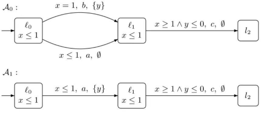
We consider injectively-labelled automata i.e., where two different edges have different labels (and no label is ε). Figure 1 shows two injectively-labelled timed automata that will be used to illustrate the constructions throughout the paper.
ℓ0 x ≤ 1 ℓ1 x ≤ 1 l2 x ≤ 1, a, ∅ x = 1, b, {y} x ≥ 1 ∧ y ≤ 0, c, ∅ A0: ℓ0 x ≤ 1 ℓ1 x ≤ 1 l2 x ≤ 1, a, {y} x ≥ 1 ∧ y ≤ 0, c, ∅ A1:
Fig. 1.Two timed automata
A valuation v is a mapping in RX
≥0. The effect of reset operations and time elapsing on valuations are described as follows. For R ⊆ X, the valuation v[R 7→ 0] maps each variable in R to the value 0 and agrees with v over X \ R. For valuation v and d ∈ R≥0, valuation v+d is defined by: ∀x ∈ X, (v+d)(x) = v(x)+ d. Constraints of C(X) are interpreted over valuations: we write v |= γ when the constraint γ is satisfied by v. The set of valuations satisfying a constraint γ is denoted by [[γ]].
Definition 3 (Semantics of TA). The semantics of a timed automaton A = (L, ℓ0, X, Σε, E, Inv) is a timed transition system SA = (Q, q0, →) where Q = L × (R≤0)X, q0= (ℓ0, 0) and → is defined by:
– either a delay move (ℓ, v)−−→ (ℓ, v + d) iff v + d |= Inv(ℓ),d
– or a discrete move (ℓ, v)−→ (ℓe ′, v′) iff there exists some e = (ℓ, γ, a, R, ℓ′) in E such that v |= γ, v′= v[R 7→ 0] and v′ |= Inv(ℓ′).
In order to ensure in a syntactic way that a move associated with a discrete transition e always leads to a configuration (ℓ′, v′) such that v′|= Inv(ℓ′), we may modify the initial timed automaton in the following way : any atomic constraint related to a clock x occurring in the invariant of ℓ′ is added to the guard of each transition arriving in ℓ′ which does not reset x. This transformation does not change the resulting transition system but makes some proofs simpler and in the sequel, we always assume that the timed automaton has this property.
Since our results are mainly based on the region automaton and some of its variants, we now recall the material needed.
2.3 Elementary zones of a timed automaton
Notations. A zone is a subset of (R≥0)X defined by a conjunction of atomic clock constraints of the form x ⊲⊳ h or x − y ⊲⊳ h, where x and y are clocks in X, h ∈ N and ⊲⊳∈ {<, ≤, ≥, >}. In particular, if γ is a clock constraint in C(X), then the set [[γ]] is a zone. Constraints of the form x − y ⊲⊳ h are usually called
diagonal constraints. The future of a zone Z is defined by f ut(Z) = {v + d |
v ∈ Z, d ∈ R≥0}. A zone Z satisfies a constraint γ ∈ C(X), written Z |= γ, if all valuations in Z satisfy γ. For k ∈ N, a k-zone is a zone for which no atomic clock constraint in its definition involves a constant greater than k.
Elementary zones. Recall [4] that, if m is the maximal constant appearing in atomic formulas x ⊲⊳ h of A, an equivalence relation with finite index can be defined on clock valuations, leading to a partition of (R≥0)X, with the following property: two equivalent valuations have the same behaviour under progress of time and reset operations, with respect to the constraints. In the original definition, an element of the partition is specified by a pair ({Ix}x∈X, ∝) where Ixis an interval in the set {{0}, ]0, 1[, {1}, . . . , {m}, ]m, +∞[} and ∝ is a relation on the subset of clocks x such that Ix6=]m, +∞[ defined by x ∝ y ≡ f ract(x) ≤ f ract(y).
Note that the property related to the behaviour of the systems holds for any partition which refines the above partition. In this paper, we define a fam-ily of refining partitions PK,g for K ≥ m + 1 and g ∈ N \ {0}. whose ele-ments are called elementary zones. The constant g is called the granularity and PK,g is called a g-grid. For such a partition the interval Ix belongs to the set {{0}, ]0,1 g[, { 1 g}, ] 1 g, 2 g[. . . , {K − 1 g}, ]K − 1 g, K[, [K, +∞[} (instead of keeping {K} separately). As before, we also specify the ordering on the fractional parts w.r.t.
g for all clocks x (i.e. the value δ ∈ [0,1g[ such that ∃i, x = gi+ δ) with valuation less than K. We include the case K = +∞.
When K is finite, reachability can be decided by the usual method applied on these partitions; however we consider [K, ∞[ (rather than the usual ]K, ∞[) as the last interval for topological reasons explained later. The partition K = +∞ is used here as a tool for our expressiveness results.
x y Z1 Z2 0 1 2 3
Fig. 2.Partition of (R+)2 with granularity g = 1 and K = 3
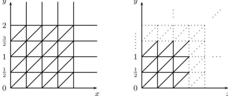
Figures 2 and 3 represent different partitions for the set of two clocks X = {x, y}. The horizontal and vertical lines correspond to the possible intervals Ix and Iy whereas the diagonal lines specify the ordering of fractional parts.
Figure 2 is associated with g = 1 and K = 3. For this example, elementary zones Z1 and Z2 are described as follows: Z1: (2 < x < 3) ∧ (1 < y < 2) ∧ (0 < f rac(y) < f rac(x)) or equivalently, (2 < x < 3) ∧ (1 < y < 2) ∧ (x − y > 1) and Z2 : (x ≥ 3) ∧ (1 < y < 2). Figure 3 (left) is associated with g = 2 and K = 2 while figure 3 (right) is associated with g = 2 and K = +∞. The dotted lines of this figure mean that the pattern is infinitely repeated.
x y 0 1 2 1 3 2 2 x y 0 1 2 1
If Z and Z′are elementary zones, Z′is a time successor of Z, written Z ≤ Z′, if for each valuation v ∈ Z, there is some d ∈ R≥0such that v + d ∈ Z′. For each elementary zone Z, there is at most one elementary zone such that (i) Z′is a time successor of Z, (ii) Z 6= Z′and (iii) there is no time successor Z′′different from Z and Z′ such that Z ≤ Z′′≤ Z′. When it exists, this elementary zone is called the immediate time successor of Z and denoted by succ(Z). From the definition of elementary zones as equivalent classes consistent with reset operations, the reset can be extended to elementary zones, so that Z[R 7→ 0] is the elementary zone containing any v[R 7→ 0], for v ∈ Z.
Standard topological notions on (R≥0)n apply to zones. Moreover, due to the particular form of the constraints, the topological closure of any elementary zone has a minimal element.
For a timed automaton A, a constant K and a granularity g, we call region a pair (ℓ, Z), where ℓ is a location of A and Z an elementary zone of (R≥0)X. We now give a description for regions, which distinguishes closed and
time-open descriptions. It is equivalent to the original one but more convenient for
our proofs and it fits both cases, whether K is finite or infinite.
Definition 4 (Region description w.r.t. constant K and granularity g).
A time-closed description of a region r is given by:
– ℓr the location of r,
– minr ∈ NXg with ∀x, minr(x) ≤ K, the minimal vector of the topological
closure of r,
– ActXr= {x ∈ X | minr(x) < K} the subset of relevant clocks,
– the number sizerof different fractional parts for the values of relevant clocks
in the NActXr
g grid, with 1 ≤ sizer≤ M ax(|ActXr|, 1) and the onto mapping ordr: X 7→ {1, . . . , sizer} giving the ordering of the fractional parts.
By convention, ∀x ∈ X \ ActXr, ordr(x) = 1.
Then r = {(ℓr, minr+ δ) | δ ∈ RX≥0 and ∀x, y ∈ ActXr [ordr(x) = 1 ⇔ δ(x) = 0] ∧ δ(x) < 1/g ∧ [ordr(x) < ordr(y) ⇔ δ(x) < δ(y)]}
A time-open description of a region r is defined with the same attributes (and conditions) as the time-closed one with:
r = {(ℓr, minr+ δ + d) | ∃ d ∈ R>0 ∧ ∀x ∈ ActXr, d(x) = d ∧ δ(x) + d < 1/g ∧ ∀x /∈ ActXr, d(x) = 0}.
The set [X]ris the set of equivalence classes of clocks w.r.t. their fractional parts,
i.e. x and y are equivalent iff ordr(x) = ordr(y).
Thus, a open region corresponds to an immediate time successor of a time-closed region and the decomposition of a valuation in a time-open region as minr+ δ + d is unique if minr+ δ belongs to the previous time-closed region. This property is used in the sequel.
Also remark that minr ∈ r except if there is a single class of clocks relative/ to r (for instance if the corresponding zone is a singleton). Of course, when K = +∞, the part about relevant clocks, for which the value is less than K,
can be omitted (since ActXr = X). The hypothesis K = +∞ makes some proofs simpler, because the extremal case where a clock value is greater than K is avoided, and it can be lifted afterward. Furthermore when K is finite, some regions admit both time-open and time-closed descriptions (for instance a region associated with zone Z2in fig. 3), whereas when K = +∞, a region admits a single description, so that time elapsing leads to an alternation of time-open regions (where time can elapse) and time-closed ones (where no time can elapse). Furthermore in this case, the representation of a valuation in a time-open region can be written minr+ δ + d with d a (scalar) duration.
2.4 Region automaton and class automaton of a TA.
For a timed automaton A, a constant K and a granularity g, the region auto-maton R(A)g,K is a finite automaton, the states of which are regions. These regions are built inductively from the initial one (ℓ0, 0) by the following trans-itions over the set of labels {succ} ∪ Σε:
– (ℓ, Z)−−−→ (ℓ, succ(Z)) if succ(Z) |= Inv(ℓ) andsucc
– (ℓ, Z)−→ (ℓa ′, Z′) if there is a transition (ℓ, γ, a, R, ℓ′) ∈ E such that Z |= γ and Z′= Z[R 7→ 0], with Z′ |= Inv(ℓ′).
A region r = (ℓ, Z) is said to be maximal in R(A)g,K with respect to ℓ if no succ-transition is possible from r. In the sequel, the topological properties of r are implicitly derived from those of Z. We write r for the topological closure of r, and recall that minr denotes the minimal vector of r.
We also consider another automaton, called the class automaton, in which the states, called classes, are of the form (ℓ, Z), where Z is a zone. In this case, the automaton is built from the initial class (ℓ0, f ut(0) ∩ Inv(ℓ0)) by the follow-ing transitions:
(ℓ, Z1)−→ (ℓa ′, Z2) if there exists (ℓ, γ, a, R, ℓ′) ∈ E such that Z1∩ [[γ]]6= ∅, and Z2= f ut((Z1∩ [[γ]])[R 7→ 0]) ∩ Inv(ℓ′).
While this construction does not always yield a finite number of classes, it is now well known [12] that for a timed automaton without diagonal constraints (as is our case), replacing each zone Z from the previous construction by its K-approximation (ApproxK(Z), the smallest K-zone containing Z), we obtain a finite automaton such that any configuration belonging to a zone is strongly timed bisimilar to a reachable configuration (see also the discussion of the next paragraph). This method is usually implemented in tools like Uppaal [25] or Kronos [28] for on-the-fly verification, with each zone represented by a Differ-ence Bounded Matrix [18].
2.5 Reachability
For a region r of R(A)g,K, not all configurations of r are reachable. Nevertheless, by induction on the reachability relation, the following property can be shown: for any region r of R(A)g,K, there is a region reach(r) with respect to the g-grid and constant K = ∞ such that
– (i) reach(r) ⊂ r,
– (ii) each configuration of reach(r) is reachable and
– (iii) if reach(r) admits a time-open description then this is also the case for r, else r admits a time-closed description.
As a consequence, we have: ∀x ∈ ActXr, minreach(r)(x) = minr(x) and ∀x ∈ X \ ActXr, minreach(r)(x) ≥ K and ordr restricted to ActXr is identical to ordreach(r).
Consider now the relation R defined by (ℓ, v) R (ℓ, v′) iff ∀x ∈ X, v′(x) = v(x) ∨ (v(x) ≥ K ∧ v′(x) ≥ K). It is a strong timed bisimulation relation. From the previous observations, we note that each configuration of a region is strongly timed bisimilar to a reachable configuration of this region. Thus speaking about reachability of regions is a slight abuse of notations. Note that the same property holds for the classes of the class automaton.
3
Characterizing TA bisimilar to Time Petri Nets
3.1 Time Petri Nets
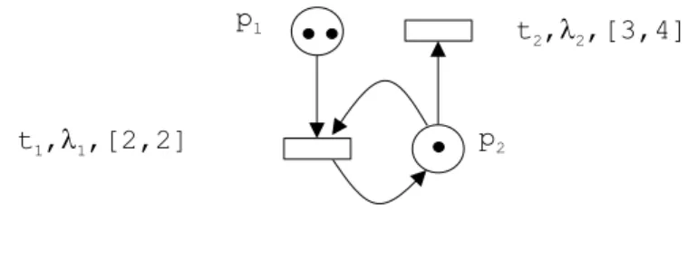
Introduced in [24], Time Petri Nets (TPNs) extend Petri nets by associating a (topological) closed time interval with each transition (see figure 4). The meaning of this interval is detailed after the definition.
Fig. 4.A labelled time Petri net
Definition 5 (Labeled Time Petri Net). A Labeled Time Petri Net N over Σε is a tuple (P, T, Σε,•(.), (.)•, M0, Λ, I) where:
– P is a finite set of places,
– T is a finite set of transitions with P ∩ T = ∅, – •(.) ∈ (NP)T is the backward incidence mapping, – (.)•∈ (NP)T is the forward incidence mapping, – M0∈ NP is the initial marking,
– Λ : T → Σε is the labeling function,
A TPN N is a g-TPN if for all t ∈ T , the interval I(t) has its bounds in Ng. We also use •t (resp. t•) to denote the set of places •t = {p ∈ P |•t(p) > 0} (resp. t• = {p ∈ P | t•(p) > 0}) as is common in the literature. The intended meaning of these notations will be clear from the context.
As usual, a marking M is a mapping in NP, with M (p) the number of tokens in place p. A transition t is enabled in a marking M iff M ≥•t. We denote by
En(M ) the set of enabled transitions in M . A configuration of a TPN is a pair
(M, ν) where M is a marking and the valuation ν is a mapping in (R≥0)En(M ), which describes the values of clocks implicitely associated with transitions en-abled in M . Roughly speaking, such a clock measures the time elapsed since the enabling of the corresponding transition as explained more precisely below.
An enabled transition t can be fired if ν(t) belongs to the interval I(t). The result of this firing is as usual the new marking M′ = M −•t + t•. Moreover, some valuations are reset and we say that the corresponding transitions are newly enabled. Different semantics are possible for this operation. In this pa-per, we choose persistent atomic semantics, which is different from the classical semantics [10,5], but equivalent when the net is bounded [6]. The predicate de-scribing when a transition t′ is newly enabled by the firing of transition t is defined by:
↑enabled(t′, M, t) = t′∈ En(M −•t + t•) ∧ (t′ 6∈ En(M )).
Thus, firing a transition is considered as an atomic step and the transition cur-rently fired behaves like the other transitions (ν(t) need not be reset when t is fired). In classical semantics, when firing a transition, disabling of the other transitions is checked after the consumption of tokens from input places and before the production of tokens to output places. Furthermore the clock asso-ciated with the fired transition is always reset. Observe that our results also hold for the classical semantics but we have chosen this one as it leads to more elegant constructions in sections 5 and 6. More precisely, the sufficient condi-tion is obtained by construccondi-tion of a bounded TPN and it has been proven that for bounded nets, both semantics are equivalent [6]. The necessary condition is based on lemmas 1 and 2 which do not depend on the triggering of clock reset in TPNs.
The set ADM(N ) of admissible configurations consists of the pairs (M, ν) such that ν(t) ∈ I(t)↓ for each transition t ∈ En(M ). Thus time can progress in a marking only until it reaches the first right endpoint of the intervals for all enabled transitions. For d ∈ R≥0, the valuation ν + d is defined by (ν + d)(t) = ν(t) + d for each t ∈ En(M ).
Definition 6 (Semantics of TPN). The semantics of a TPN N = (P, T, Σε, •(.), (.)•, M
0, Λ, I) is a TTS SN = (Q, q0, →) where Q = ADM(N ), q0= (M0, 0)
and → is defined by:
– either a delay move (M, ν)−−→ (M, ν + d)d
– or a discrete move (M, ν)−−−→ (M −Λ(t) •t+t•, ν′) where ∀t′∈ En(M −•t+t•), ν′(t′) = 0 if ↑enabled(t′, M, t) and ν′(t′) = ν(t′) otherwise,
iff t ∈ En(M ) and ν(t) ∈ I(t).
We simply write (M, ν)−→ to emphasise that a sequence of transitions w canw be fired. If Duration(w) = 0, we say that w is an instantaneous firing sequence. A net is said to be k-bounded if for each reachable configuration (M, ν) and for each place p, M (p) ≤ k.
Denoting ((M0(p1), M0(p2)), (ν0(t1), ν0(t2))) by ((2, 1), (0, 0)), the sequence ((2, 1), (0, 0)) −→ ((2, 1), (2, 2))2 t1
−→ ((1, 1), (2, 2)) t1
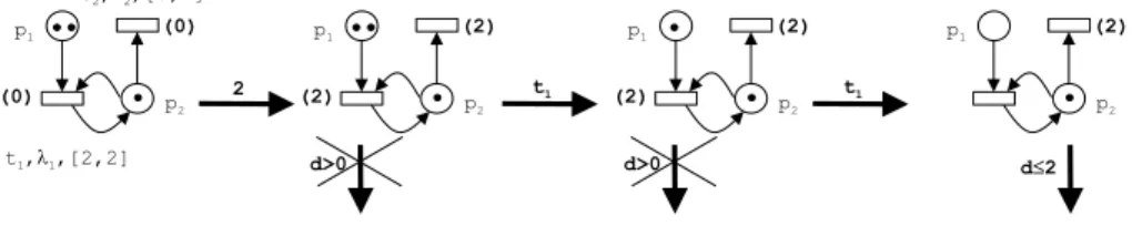
−→ ((0, 1), (−, 2)) is a firing sequence of the net of figure 4. Note that, due to the semantics, the first firing of t1 does not reset its clock even if the token in p2 is consumed and produced again. Note also that time cannot progress beyond time 2 as long as t1 remains fireable. Afterwards time can progress for at most 2 t.u. at which point t2 must fire (it could also fire before). This temporal feature is sometimes called an urgent behaviour in contrast to a lazy behaviour.
Fig. 5.An execution in a time Petri net
3.2 A characterization of TA bisimilar to TPNs
We aim at characterizing TA bisimilar to some TPN whatever the labelling of the TA. In fact to check this property is equivalent to test whether an associated injectively-labelled TA is bisimilar to some TPN. This is why we only consider injectively-labelled TA in the sequel.
TA include both lazy mechanisms since time elapsing can falsify the guard of an edge and urgent mechanisms since invariants may forbid time elapsing in some configurations. Hence a characterization of TA bisimilar to some TPN seems to be closely related to the absence of laziness features. In this paragraph, we first present two intuitive conditions for a TA to be bisimilar to a TPN which do not characterize this property before introducing the exact characterization. The first condition is obtained by observing that a transition (and more generally an instantaneous firing sequence) of a TPN cannot be disabled by time elapsing. Consequently, our first attempt to characterize this property is: “A TA is bisimilar to some TPN if time elapsing cannot falsify the guard of an edge
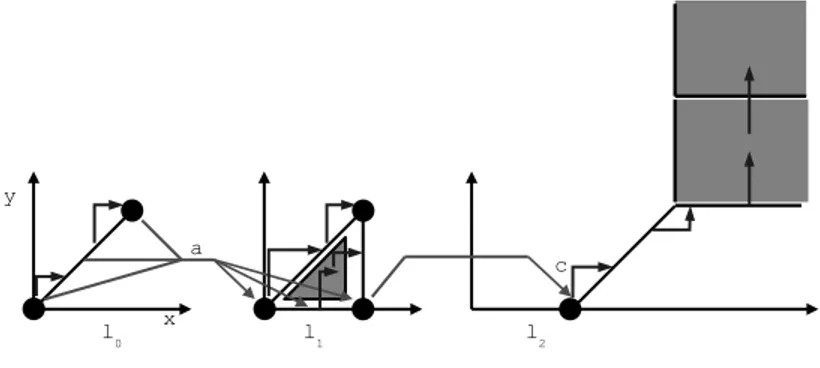
starting from the current location”. By virtue of the observation this condition is necessary. However it is not sufficient and the automaton A1 of figure 1 does not admit a bisimilar TPN whereas it fulfills this condition as can be checked on its region automaton represented in figure 6. The three parts of this figure (from left to right) represent respectively the reachable regions associated with locations ℓ0, ℓ1and ℓ2. Thin arrows represent time elapsing (thus staying in the same location) while thick (labelled) arrows represent discrete transitions from some (ℓ, Z) to another region (ℓ′, Z′). For instance, (ℓ0, 0 < x = y < 1) −→a (ℓ1, 0 < x < 1 ∧ y = 0)
Fig. 6.The region automaton of A1 (K = 2, g = 1)
The previous observation about the behaviour of a TPN may be sharpened and yields the following lemma useful for subsequent developments.
Lemma 1. Let (M, ν) and (M, ν + δ) be two admissible configurations of a
g-TPN with ν, δ ∈ REn(M )≥0 . Let w be an instantaneous firing sequence, then: (i) (M, ν)−w→ implies (M, ν + δ)−→w
(ii) If ν ∈ NgEn(M ) and δ ∈ [0, 1/g[En(M ) then (M, ν + δ)−→ implies (M, ν)w −w→
Proof. There are two kinds of transitions firing in w: those corresponding to a
firing of a transition (say t) still enabled from the beginning of the firing sequence and those corresponding to a newly enabled transition (say t′).
Proof of (i) Since t is firable from (M, ν), ν(t) ∈ I(t) ⊂ I(t)↑, so ν(t) + δ(t) ≥ ν(t) also belongs to I(t)↑. Since t ∈ En(M ) and (M, ν + δ) is reachable, ν(t) + δ(t) ∈ I(t)↓. Thus ν(t) + δ(t) ∈ I(t) and t is also firable from (M, ν + δ). Since t′ is newly enabled, 0 ∈ I(t′) and t′ is also firable when it occurs starting from (M, ν + δ).
Proof of (ii) The case of newly enabled transitions in w is handled as before. Now let t be firable in (M, ν + δ). Since t ∈ En(M ) and (M, ν) is reachable, ν(t) ∈ I(t)↓. Since ν(t)+δ(t) ∈ I(t)↑, (denoting by ef t(t) the minimum of I(t)↑), we have ef t(t) ≤ ν(t)+δ(t) but ef t(t) belongs to the g-grid, thus ef t(t) ≤ ν(t) ⇔
Taking into account this lemma, one can elaborate a slightly modified ver-sion of the first condition: “A TA is bisimilar to some TPN if given any two reachable configurations (l, v) and (l, v′) with v′ ≥ v and an edge e, then (l, v) −→⇒ (l, ve ′) −→”. For instance, Ae
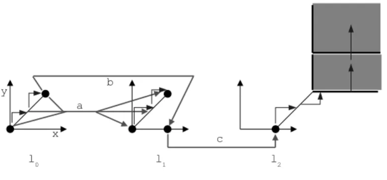
1 does not fulfill this condition (take (l1, (1, 0)),(l1, (1, 1)) and the edge labelled by c in figure 6). Unfortunately this condition is not necessary. The TA A0 of figure 1 does not fulfill this condition whereas there exists a TPN bisimilar to it (see figure 13 in section 5). Indeed take (l1, (1, 0)),(l1, (1, 1)) and the edge labelled by c and see its region automaton presented in figure 7 (with the same conventions as in figure 6).
Fig. 7.The region automaton of A0 (K = 2, g = 1)
The difference between the two automata w.r.t. the property to be checked is the existence of the reachable region (l1, x = 1 ∧ 0 < y < 1) whose topological closure includes the configuration (l1, (1, 0)). In fact, the exact characterization takes into account topological considerations as stated by the following theorem which also contains effectiveness and complexity results.
Theorem 1. Let A be a injectively-labelled timed automaton and R(A)1,K its
region automaton with a constant K strictly greater than any constant occurring in the automaton, then A is weakly timed bisimilar to a time Petri net iff for each region r of R(A)1,K and for each edge e from A,
(a) Every region r′ such that r′∩ r 6= ∅ is reachable (b)∀(ℓr, v) ∈ r, if (ℓr, v) e − → then (ℓr, minr) e − → (c)∀(ℓr, v) ∈ r, if (ℓr, minr) e − → then (ℓr, v) e − →.
Furthermore, if these conditions are satisfied then we can build a 1-bounded 2-TPN bisimilar to A whose size is linear w.r.t. the size of A and a 1-bounded 1-TPN bisimilar to A whose size is exponential w.r.t. the size of A.
We denote by T Awtb the corresponding subclass of timed automata.
Thus T Awtb is the maximal subclass of TA that are weakly timed bisimilar to a TPN. In [7], we have proposed a “syntactical” (proper) subclass of T Awtb which avoids to check this characterization.
The characterization of Theorem 1 is closely related to the topological closure of reachable regions: it states that any region intersecting the topological closure of a reachable region is also reachable and that a discrete step either from a region or from the minimal vector of its topological closure is possible in the whole topological closure. Consider again the two TA A0 and A1 in Figure 1. The automaton A0 admits a bisimilar TPN whereas A1 does not. Indeed, the region r = (ℓ1, x = 1 ∧ 0 < y < 1) is reachable. The guard of edge c is true in minr= (ℓ1, (1, 0)) whereas it is false in r.
The next sections are devoted to the proof of Theorem 1.
4
Proof of necessary condition for Theorem 1
4.1 From bisimulation to uniform bisimulation
As a first step, we prove that when a g-TPN and a TA are bisimilar, this relation can in fact be strengthened in what we call uniform bisimulation. Lemma 2 is the central point for the proof of necessity. It shows that bisimulation implies uniform bisimulation for the g-grid with K = ∞. Roughly speaking, uniform bisimulation means that a unique mechanism is used for every configuration of the topological closure of the region to obtain a bisimilar configuration of the net.
Lemma 2 (From bisimulation to uniform bisimulation). Let A be a timed
automaton bisimilar to some g-TPN N via some relation R and let R(A)g,∞ be
a region automaton of A. Then:
– if a region r belongs to R(A)g,∞ then any region included in r also belongs
to R(A)g,∞;
– for each region r, there exist a configuration of the net (Mr, νr) with νr ∈ NEn(Mr)
g and a mapping φr: En(Mr) → [X]r such that: • If r is time-closed, then for each δ ∈ RX
≥0 such that (ℓr, minr+ δ) ∈ r, (ℓr, minr+ δ) R (Mr, νr+ projr(δ)),
• If r is time-open, then for each δ ∈ RX
≥0, d ∈ R≥0 such that (ℓr, minr+ δ+ d) ∈ r, (ℓr, minr+ δ + d) R (Mr, νr+ projr(δ) + d),
where projr(δ)(t) = δ(φr(t)).
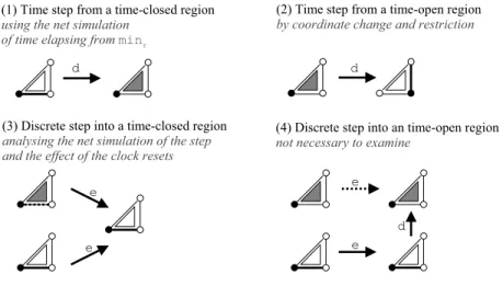
Proof. First note that the choice of a particular clock x in the class φr(t) is irrelevant when considering the value δ(x). Thus the definition of projris sound. The proof is an induction on the transition relation in the region automaton. The basis case is straightforward with {(l0, 0)} and {(M0, 0)}. The induction part relies on lemma 1, with 4 cases, according to the incoming or target region and to the nature of the step: 1. a time step from a time-closed region, 2. a time step from a time-open region, 3. a discrete step into a time-closed region, and 4. a discrete step into a time-open region.
1. A time step from a time-closed region (see figure 8(1)). Let r be a time-closed region in R(A)g,∞ and let us denote r′ = succ(r) the immediate
time successor of r. Let (ℓr, minr+ δ0) be some item of r. (ℓr, minr+ δ0) d −→ for some d > 0. Thus (by induction hypothesis) in N there is a step sequence of (Mr, νr+ projr(δ0))
d0t1...tndn
−−−−−−−→ with all transitions labelled by ǫ andPdk= d. Let dk be the first non zero elapsing of time. By application of lemma 1-(ii), the firing sequence t1. . . tk is fireable from (Mr, νr).
Let us choose (Mr′, νr′) the configuration reached by this sequence. By
ap-plication of lemma 1-(i), this firing sequence is also fireable from any (Mr, νr+ projr(δ)) bisimilar to (ℓr, minr+δ) ∈ r and it leads to (Mr′, νr′+projr′(δ)) (still
bisimilar to (ℓr, minr+δ)) where φr′ (resp. νr′) is equal to φr(resp. νr) for trans-itions always enabled during the firing sequence and φr′ (resp. νr′) is obtained by
associating the class of index 1 (resp. by associating the value 0) with the trans-itions newly enabled. Since (Mr′, νr′) let the time elapse and since N is a g-TPN,
we note that ∀t ∈ En(Mr′), νr′(t) + 1/g ∈ I(t)↓. Now let (ℓr, minr+ δ + d) ∈ r′,
one has ∀x ∈ X, δ(x) + d ≤ 1/g. Thus ∀t ∈ En(Mr′), projr′(δ(x)) + d ≤ 1/g,
which implies (Mr′, νr′+ projr′(δ))
d
−→ (Mr′, νr′ + projr′(δ) + d), this last
con-figuration being necessarily bisimilar to (ℓr, minr+ δ + d).
2. A time step from a time-open region (see figure 8(2)). Let r be an time-open region and let us denote r′ = succ(r). Note that r′⊂ r. Let us define Xmax
r the class [x]r with maximal index. We remark that minr′ = minr+ δ0 where if x ∈ Xmax
r then δ0(x) = 1/g else δ0(x) = 0. We choose (Mr′, νr′) =
(Mr, νr+ projr(δ0)). Let t ∈ En(Mr) and x ∈ φr(t) then φr′(t) = [x]r′ (letting
time elapse does not split the classes). So projrand projr′ are identical.
Now let (lr′, minr′+ δ) ∈ r′. (lr′, minr′+ δ) = (ℓr, minr+ δ0+ δ).
Now let d = δ(x) for x belonging the class of index 1 in [Xr]. Then (ℓr, minr+ δ0+ δ) = (ℓr, minr+ δ′+ d) where if x ∈ Xrmax then δ′(x) = 1/g − d else δ′(x) = δ(x) − d. (ℓ
r, minr+ δ′+ d) is bisimilar to (Mr, νr+ projr(δ′) + d) = (Mr, νr+ projr(δ′+ d)) = (Mr, νr+ projr(δ1+ δ)) = (Mr, νr+ projr(δ1) + projr(δ)) = (Mr′, νr′+ projr′(δ))).
For this step, we have not used the characteristics of time Petri nets. 3. A discrete step into a time-closed region (see figure 8(3)). Case a. We first consider the case where r is a time-closed region.
Let (ℓr, minr+δ0) be some element of r. Suppose that (ℓr, minr+δ0) e − → (l′, v′+ δ′
0) with ∀x ∈ R(e), v′(x) = δ′0(x) = 0, ∀x /∈ R(e), v′(x) = minr(x) ∧ δ′
0(x) = δ0(x). Then in N there is an instantaneous firing sequence (Mr, νr+ projr(δ0))
w
−→ labelled by e. Due to lemma 1, this firing sequence is also fireable from any (Mr, νr+ projr(δ)) bisimilar to (ℓr, minr+ δ) ∈ r. By bisimilarity, (ℓr, minr+δ)
e
−→ for any (ℓr, minr+ δ) ∈ r. Let r′ be the region including (ℓ′, v′+δ′
0), then any configuration of r′is reachable by this discrete step. Note that ℓr′ = l′ and minr′ = v′.
From (Mr, νr+ projr(δ)), the sequence w leads to some (M′, ν′) bisimilar to (ℓr′, minr′ + δ′)). We now show how to define Mr′, νr′ and φr′. First
Mr′ = M′. Second, νr′(t) = νr(t) for transitions t always enabled during the firing sequence and νr′ = 0 otherwise. At last, φr′ is obtained from φr
Fig. 8.The different cases of the proof
as follows. Let t be a transition newly enabled during the firing sequence, then φr′(t) is associated to the class of index 1. Let t be a transition always
enabled during the firing sequence. There are two cases to consider for φr′(t):
if there is a x ∈ φr(t) not reset, then φr′(t) = |x]r′ otherwise φr′(t) is the
class of maximal index which precedes φr(t) and contains a clock not reset or else the class of index 1. The two last affectations are sound since, it means that whatever, before the firing of w, the fractional value of the implicit clock associated with t between the fractional value of the new clock corresponding to t and the fractional value of a clock of φr(t), the firing sequence w leads to bisimilar configurations (as being bisimilar to the same configuration of the automaton).
Case b. The case where r is a time-open region is handled in a similar way. Let (ℓr, minr+δ0+ d0) be some element of r. Suppose that (ℓr, minr+δ0+ d0)
e −
→ (ℓ′, v′+ δ′
0) with ∀x ∈ R(e), v′(x) = δ0′(x) = 0, ∀x /∈ R(e), v′(x) = minr(x) ∧ δ0′(x) = δ0(x) + d0. Then in N there is an instantaneous firing sequence (Mr, νr+ projr(δ0) + d0)−w→ labelled by e. Due to lemma 1, this firing sequence is also fireable from any (Mr, νr+ projr(δ) + d) bisimilar to (ℓr, minr+ δ + d) ∈ r. By bisimilarity, (ℓr, minr+δ + d)
e −
→ for any (ℓr, minr+ δ + d) ∈ r. Let r′ be the region including (l′, v′+ δ′0), then any configuration of r′ is reachable by this discrete step. Note that l
r′ = l′ and
minr′ = v′.
From (Mr, νr+projr(δ)+d), the sequence w leads to some (M′, ν′) bisimilar to (lr′, minr′ + δ′)). We now show how to define Mr′, νr′ and φr′. First
Mr′ = M′. Second, νr′(t) = νr(t) for transitions t always enabled during the firing sequence and νr′ = 0 otherwise. At last, φr′ is obtained from φr as follows. Let t be a transition newly enabled during the firing sequence, then φr′(t) is associated to the class of index 1. There are two cases to consider
for φr′(t): if there is a x ∈ φr(t) not reset, then φr′(t) = |x]r′ otherwise φr′(t)
is the class of maximal index which precedes φr(t) and contains a clock not reset or else the class of index 1. The two last affectations are sound since, it means that whatever, before the firing of w, the fractional value of the implicit clock associated with t between the fractional value of the new clock corresponding to t and the fractional value of a clock of φr(t), the firing sequence w leads to bisimilar configurations (as being bisimilar to the same configuration of the automaton).
4. A discrete step into a time-open region (see figure 8(4)). In order to reach a time-open region by a discrete step, the corresponding transition must start from a time-open region and must not reset any clock. Let (ℓr, minr+ δ + d) ∈ r and (ℓr, minr+ δ + d)
e −
→ (l′, min
r+ δ + d). Here we have used the hypothesis that no clock is reset. Then there is a firing sequence (Mr, νr+ projr(δ) + d)−w→ labelled by e. Due to the lemma 1, (Mr, νr+projr(δ))
w
−→. (ℓr, vr+δ) is bisimilar to (Mr, νr+ projr(δ)). Thus (ℓr, minr+ δ)
e − → (l′, min r+ δ) d −→ (l′, min r+ δ + d). Then this region can be reached via a discrete step into a time-closed region followed by a time step. So we do not need to examine this case. ⊓⊔
4.2 Proof of Necessity
The fact that conditions (a), (b) and (c) of Theorem 1 hold for R(A)g,∞is now straightforward:
(a) This assertion is included in the inductive assertions.
(b) Let r be a region, let (ℓr, minr+ δ) ∈ r be a configuration with δ ∈ [0, 1/g[X, then ∃(M, ν) ν ∈ NEn(M )
g bisimilar to (ℓr, minr) and (M, ν + δ′) with δ′∈ [0, 1/g[En(M ) bisimilar to (ℓ
r, v + δ). Suppose that (ℓr, minr+ δ) e − →, then (M, ν + δ′)−w→ with w an instantaneous firing sequence and label(w) = e. Now by lemma 1-(ii), (M, ν)−w→, thus (ℓr, minr)
e − →.
(c) Let r be a region, and (ℓr, minr+ δ) ∈ r with δ ∈ [0, 1/g]X thus ∃(M, ν) bisimilar to (ℓr, minr) and (M, ν + δ′) with δ′ ∈ [0, 1/g]En(M ) bisimilar to (ℓr, minr+ δ). Suppose that (ℓr, minr)
e
−→, then (M, ν)−w→ with w an instantan-eous firing sequence and label(w) = e. By lemma 1-(i), we have (M, ν + δ′)−w→, thus (ℓr, minr+ δ)−→.e
In order to complete the proof, we successively show that if the conditions are satisfied in R(A)g,∞ for some g, they also hold for R(A)1,∞ (lemma 3), and finally that they are satisfied in the standard region automaton R(A)1,K, with a finite constant K, sufficiently large (lemma 4). Recall (section 2.2) that any atomic constraint related to a clock x occurring in the invariant of a location is added to the guard of each incoming transition which does not reset x.
Lemma 3 (about the conditions and the grid). Let A be a timed
maton and g > 0 in N. If conditions (a),(b),(c) are satisfied in the region auto-maton R(A)g,∞, then they are satisfied in R(A)1,∞.
Proof. From the definition of regions, a region r of R(A)1,∞is a finite union of regions of R(A)g,∞ (say r = Si=1..kri). Thus r = Si=1..kri which proves the implication for (a).
Assume that (b) is satisfied by R(A)g,∞. Let (ℓr, minr+ δ + d) ∈ r be a region of R(A)1,∞ and assume (ℓr, minr+ δ + d)
e −
→. We define δ′ by δ′(x) = δ(x)/g. Then since A has integer constraints (ℓr, minr+ δ′+ d/g) −→. Moreover thise configuration belongs to r and then to a region r′ ∈ R(A)
g,∞ whose minimal vector is minr. Then applying (b), we obtain (ℓr, minr)−→.e
Assume that (c) is satisfied by R(A)g,∞. Let (ℓr, v) ∈ r where r is a region of R(A)1,∞and assume (ℓr, minr)
e −
→. Then there is an increasing path among the minimum vectors of regions of R(A)g,∞ all included in r. This path is such that any two consecutive elements belong to the closure of some region; it starts at (ℓr, minr) and finishes at (ℓr, minr∗) such that (ℓr, v) ∈ r∗ (with r∗ a region of
R(A)g,∞). Thus applying iteratively (c) yields (ℓr, v) e −
→. ⊓⊔
Lemma 4 (about the conditions and the constant K). Let A be a timed
automaton. If conditions (a),(b),(c) are satisfied in R(A)1,∞, then they hold in
the region automaton R(A)1,K, for some finite constant K.
Proof. Let r be a region in R(A)1,K where K is greater than the maximal con-stant in A and reach(r) the associated region of R(A)1,∞. Note that ℓreach(r)= ℓr and that ∀x ∈ ActXr, minreach(r) = minr and ∀x ∈ X, minreach(r)≥ minr. Suppose that reach(r) is closed (resp. open) then r admits a time-closed (resp. time-open) description where the ordr and ordreach(r) mappings are identical for clocks in ActXr. Thus ∀(ℓr, v) ∈ r, ∃(ℓr, v′) ∈ reach(r) such that ∀x ∈ ActXr, v′(x) = v(x).
Now take a convergent sequence limi→∞(ℓr, vi) = (ℓr, v) with (ℓr, vi) ∈ r so that (ℓr, v) ∈ r. Then the corresponding sequence {(ℓr, vi′)} being bounded admits an accumulation point (ℓr, v′) ∈ r. It is routine to show that (ℓr, v) and (ℓr, v′) belong to the same region in R(A)1,K. This proves that condition (a) for R(A)1,∞implies condition (a) for R(A)1,K.
Assume that (b) is satisfied by R(A)1,∞. Let (ℓr, v) ∈ r be a reachable region of R(A)1,K and (ℓr, v)
e −
→. Let reach(r) be the associated reachable region (as ex-plained in section 2.5) of R(A)1,∞then ∃(ℓr, v′) ∈ reach(r) strongly time bisim-ilar to (ℓr, v), thus (ℓr, v′)
e −
→. Using condition (b), (ℓr, minreach(r)) e − →. Since (ℓr, minreach(r)) is strongly time bisimilar to (ℓr, minr), we have (ℓr, minr)−→.e Assume that (c) is satisfied by R(A)1,∞ and consider (ℓr, v) ∈ r where r is a region of R(A)1,K and (ℓr, minr)
e −
→. Again let reach(r) be the associated reachable region of R(A)1,∞, then ∃(ℓr, v′) ∈ reach(r) strongly time bisim-ilar to (ℓr, v). Since (ℓr, minreach(r)) is strongly time bisimilar to (ℓr, minr), (ℓr, minreach(r))
e −
→. Thus using condition (c), (ℓr, v′) e −
→. By bisimilarity, we
5
Sufficient condition: first construction
Starting from a timed automaton A satisfying the conditions of Theorem 1, we build a 2-TPN bisimilar to A. We describe the construction and give the proof of correctness.
For the figures corresponding to all constructions, all edges are weighted by 1. Omitted labels for transitions stand for ε. A firing interval [0, 0] is indicated by a blackened transition and intervals [0, ∞[ are omitted. A double arrow between a place p and a transition t indicates that p is both an input and an output place for t.
5.1 Construction
First remark that any constraint of the form x < c occurring in an invariant of A may be safely omitted. If it would forbid the progress of time in some configuration, then the associated region would be a maximal time-open region r. Due to condition (a), r is reachable but since r is time-open, r ∩ succ(r) 6= ∅, so that succ(r) is reachable which contradicts the maximality of r.
• Tx<h Fx<h changex<h [h −1 2, h − 1 2] Rnextx i Rnextx i+1 Rinit reset1 x<h reset2x<h initx<h • Tx≤h Fx≤h changex≤h [h +1 2, h + 1 2] Rnextx i Rnextx i+1 Rinit reset1x≤h reset2x≤h initx≤h
Fig. 9.Subnets for x < h (with h > 0) and x ≤ h in guards
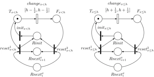
Clock constraints. The atomic constraints associated with a clock x are ar-bitrarily numbered from 1 to n(x) where n(x) is the number of such condi-tions. When x ≤ h occurs in at least one transition and in at least one invari-ant, we consider it as two different conditions. Then we add places Rinit and (Rnextx
i)i≤n(x)+1 for the reset operations. We build a subnet for each atomic constraint x ⊲⊳ h occurring in a transition of the TA, and one for each condition x ≤ h occurring in an invariant. Figure 9 shows the subnets corresponding to x < h (with h > 0) on the left and x ≤ h on the right, while Figure 10 shows
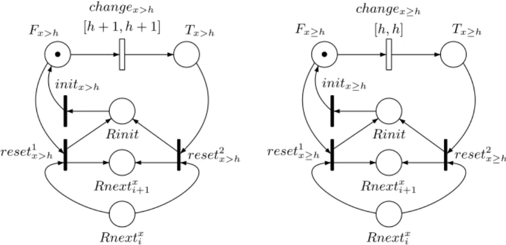
the subnets for x > h on the left and x ≥ h (with h > 0) on the right, in the case where the constraint has number i. Figure 11 shows the subnet for invariant x ≤ h.
Since constant 1
2 appears in interval bounds, the resulting TPN is a 2-TPN.
• Fx>h Tx>h changex>h [h + 1, h + 1] Rnextx i Rnextx i+1 Rinit reset1x>h reset2x>h initx>h • Fx≥h Tx≥h changex≥h [h, h] Rnextx i Rnextx i+1 Rinit reset1 x≥h reset2x≥h initx≥h
Fig. 10.Subnets for x > h and x ≥ h (with h > 0) in guards
• F Reachx≤h T Reachx≤h reachx≤h [h, h] Rnextx i Rnextx i+1 Rinit reset1 x≤h reset2x≤h initx≤h
Fig. 11.Subnet for x ≤ h in an invariant
Locations and edges. With each location ℓ of the automaton, we associate an eponymous place ℓ. The place ℓ is initially marked iff the location ℓ is the initial one. The invariant Inv(ℓ) is tested with the subnets corresponding to its atomic constraints:
– if condition x ≤ h (with h > 0) occurs in the invariant, then we add a transition stopx≤hℓ , with both ℓ and T Reachx≤has input and output places, and interval [0, 0],
– if condition x ≤ 0 occurs in the invariant, we simply add a transition stopℓ with ℓ as only input and output place, and also interval [0, 0].
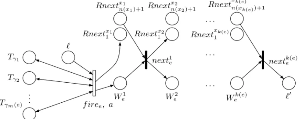
To simulate an edge e = (ℓ, γ, a, R, ℓ′), we must test the atomic constraints from γ = γ1∧ . . . ∧ γm(e), using the places corresponding to true in the asso-ciated subnets, and reset successively all the clocks in R = {x1, . . . , xk(e)} by instantaneous transitions. This is done by the subnet in Figure 12, which must be connected to some subnets like those of Figure 9, 10 or 11.
Tγ1 Tγ2 Tγm(e) .. . . . . . . . . . . ℓ W1 e We2 Wek(e) Rnextx1 1 Rnextx1 n(x1)+1 Rnext x2 n(x2)+1 Rnextx2 1 Rnext xk(e) 1 Rnextxk(e) n(xk(e))+1 ℓ′ f iree, a next1 e nextk(e)e
Fig. 12.The subnet for edge e = (ℓ, γ = γ1∧ . . . ∧ γm(e), a, R = {x1, . . . , xk(e)}, ℓ′)
This construction is illustrated in figure 13 for the timed automaton A0from figure 1 with some simplifications related to this particular timed automaton. More precisely, places F Reachx≤1 and Fx≥1 (resp. T Reachx≤1 and Tx≥1) have been merged. Moreover since x is never reset in A0 the corresponding parts in the TPN are omitted.
First note that the subnet associated to the constraint y ≤ 0 switches the condition to false (marking Fy≤0) when the implicit value of y maintained in the net reaches 1/2. This translation thus seems less constrained than the original condition, so we explain how we prove that it is nevertheless sound. Let r be the region corresponding to the current configuration (ℓ, v) of the automaton simulated by the net. If the net is able to simulate a discrete step of the auto-maton, we prove that in the configuration (ℓ, minr) of the automaton, this step is also possible. Thus by condition (c), the step is also possible from (ℓ, v). On the other hand, if a discrete step is possible for (ℓ, v) in the automaton, we show that this step can also be simulated in the net using both conditions (b) and (c) and the following fact: ∀x ∈ X, ∃(ℓr, v′), (ℓr, v′′) ∈ r such that v′(x) = ⌊v(x)⌋ and v′′(x) = ⌈v(x)⌉. The subnet associated to the atomic constraint x ≤ 1 oc-curing in the invariant of ℓ0leads to transition inv0(not modifying the marking)
• • • Rnext [1/2, 1/2] Rinit inity≤0 c, [0, +∞[ l2 ℓ1 Fx≥1 Ty≤0 F y≤0 ℓ0 a, [0, +∞[ b, [0, +∞[ Tx≥1 [1, 1] stopx≤1ℓ0 Fig. 13.A 2-TPN bisimilar to A0
which is fireable as soon as the simulated value of x reaches 1 and the place ℓ0 is marked. Thus time cannot progress except if the location is left.
5.2 Correctness proof
We decompose the reachable configurations (and markings) into intermediate ones (some Wi
e is marked) and permanent ones (some ℓ is marked). An easy induction shows that in permanent configurations (M, ν) the enabled timed transitions relative to a clock are “synchronized”: ν(changec) = ν(changec′) =
ν(reachc′′) as soon as c, c′, c′′ relates to the same clock x. We define ν(x) as
this common value if at least one such transition is enabled and otherwise ν(x) = K(x) where K(x) is the maximal value relative to clock x occuring in the net N . Furthermore from any intermediate configuration (M, ν), the beha-viour of the net is quasi-deterministic until it reaches a permanent configuration: there are only instantaneous firing sequences (i.e. no time step) and the finite maximal ones lead to permanent configurations. These permanent configura-tions (say (Mnext, νnext)) have the same marked place ℓ and the same values νnext(x). They may only differ depending on whether some transitions related to a condition switch have been fired.
It is also obvious that once some f ireeis fired, the construction ensures the existence of a “resetting” sequence which reinitializes the subnets associated to the clocks to be reset.
Bisimulation relation. We now define the relation R between reachable
config-urations of the automaton A and the net N . Let us define (ℓ, v)R(M, ν) iff: – either M is a permanent marking and M (ℓ) is marked and if ν(x) < K(x)
– or M is an intermediate marking leading to some permanent (Mnext, νnext) and (ℓ, v)R(Mnext, νnext). This definition is sound due to the common fea-tures of the different (Mnext, νnext).
It remains to prove that R is a bisimulation, which is done in the next lemma. Lemma 5. The relation R defined above is a weak timed bisimulation.
Proof. We first consider moves from A.
Case 1: (ℓ, v)−→ (ℓe ′, v′).
We prove that (M, ν)−→ with σ labelled by e. At first, σ begins by σσ ′ which con-sists to fire all the changecfireable leading to some (M′, ν′) (with (ℓ, v)R(M′, ν′)). Now we prove that (M′, ν′) f iree
−−−→. By definition of R, M (ℓ) is marked. Let c be a condition occuring in the guard of e.
If c = [x ≥ a] then v(x) ≥ a which implies ν(x) ≥ a and that Tx≥a is marked (possibly with the help of σ′).
If c = [x > a] then let r be the region to which (ℓ, v) belongs. minr(x) = ⌊v(x)⌋. Using condition (b), (l, minr)
e −
→. Thus v(x) ≥ minr(x) ≥ a + 1 which implies ν(x) ≥ a + 1 and that Tx>a is marked (possibly with the help of σ′).
If c = [x ≤ a] then v(x) ≤ a which implies ν(x) ≤ a and that Tx≤a is marked (remember that changex≤afires when ν(x) = a + 1/2).
If c = [x < a] then let r be the region to which (ℓ, v) belongs. Then there exists (ℓ, v1) ∈ r with v1(x) = ⌈v(x)⌉. Using condition (b) and then (c), (l, v1)
e − →. Thus v(x) ≤ v1(x) ≤ a − 1 which implies ν(x) ≤ a − 1 and that Tx<ais marked (remember that changex<afires when ν(x) = a − 1/2).
Thus f ireeis fireable from (M′, ν′). We complete σ by the “resetting” sequence leading to a configuration bisimilar to (ℓ′, v′)
If M is an intermediate marking, we have to fire a sequence leading to some (Mnext, νnext) and perform the previous simulation.
Case 2: (ℓ, v)−→ (ℓ, v + d)d
If M is an intermediate marking, again we fire an instantaneous sequence leading to some (Mnext, νnext) still bisimilar to (ℓ, v) and perform the following simulation for the case when M is permanent.
We must determine which transitions could prevent d time units to elapse: either change or stop transitions. When after d′ < d time units, a change trans-ition prevents time elapsing, it is fired leading to another permanent marking bisimilar to (ℓ, v + d′). The only possible stop transitions that could prevent time elapsing correspond to conjuncts of the form x ≤ a belonging to the invariant of ℓ. This means that v(x) + d ≤ a. Thus from (M, ν), we let a time d elapse inter-leaved with possible firings of change transitions. The stop transitions associated with ℓ will be possibly firable but only at the end of this step sequence.
Conversely, we consider moves from N . Case 3: (M, ν)−→ (Mt ′, ν′)
Thus we only to need to examine the case of f iree (M is then a perman-ent marking). Let r be the region to which (ℓ, v) belongs. We will show that (ℓ, minr)
e −
→. Then by condition (c), we will obtain that (ℓ, v)−→.e Let c be a condition occuring in the guard of e.
If c = [x ≥ a] then Tx≥a is marked which implies that ν(x) ≥ a and then v(x) ≥ a, thus minr(x) = ⌊v(x)⌋ ≥ a.
If c = [x > a] then then Tx>a is marked which implies that ν(x) ≥ a + 1 and then v(x) ≥ a + 1 thus minr(x) = ⌊v(x)⌋ ≥ a + 1 > a
If c = [x ≤ a] then Tx≤ais marked which implies that ν(x) ≤ a + 1/2 and then v(x) ≤ a + 1/2 thus minr(x) = ⌊v(x)⌋ ≤ a
If c = [x < a] then Tx<ais marked which implies that ν(x) ≤ a − 1/2 and then v(x) ≤ a − 1/2 thus minr(x) = ⌊v(x)⌋ ≤ a − 1 < a
So (ℓ, v)−→ (ℓe ′, v′) for some (ℓ′, v′). By construction of N and definition of R, (ℓ′, v′)R(M′, ν′).
Case 4: (M, ν)−→ (M, ν + d)d
An intermediate marking cannot let time elapse. Thus M is a permanent marking. Let x ≤ a belonging to the invariant of ℓ. Then a 6= 0, otherwise from (M, ν), transition stopℓ must be fired and time may not elapse. Similarly since stopx≤aℓ is only possibly fireable from (M, ν + d), it follows that ν(x) + d ≤ a, thus v(x) + d ≤ a.
Consequently (ℓ, v)−→ (ℓ, v + d) and obviously (ℓ, v + d)R(M, ν + d).d ⊓⊔
6
Sufficient condition: second construction
When the conditions on the injectively-labelled timed automaton A are satisfied, we now build a 1-TPN N which is weakly timed bisimilar to A.
6.1 Construction
The construction of the TPN contains a partial replication of both the region automaton of A and its class automaton. Recall that we consider K = m + 1, where m is the maximal constant for A. There is first a subnet for each clock x, in which only the integral parts of x appear in the places (but with a fractional part that can reach 1).
• . . . hx 0 tx0 hx1 [1, 1] tx 1 [1, 1] tx K−1 [1, 1] hx K
Fig. 14.Subnet for clock x
Then we add one place C for each class C = (ℓ, Z) of the class automaton, with the initial class marked. Now let e = (ℓ, g, a, R, ℓ′) be a transition of A. For
each pair (v, v′) of clock valuations in NX, with v, v′ ≤ −→K , we build a subnet (see figure 15) which simulates the transition (ℓ, v) −→ (ℓe ′, v′), where we have v′(x) = 0 if x ∈ R and v′(x) = v(x) otherwise. Let C1= (ℓ, Z1), . . . , Ck= (ℓ, Zk) be the subset of classes such that ∃v′′ ∈ Zi∧ ∀x ∈ X, v′′(x) = v(x) ∨ (v′′(x) ≥ K ∧ v(x) = K)) for 1 ≤ i ≤ k. Otherwise stated, there is a configuration in every Zi which is strongly time bisimilar to v. Let C1′, . . . , Ck′ the classes obtained by applying transition e to C1, . . . , Ckrespectively. We have a transition with label e for each Ci (with k = 2 in figure 15), all with interval [0, +∞[. Note that all reset operations for clocks in R are executed successively with instantaneous transitions. Moreover, the upper part of the net ensures that the invariant conditions of location l are satisfied (this part has been omitted for ℓ′ in the figure). . . . l hz c, z ≤ c ∈ Inv(ℓ) [0, +∞[ e hx v(x), x ∈ R hx v(x), x /∈ R resetxe hx 0, x ∈ R resety e l′ C1 C2 e C′ 1 C′ 2
Fig. 15.Simulation of a transition
For instance, for the automaton A0 from Figure 1, we have four classes: C0 = {l0, 0 ≤ x = y ≤ 1}, C1 = {l1, 0 ≤ x = y ≤ 1}, C2 = {l1, x = 1 ∧ y = 0} and C3= {l2, 0 ≤ y = x − 1}. The subnet in Figure 16 corresponds to transition c at point (l1, (1, 0)) and class C2.
Consider the following run in A0: (l0, (0, 0)) a
−→ (l1, (0, 0)) 1
−→ (l1, (1, 1)). The simulation of this run by N may lead to the following configuration: l1, hx0, hy0
l1 l2 [0, +∞[ c hx 1 hy 0 C2 C3
Fig. 16.Subnet of transition c
and C1are marked and tx0 and t y
0 have been enabled for 1 t.u. Suppose that the transition tx
0 is fired, marking the place tx1, then without the input place C2the transition labelled c could be erroneously fired. Since C2 is unmarked this firing is disabled.
6.2 Correctness proof
Like in the previous proof, we say that a configuration (and the corresponding marking) (M, ν) of the TPN is permanent if M (ℓ) = 1 for some l. Otherwise, it is an intermediate configuration (and marking), where M (resetx
e) = 1 for some (exactly one of each) x and e, meaning that some reset operations are in progress. Here again, a permanent configuration is reached instantaneously from such an intermediate configuration, with only firing sequences completing the reset operations for transition e (interleaved with possibly transitions firings of some tx
c).
Furthermore, for a configuration (M, ν), there is exactly one non empty place hx
c for each clock x. Writing cx for the constant such that M (hxcx) = 1, we have
either cx= K or 0 ≤ ν(txcx) ≤ 1, where ν(t
x
c) is the time elapsed since arrival of the token in the place hx
cx. This means that the value of clock x is either v(x) ≥ K
or v(x) = cx+ ν(txcx) with ⌊v(x)⌋ equal to either cxor cx+ 1. In the latter case,
transition tx
cx can be fired instantaneously, leading to the configuration (M
′, ν′) with one token in place hx
cx+1 and either cx+ 1 = K or ν
′(tx
cx+1) = 0. We can
thus reach a configuration where its associated c = (cx)x∈X is maximal, i.e. for every x, either cx= K or ν(txcx) < 1.
Bisimulation relation. The relation R is defined as the set of pairs ((M, ν), (ℓ, v))
such that:
– either (M, ν) is a permanent configuration with M (ℓ) = 1, the relation between v and ν is the one described above, and there exists exactly one class C = (ℓ, Z) such that M (C) = 1 and v ∈ Z;
– or (M, ν) is an intermediate configuration leading to some permanent con-figuration (M′, ν′) such that ((M′, ν′), (ℓ, v)) ∈ R.
We achieve the proof with an auxiliary lemma and the fact that R is a weak timed bisimulation.
The following lemma which relates regions and classes, shows how the class automaton will be used to control the firing of a transition when the minimal point c is in not in the same region than v.
Lemma 6. Let A be an automaton satisfying the conditions of theorem 1, let C = (ℓ, Z) be a class of the class automaton and (ℓ, v) ∈ C. Let (ℓ, v) ∈ r where r is a region w.r.t. to the choice K = ∞ (which means that there is a infinite
number of regions). Then ∀(ℓ, v′) ∈ r, (ℓ, v′) ∈ C.
In particular, (ℓ, ⌊v⌋) ∈ C (note that ⌊v⌋ = minr).
Proof. The proof is by induction on the reachability relation between regions.
The case of a discrete step follows from conditions (b) and (c) of theorem 1. The case of a time step follows from the choice of K = ∞ which implies that given a region r, every item of succ(r) is reached by a time step from an item of r.
Recall that classes are closed by time elapsing. ⊓⊔
Lemma 7. The relation R defined above is a weak timed bisimulation.
Proof. Assume that (M, ν)R(ℓ, v) and consider a move in A.
Case 1: (ℓ, v)−→ (ℓ, v + d) (with d 6= 0). Let us note vd ′= v + d. In this case, we must consider different subcases, according to the regions that can be reached by elapsing time. We consider only moves in which at most one different region is reached, the general case would be a combination of those elementary moves. First note that since v′ can be reached, no transition related to an invariant condition in N is enabled before d. Moreover, if (M, ν) is an intermediate con-figuration, we first apply the sequence described above and reach the equivalent configuration (M1, ν1). Also in this case, since classes are unchanged by elapsing time, if we prove that a delay move is possible from (M1, ν1), we immediately ob-tain that the class is the same in the resulting configuration. Thus, the resulting configuration will be equivalent to (ℓ, v + d).
• If v belongs to a time-open region, the case where v′ belongs to the same time-open region is easy, it simply corresponds to a delay transition from (M1, ν1) in N , each clock being in some hxc and staying inside (no token move), with (M1, ν1+ d) equivalent to (ℓ, v + d).
If v′has reached an integer value, we consider a clock x with greatest integral part, so that v′(x) = ⌊v(x)⌋+1 = v(x)+d with v(y)+d ≤ ⌊v(y)⌋+1 for every other clock. In this case also, we obtain a delay move in N from (M1, ν1). • If there are some clocks x for which v(x) has an integer value, then elapsing
time leads to the successor region, which is time-open. From (M1, ν1), it is possible to reach with instantaneous transitions a configuration (M2, ν2) where for all clocks with integer values, M2(hxc) = 1 with its associated c maximal, and (M2, ν2) still equivalent to (ℓ, v). Now from (M2, ν2), a delay move can be applied so that (M, ν)−→ (M∗ 1, ν1)−→ (M∗ 2, ν2)
d −
→ (M2, ν2+ d), with (M2, ν2+ d)R(ℓ, v + d).