Trading volume and Arbitrage
Serge Darolles and Gaëlle Le Fol
Abstract—Decomposing returns into market and stock specific components is common practice and forms the basis of popular asset pricing models. What about volume? Can volume be decomposed in the same way as returns? Lo and Wang (2000) suggest such a decomposition. Our paper contributes to this literature in two different ways. First, we provide a model to explain why volumes deviate from the benchmark. Our interpretation is in terms of arbitrage strategies and liquidity. Second, we propose a new efficient screening tool that allows practitioners to extract specific information from volume time series. We provide an empirical illustration of the relevance and the possible uses of our approach on daily data from the FTSE index from 2000 to 2002.
Keywords— Volume, Market portfolio, Arbitrage, Liquidity.
I. INTRODUCTION
If volumes like prices are unquestionably central in all investment strategies, financial theory traditionally focuses on prices, volatility and price formation analysis and only few papers are incorporating volume in the analysis. The reason for this comes from the difficulty to jointly model prices and volumes. But of course this difficulty has not prevented practitioners from using volume series. Volume has become a measure of market feelings concerning one particular stock, one sector or one market. For example, a large stock index rise in low or large volumes is not interpreted similarly: a rise in low volumes is usually considered as fragile or temporary; on the contrary a rise in large volumes seems strong and durable.
However, if this use of volume and hence these interpretations are intuitive in the case of market or sector index, it is not as clear when the analysis concerns individual stocks. To see this, consider an individual stock included in a market index. Large traded volumes on this stock can either be due to investors’ interest for the market or for that particular stock. In this paper, we propose a decomposition of the trading volume to discriminate between these two possibilities.
The volume decomposition is not new. Technical analysis proposes an increasing/decreasing volume decomposition and some theoretical papers decompose volume into a normal component - usually an historical average - and an abnormal or unexpected component (see e.g. [11], [1]). Decompositions of volume into common and specific components also appear to be a growing interest of the literature (see e.g. [17], unpublished [24], [7], [4], and [26]). In contrast to previous approaches, our decomposition directly comes from investment practices and is directly linked to liquidity. Despite the similarity of the statistical approaches, the link with investment practices is a real contribution. Moreover, [17], as well as [18], conduct a principal component analysis
(PCA) to both volume and volatility series to focus on the volume and volatility factors. Our interest is different as we focus on the idiosyncratic part of the volume. The volume time series is time dependent and a factor model is able to capture the volume time dependency in the first factor. Our method gives the way to filter the stock specific component of volume. The stock specific component of volume developed here is a signed measure: positive if the stock is overtraded compared to the market and negative if the stock is undertraded compared to the market. Hence, it represents the relative market interest for a stock.
The contribution of this paper is twofold. First, we propose a volume decomposition, which reflects usual active trading strategies on equity markets. We show that this decomposition is an efficient screening tool for practitioners who try to extracts specific information from volume time series. Second, we propose a more accurate measure of volume to empirically test return and volume-volatility relations.
Our paper is organized as follow. In Section 2, we first discuss the volume measure that we consider, namely the individual turnover. We then propose a new model that gives grounds to the decomposition of volume and introduce explicitly the link between traded volumes and investing strategies. Section 3 presents the statistical approach and an empirical illustration of the relevance of our approach using daily data for eight stocks from the FTSE index from 2000 to 2002.
II. TURNOVER AND MARKET PORTFOLIO
A. Analysis and measures of volume
In active markets – high volume markets, and hence liquid markets, the information flow is rapidly incorporated into prices through trading and trading volume. Volume has essentially been considered from this perspective in the financial literature with three main research directions. In the first two approaches, volume conveys information into prices and as such, has been considered through the analysis of volume-price relationship (see [11], [13]) or volume-volatility relationship (see e.g. [35], [21], [14], [1], unpublished [8] and unpublished [9]). In the latter, volume stands for a measure of liquidity or market quality (see [15], [10], [20] among others). In this large body of literature, the first studies take the number of transactions as a proxy for volume, mainly for data availability reasons ([36], [12], [15], [19]). Since then, numerous – aggregated as well as individuals – measures of volume have been proposed (see [24] for a review of the literature). Turnover, as a measure of volume, was first introduced to account for the dependency between the traded volume and the total number of shares outstanding. As such, the turnover ratio, that is the traded volume corrected by the
number of shares outstanding, seems to be appropriate when studying the market volume ([32], [23], [6]) or when comparing individual asset volumes ([28], [2], [3], [22], [30], [34]).
Following [24], we retain the turnover ratio for two reasons. First from a numerical point of view, as said above, turnover ratios, by pulling back assets volumes on a common scale, allows for comparisons between assets. Second, from a financial point of view, under the regular hypotheses required for the CAPM to be valid, turnover measures must all be identical (see [24], proposition 1 page 13]. This implication leads to a simple empirical test of the model. Moreover, the intuition of this first result is simple. All the agents hold the market portfolio and any transaction is linked to a buy or a sell of part of this portfolio; as a consequence, all turnover ratios have to be identical.
B. Volume and benchmarked volume
Let Vit be the number of shares traded for asset i on day t
and Nit the total number of shares outstanding for asset i, i =
1, ..., N. We assume that the total number of shares outstanding for each asset is constant over time, i.e. Nit = Ni
for all t. The individual stock turnover for asset i on day t is given by:
𝑥!"=!!!"
! (1)
For a given asset, the individual turnover can equivalently be calculated in number of shares or in value, i.e. in euro volume. In the latter, one just have to multiply numerator and denominator, in the previous definition, by the stock price. For a portfolio, however these definitions lead to different aggregation properties.
From the definition of the portfolio average turnover, or market index, we introduce the notion of benchmarked volume. To do so, we must take into account the individual asset price, and define the average turnover as the index euro volume – or the index traded value – divided by the index value:
𝑥!!= !!!"!!"
!!"!!
! = !𝑤!"𝑥!" (2)
where 𝑤!"= 𝑃!"𝑁! !𝑃!"𝑁! corresponds to asset i
weight in the market index. C. Turnover properties
Reference [24] derives the implications of popular asset market models, which allows them to simplify the analysis of the joint structure of assets turnovers. Under the classical assumptions of these approaches, two-fund separation theorem holds (see [27], and [31]), that is, all investors in- vest in few risky portfolios consisting in all assets available. In particular in the simpler background of the CAPM, one and only one risky portfolio is traded: the market portfolio. In this context, turnover satisfies a one factor model. Hence, we find conformity between the number of risk factors explaining the return structure (one risk factor for the CAPM) and the one explaining the turnover structure.
In the one factor case, the proof is straightforward. If all investors determine their exposure to risky assets investing in the same portfolio, any transaction, buy or sell, is a proportion xmt of the market portfolio. The total
traded value at date t is then:
(3)
where ∑k PktNk refer to market portfolio
capitali-zation. The volume traded at date t for asset i is then proportional to the asset weight in the market portfolio:
dit = PitVit = witdmt. (4)
After some simplifications, we get: 𝑥!"=!!"
!! = 𝑥!", ∀𝑖, (5)
i.e. constant turnover measure across assets.
At the aggregated level, the overall number of transactions for a particular asset corresponds to the sum of all individual transactions for this asset. If for any of its individual trades, all agents respect the turnover equality constraint, we get the same result for aggregated trades as for individual stocks. D. Deviations from the one factor model
The empirical analysis of turnover ratios of multiple assets traded on a single market leads to the rejection of the above property. This stylized fact brings Lo and Wang (2000) to re- ject the one factor model in favor of a two-factor model sug- gested by a principal component analysis. They show the existing conformity between the risk factors of pricing models and the factorial structure of volume series. Lo and Wang (2001) suppose the existence of only two types of risk: a market risk and the risk of modifications in the market conditions. As a consequence at equilibrium, investors hold and trade only the market portfolio and a hedging portfolio providing the interpretation of their two factors linear model. In the following section, we show that liquidity problems can explain the rejection of the turnovers equality property without implying the failure of one-factor models. During illiquid periods arbitrageurs enter the market to provide liquidity and cash the liquidity premium. These additional trades from new market participants explain the turnovers inequality as described below.
In this section, we develop a model of volume and focus on the behavior of volume between two consecutive market equilibria. To simplify the analysis we need to specify some assumptions.
A1: There exists only one risk factor.
A2: Agent’s expectations remain constant between two
equilibria.
A3: The overall number of shares for each stock is constant
between two equilibria.
A4: There is no transaction cost and no short selling constraint.
A5: There exists a risk free asset with zero-return.
Following [24], assumption A1 insures the market
portfolio to be traded between agents. A2 and A3 allow for
stock i equilibrium price 𝑃!∗ to remain unchanged between
equilibria. A4 and A5 are standard assumptions. Given this
set of assumptions, the trading motives are neither changes in return distributions, nor the arrival of new information. In our framework, market participants trade because of liquidity problems and, as will be seen below, to profit from arbitrage.
In this context, two different situations emerge. First, consider the case where all the orders to buy match the orders to sell and any investor is able to get exactly what she wants in the market. Such a market is said to be liquid. As there is neither friction nor tension on stocks, the price has no reason to change. In this case, the traded volume for each stock corresponds to market portfolio trades, and turnovers are dmt= xmt∑
k
identical from one stock to another which is the situation depicted in [24].
In the second situation, supplies and demands cannot be matched immediately creating a temporary disequilibrium. This excess of demand or supply, known as market liquidity problem, pushes the prices up or down, respectively. Price changes will then be a signal of liquidity lack and arbitrageurs enter the market to provide liquidity and cash the liquidity premium. When the market is globally selling a stock i, stock i price is moving upward to a new price𝑃!, encouraging arbitrageurs to buy and hold until the market reaches back equilibrium. The situation is symmetric in the case where the market is globally buying stock i. The arbitrageur’s profit on this stock is the price differential 𝑃!∗− 𝑃! . Without any
additional constraint on arbitrageur behavior, the position is riskless since the arbitrageur just has to hold the stock until convergence to the equilibrium price. However, as soon as the arbitrageur has risk management constraints, the arbitrageur’s strategy becomes more complex as she might not be able to hold her position until the market equilibrium recovery. If the liquidity lack is too large, or if the market misinterprets the price movement, she might have to close her position before the price convergence and to suffer a loss. Before coming to the arbitrageur’s allocation problem, let us first describe an elementary ”arbitrage position”. Establishing her arbitrage position, the arbitrageur cash the liquidity premium over stock i, say ci. This liquidity premium is equal to the absolute
value of the difference between the market price and the equilibrium price1,𝑃
!∗− 𝑃! .
Two market evolutions are then possible. If the market participants think that the price movement comes from a lack of liquidity, then the arbitrageur improves the market by providing liquidity and the price converges to the equilibrium price. On the contrary, the arbitrageur’s trades have no impact on the market; liquidity keeps decreasing and the mispricing worsen. In the first case, the arbitrageur liquidates her position at no cost. The profit and loss (P&L) of her elementary arbitrage position corresponds to the liquidity premium ci. In the second case however, the arbitrageur might not be able to hold an open position if the mispricing becomes too large and reaches her risk limits. Suppose that she has to cut her position when the price differential is twice the liquidity premium she initially cashes2. Cutting her
position at this new price means that she suffers a loss of 2ci,
that is a global P&L of -ci.
As a consequence, for an arbitrage position of one unit of stock i, the return and the risk only depend on the probability of being in one of the two aforementioned situations. If we denote by qi this probability, the mean and variance of the
P &L is:
E(P &Li) = (2qi − 1) ci, V (P &Li) = 4qi (1 − qi) (6) Arbitrageur’s best is for qi =1 and worth for qi =1/2. When qi
=1, the arbitrageur observes a signal which allows her to benefit from her risk-free arbitrage position. When qi =1/2,
the arbitrage signal vanishes as the arbitrageur’s strategy is successful only in half the cases.
Here, the arbitrage positions are liquidity arbitrage positions. Clearly, when the transaction volume is large and stable there are no liquidity arbitrage opportunities. Arbitrage can
1Following this strategy, the arbitrageur should buy or sell at the market
spot price, hold her portfolio until the equilibrium is reached back and hence before liquidation.
2 The ”risk reward” of the position is equal to one.
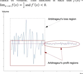
only exist when the transaction volume is low and the more volatile the transaction volume the more risky the arbitrage position. To see this, consider a stock with alternative large and low trading volume periods. In the large volume periods, any price move- ment can be interpreted as a change in the equilibrium price, worsening the mispricing, and the arbitrageur might not be able to bring back the price to his previous level: she will suffer a loss. In the low volume periods however, her trade will have an impact on the price and will hamper the price divergence: she will cash the liquidity premium. Finally, the closer these periods, the lower the probability to gain from the arbitrage position. Here again, in the worth case, the probability is 1/2.
We give in Fig. 1, an example of low and high volume periods. In the first part of the graph, we see that the risk to suffer a loss is high because of high volume volatility. In the second part of the graph, the arbitrageur’s strategy is always successful, and she faces no risk.
To generalize these remarks, we can suppose the existence of a function 𝑓 representing the link between qi and the
variance of volume. This function is such that 𝑓 0 = 1, lim!→!𝑓 𝑥 =!! and 𝑓! 𝑥 < 0.
Fig. 1. Volume volatility and profit and loss regions
On a stock-by-stock basis, the arbitrageur will choose to post the position on stock i that minimizes her risk on this stock. In our framework, the position to post on stock i minimizes the variance of volume, say 𝜎!!. To reduce her overall risk
however, the arbitrageur diversifies her positions, for a given expected gain. The individual variances of volume must be completed to take into account not only the risk on each stock, but also the joint risk on an arbitrage portfolio. The most natural way to do this is to take into account correlations between stocks volume. Large volume variations on one stock are a signal of a high liquidity risk. The arbitrageur’s allocation will depend on this volume volatility as well as correlations between volumes. The liquidity risk measure of an arbitrage portfolio can be extracted from the variance-covariance matrix of volumes Ω. The arbitrageur’s program allocates a volume Va on stock i
to satisfy the following constraints: 𝐶!: 𝑉!!≥ 0, for all 𝑖.
𝐶!: !𝑉!! 2𝑞!− 1 𝑐!= 𝐴.
𝐶!: 𝑉!! !
𝑃!∗− 𝑃! = 0.
The first constraint means that arbitrage is raising stock
trading volume. C2 corresponds to the expected gain of the
arbitrage portfolio, where the constant A gives the overall market illiquidity level. (2qi- 1) ciis the expected gain over
one unit of arbitrage on stock i. Finally, C3 ensures an overall
zero cost position to the arbitrageur. The arbitrageur problem is:
min!! 𝑉! !Ω𝑉!
𝑠. 𝑡. 𝐶!, 𝐶!, 𝐶! (7)
The resolution of this problem is very similar to the investor’s one in the CAPM context. The only difference comes from the risk matrix, w h i c h for the arbitrageur comes from the variability-covariability of volumes instead of returns in the classical framework of the CAPM. The efficient frontier is in the space illiquidity-risk. The form of the efficient frontier highly depends on the variance-covariance matrix of volumes.
As the investor’s problem, in the classical framework of the CAPM, can be solved in quantities or proportions, the arbitrageur problem can be written in volumes or turnovers. The use of turnovers allows to consider markets and stocks with very different overall number of shares. In this case, the key parameter is the variance-covariance matrix of turnovers and it is then not surprising to find this quantity in the very center of our model as it is in Lo and Wang (2000) approach. E. Numerical illustration
As an illustration of volume decomposition of any portfolio into its two components, we give a numerical example. In equilibrium, all agents should trade the market portfolio. However, due to market imperfections such as lack of liquidity on one side of the market, some of them will not hold a pure market - or index - portfolio. Consider an economy with three stocks - 1, 2 and 3 - and four agents - A, B, C and D where D is an arbitrageur. The characteristics of the stocks are summarized in the following table:
Stock OSNS Price Index Weight
1 40 1 0.50
2 20 1 0.25
3 20 1 0.25
where OSNS stands for the outstanding number of shares. Let agents A, B, C and D hold the following combinations of the three stocks:
A :[10 5 5] , B :[10 5 5], C :[20 10 1], D :[ 0 0 0]; saying that A and B hold 10 shares of stock 1 and 5 of stock 2 and 3 and agent C holds 20 shares of stock 1 and 10 of stocks 2 and 3, so that their investment in stocks 1, 2 and 3 in relative proportion is [0.5 0.25 0.25]. Hence, A, B and C hold pure benchmarked portfolios while agent D holds nothing.
Now suppose that due to some exogenous constraints, A, B and C decide to change their position. A wants to close her position, B to triple her risk exposure and C to lower hers by 50%. If they post their orders simultaneously to the market, B buys 20 shares of stock 1 (10 to A and 10 to C), 10 shares of stock 2 and 3 (5 to A and 5 to C). Their final positions are:
A :[0 0 0] , B :[30 15 15], C :[10 5 5];
In this situation, there is no tension on the market and the prices remain unchanged. Agents A, B and C’s trades can be summarized as:
A :[10 5 5] , B :[20 10 10], C :[10 5 5]. and there is no arbitrage since we get [20 10 10]
trades.
Consider now a situation where all the agents want to end up with the same positions as above, but if agent A still sell all her shares at once, agent B and C sequence their trades. Suppose that agent B trades first on stock 1 and 2 and postpones her trades on stock 3, while agent C trades on stock 2 and 3 and postpones her trades on stock 1.
A sells [10 5 5], B is willing to buy [20 10 0] and C is willing to sell [ 0 5 5]. If the matching is instanta-neous on stock 2, there is a lack of liquidity on the sell side for stock 1 (there are 20 shares to buy for only 10 to sell) and on the buy side for stock 3 (there are 10 shares to sell for not even one share to buy). These unbalances cause price pressures, w h i c h will raise the price of stock 1 and lower the price of stock 3. This price movement encourages agent D to enter the market to provide liquidity. Buying and selling the remaining quantities, she brings back the prices to their previous level until the equilibrium recovery. Doing so, he plays the role of a liquidity purveyor or a market maker.
Their positions between the two equilibriums are: A :[0 0 0], B :[30 15 5], C :[20 5 5], D :[ -10 0 10];
Agents A, B, C and D trades between the two equilibriums can be summarized as
A :[10 5 5], B :[20 10 10], C :[0 5 5], D :[ 10 0 10]; Once back to equilibrium, the arbitrageur will sell back the shares of stock 3 to agent B and buy the shares of stock 1 to agent C. The trading motives of agent C are to cash the liquidity premium, while agent B and C are adjusting their portfolio to end up with a pure market portfolio as in the case where there is no tension in the market. Hence, the agents trade [20 10 10] to move from the initial position to the intermediate position, and [10 0 10] once back at the equilibrium. The observed traded volume is [30 10 20] which represents [20 10 10] benchmark trades and [10 0 10] arbitrage trades. Note that the arbitrage represents in our example !"!!!!"
!"!!"!!"= 33% of the
activity observed in the volume. This example clearly shows that the reason for turnovers not to be equals comes from arbitrage.
III. EMPIRICAL DECOMPOSITION OF VOLUME
The previous section explains any positive deviation from the index turnover. In practice, the identification of arbitrage is straightforward. The idea is to isolate the lowest turnover among all stocks. The arbitrage is the excess in turnovers observed on the other stocks and the sum of all these extra turnovers is a measure of the overall illiquidity of the market. However, empirically, this is not a satisfactory measure as it depends only on one observation (the lowest turnover) and thus is not be robust. A better alternative is to work with averages by implicitly assuming that the overall illiquidity can be spread out over all stocks. The deviations from the
average turnover can now be either positive or negative, which fits better what we usually observed on markets. A. Motivation
Our approach comes from asset management practices, in which any portfolio can be decomposed into a market portfolio and an arbitrage portfolio. Applied to volume, we get a market component and an arbitrage component of the trading volume. The first factor in our volume factorial analysis can be identified as the market component whereas the remaining part will represent the arbitrage component. In our one-factor approach, stock turnovers inequality comes from the existence of arbitrage behaviors.
Consider a market where I assets, indexed by i = 1, . . . , I, are traded, by J market participants. The number of share outstanding for all assets is fixed and denoted by Ni.
Knowing the prices of all the assets at date t, we get the market value, say ∑kPktNk. The relative weight of asset i
compared to the market value is wit = PitNi / ∑kPktNk, where
Pit is the price of asset i at date t. This weight also stands for
its weight in the market portfolio. Consider that agent j portfolio differs from the market portfolio at date t. This portfolio depends on the weights αijt, i = 1, . . . , I, in all
assets. These weights can be decomposed in the following manner:
αijt=Iijt+Aijt (8)
i.e. the market component Iijt plus and arbitrage
component Aijt.The arbitrage component can either be
positive if asset I is over-weighted in agent j portfolio, or negative in the reverse case.
The same reasoning applies to trading volume for a particular asset. When an investor adjusts her portfolio, she buys or sells
a risky portfolio fairly close to the market portfolio. If her behavior is the one of an agent in equilibrium, she trades exactly the market portfolio. If her goal is to trade on her private information – concerning one asset or more – she will trade a quite different portfolio from the market portfolio. The extreme situation being agent j buying or selling only one asset. Therefore, the volume Vijt traded by agent j on
asset i at date t is the result of adjustments of both her index portfolio and her arbitrage portfolio. In terms of individual turnover, we can write:
𝑥!"# = 𝑥!"! + 𝑥!"!. (9)
Where 𝑥!"! stands for the index – or market – turnover and
𝑥!"! for the arbitrage turnover. Summing over all agents j, we
get an aggregate measure of the activity derived from risky positions adjustments on asset i, say:
𝑥!"! =!! !𝑥!"#! , (10)
and an aggregate measure of the activity derived from arbitrage strategies:
𝑥!"!=! ! 𝑥!"#
!
! , (11)
Note that the coefficient ½ corrects for the double counting when summing the shares over all investors.
Finally, at an aggregate level, we get for any asset, the following turnover decomposition:
𝑥!" =!
! !𝑥!"#= 𝑥!"
! + 𝑥
!"!. (12)
The practical interest of such decomposition is obvious and will be detailed in the following. On a theoretical point of view, the question is to identify the two components of the turnover from the observation of the sum.
Without any constraint, this identification cannot be done. For any agent i, the problem can be set up as the resolution of a one equation linear system with two variables; where the variables are the market portfolio and the arbitrage portfolio weights. This system has an infinite number of solutions and uniqueness can only be reached by imposing a constraint to the arbitrage portfolio.
B. Component identification
At an individual level, say for any agent j, the solution is straightforward and comes from portfolio management practices. A fund manager willing to invest in a pure arbitrage portfolio must have an identical risk exposure both on her long and short positions.
The risk exposure notion is not obvious but to make it simple, we assume that it can be captured by the invested value. Under this assumption, an arbitrage portfolio is thus said dollar neutral3 as opposed to beta-neutral portfolios where the fund manager adjusts the betas of the long and short positions. The constraint to impose in order to obtain a unique arbitrage portfolio is then obvious: any arbitrage portfolio must be dollar-neutral, and hence for all date t and agent j, it must satisfy:
𝑃!"
! 𝑁!𝑥!"#! = 0 (13)
From this constraint, we recover identification: if the portfolio is risk-neutral, then agent j uses the total value she trades at date t to adjust her market component. Knowing the market portfolio weights, and from the total number of shares traded by agent j, one can easily get her traded market portfolio. Deviations from this virtual portfolio give the arbitrage portfolio of agent j in traded volume. We get the decomposition in terms of turnover dividing the volumes by the number of shares outstanding.
At an aggregate level – when we only observe the total number of traded share, and without imposing any additional constraint, identification is not either possible. Here again we will follow the same reasoning. We suppose that the arbitrage activity satisfies a dollar neutral constraint saying that the value invested to buy is equal to the one received from selling. In all date t, the constraint is:
𝑃!"
! 𝑁!𝑥!"!= 0 (14)
and we get back the identification of the two components of the traded volume for stock i.
The decomposition between the benchmark portfolio and the arbitrage activity is as simple as in the individual case. The identification constraint imposes to the total traded value – or dollar volume – to be equal to the value traded on the market component in all date t. From the stocks weights in the market portfolio, we derive the number of shares traded for the benchmarked activity. The difference between this number of shares and the observed number of shares traded gives the level of the arbitrage activity.
IV. EMPIRICAL VALIDATION
In this section, we propose some empirical tests to discriminate between Lo and Wang (2000) interpretation of observed differences across stocks-turnover and ours. Conducting a principal component analysis on the stock turnovers can do this data reduction. Then the factors are analyzed and we carry on a simple empirical test to identify the first component to the market average turnover. Hence,
3The term dollar neutral refer to a zero-cost portfolio, i.e. a portfolio
any stock turnover, at all date, depends on an average term and a deviation term. The average part corresponds to trading volume coming from market portfolio adjustments. Our interpretation is that the deviation part is due to the opening and closure of arbitrage positions.
A second test consists in analyzing the dynamic properties of factors of order greater than one to discriminate between Lo and Wang (2000) interpretation and ours.
A. Principal component analysis and first factor identification
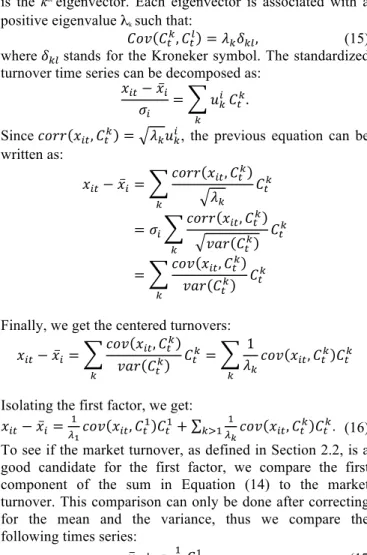
Let 𝑥!", i=1,…,T, t=1,…,T denote the turnover series. Since
the aim of principal component analysis is to explain the variance-covariance structure of the data through a few linear combinations of the original data, the first step is to calculate the I × I dimension variance-covariance matrix of the data. The spectral decomposition of this matrix leads to I orthogonal vectors, 𝐶!!= 𝑥!"!𝑢!, with dimension T, where uk
is the ktheigenvector. Each eigenvector is associated with a
positive eigenvalue λksuch that:
𝐶𝑜𝑣 𝐶!!, 𝐶!! = 𝜆!𝛿!", (15)
where 𝛿!" stands for the Kroneker symbol. The standardized
turnover time series can be decomposed as: 𝑥!"− 𝑥!
𝜎! = 𝑢!
! !
𝐶!!.
Since 𝑐𝑜𝑟𝑟 𝑥!", 𝐶!! = 𝜆!𝑢!!, the previous equation can be
written as: 𝑥!"− 𝑥!= 𝑐𝑜𝑟𝑟 𝑥!", 𝐶! ! 𝜆! ! 𝐶!! = 𝜎! 𝑐𝑜𝑟𝑟 𝑥!", 𝐶!! 𝑣𝑎𝑟 𝐶!! ! 𝐶!! = 𝑐𝑜𝑣 𝑥!", 𝐶! ! 𝑣𝑎𝑟 𝐶!! ! 𝐶!!
Finally, we get the centered turnovers: 𝑥!"− 𝑥!= 𝑐𝑜𝑣 𝑥!", 𝐶! ! 𝑣𝑎𝑟 𝐶!! ! 𝐶!! = 1 𝜆! ! 𝑐𝑜𝑣 𝑥!", 𝐶!! 𝐶 !!
Isolating the first factor, we get: 𝑥!"− 𝑥!= ! !!𝑐𝑜𝑣 𝑥!", 𝐶! ! 𝐶 !!+ !! ! !!! 𝑐𝑜𝑣 𝑥!", 𝐶!! 𝐶!!. (16)
To see if the market turnover, as defined in Section 2.2, is a good candidate for the first factor, we compare the first component of the sum in Equation (14) to the market turnover. This comparison can only be done after correcting for the mean and the variance, thus we compare the following times series:
𝑥!+ 𝜎! !
!!𝐶!
!, (17)
to the market turnover.
B. Dynamic properties of stock specific component
The empirical analysis of the dynamic properties of the factors, derived from the aforementioned approach, leads to an interpretation different from Lo and Wang (2000). In fact, any observed non-stationarity in the joint analysis of volume is due to the existence of non-stationary common factors. If the number of such factors is greater than one, the Lo and Wang type of analysis is the most accurate. On the contrary, if there is exactly one non-stationary factor, deviations from the first factor must be interpreted differently.
Whenever the first factor has been identified as the index – or benchmark – component of volume, we can focus on the analysis of the second component of the sum in Equation (16), and we get:
! !!
!!! 𝑐𝑜𝑣 𝑥!", 𝐶!! 𝐶!!. (18)
Once again, different interpretations are possible. Reference [24] sees this term as a hedging strategy against a risk associated with market conditions modifications. In this view, the first factor and the others are associated with investment decisions of the same kind. This implies that they should both present the same dynamic characteristics. On the contrary, we suppose that the second component is due
– or linked – to some short term arbitrage activity. Then the two components of the decomposition should feature very different dynamic behaviors. In particular, the first component should capture the entire trend observed in the turnover series whereas the second should be stationary. A standard stationarity test can then be a validation test of either one of the two approaches.
V. APPLICATIONS
In this section, we apply the approach presented above to daily data from the eight most important stocks from the FTSE index, namely AstraZeneca (AZN), Barclays Bank (BARC), GlaxoSmithKline (GSK), HSBC Holdings (HSBA), Lloyds TSB Group (LLOY), Royal Bank of Scotland Group (RBS), Shell Transport and trading co (SHELL) and Vodaphone Group (VOD) from May 17, 2000 to December 5, 2002. Note that, if intraday data seems to be a more appropriate choice when working on investment practices, the high intraday seasonality of volume and the associated intraday seasonal adjustment problems encourage us to work on daily data.
A. Data description
Table 1 gives some summary statistics about the eight aforementioned stocks from May 17, 2000 to December 5, 2002. Over this period and for all the stocks we have 648 trading days, i.e. 648 daily observations. Table 1 displays the mean, the standard deviation, the minimum and the maximum of the traded volume and the outstanding number of shares in millions of shares.
Over this period, volumes and outstanding number of shares are very different among stocks. In addition, stock ranking is roughly the same when considering daily averages of volume or number of shares outstanding. These observations justify the choice of turnovers instead of traded volumes.
A visual inspection of Fig. 2, which gives the evolution of volumes in daily number of traded shares, shows that some rises in volumes appear in all stocks, like at the end of September 2002 for example, whereas some other ones seem to be stock specific. These large jumps can even hide common rises of volume like for GSK, on November 30, 2001, where the daily traded volume reaches 193 200 000 shares compared to an average of 33 400 000 traded shares per day over the period.
This first analysis shows that the analysis of the traded volume must account for the total number of shares outstanding. Moreover, there seems to be two components in volume: a common component and a specific component. From these observations, we first propose a measure of volume corrected from the outstanding number of shares as
previously describe, that is the daily turnover in percentage. TABLE I
Descriptive statistics from Mai 17, 2000 to December 5, 2002.
Variables Traded volume Number of float shares
Statistics
Stocks Mean Std. Min/Max Mean Std Min/Max
AZN 5.1 3.0 0.27/28.6 1755 15 1730/1770 BARC 24.1 12.1 2.23/94.1 6508 265 5912/6628 GSK 14.2 10.4 1.15/193.2 5571 1077 3646/6218 HSBA 25.8 18.5 1.19/267.9 9269 222 8530/9431 LLOY 19.8 10.7 1.13/83.0 5528 31 5497/5561 RBS 9.2 7.3 0.55/141.4 2778 99 2586/2888 SHELL 33.4 19.2 3.19/133.9 9857 82 9733/9942 VOD 314.7 171.5 18.6/1458.8 65949 2696 61443/67895
Fig. 2. Daily traded volume evolution from May 17, 2000 and Dec. 5, 2002.
This measure is 100 times the daily traded volume divided by the float. Fig. 3 displays the evolution of the observed daily stock turnover ratio in percentage for the AZN from May 17, 2000 to December 20, 2002.
Because of this preliminary treatment, the volume series becomes comparable. The analysis of their dynamics shows the existence of a trend, whatever the stock. This trend appears also in the one-year daily average of stock turnover evolutions as shown in Table 2.
Fig. 3. Turnover evolutions from Mai 17, 2000 to Dec. 6, 2002, AZN.
TABLE II
One-year Daily turnover average evolutions from year 2000 to 2003.
Year Stocks 2000 2001 2002 AZN 0.226 0.260 0.368 BARC 0.364 0.327 0.422 GSK 0.208 0.233 0.302 HSBA 0.234 0.232 0.356 LLOY 0.288 0.321 0.440 RBS 0.288 0.312 0.383 SHELL 0.229 0.317 0.449 VOD 0.303 0.480 0.595
In fact, volume is rising at rates of about 16% to 96%. As this trend is observed on every stock, it should be captured by the common component of our decomposition. As a consequence, we will focus on the specific component of the decomposition and there is no need to correct from the initial series trend.
Our decomposition is a natural answer to this problem. We report summary statistics for the daily stock turnover ratio in percentage in Table 3.
The average turnover is quite different from one stock to another; the largest turnover being almost twice the lowest. However, this difference is mitigated by the use of turnover instead of traded volume series. In fact, the average traded volume for VOD (314 700 000 shares) was greater than 60 times the AZN average traded volume (5 100 000 shares). We can also note that the distributions of AZN, GSK, HSBA and RBS are the ones with the larger skewness and kurtosis and hence the most asymmetric with the largest tails.
B. Factor analysis
As seen before, the approach allows us to summarize the behavior of stock volume series over the entire period 2000-2002. The first factor explains 40.6 % of the variability-covariability of the stocks turnover. In the two following sections, the principal component analysis approach is conducted using daily data for the aforementioned stocks. However for presentation purposes, we report only the Figures for three stocks: GSK, AZN and RBS.
Fig. 4 reports the evolution of monthly averages of the first factor as well as the market turnover.
We cansee that the activity is quite stable during the year 2001. In October 2001, this activity sharply falls before recovering and starting to sharply increase during the rest of the period.
TABLE III
Descriptive statistics of stocks turnover.
Mean StD Skewness Kurtosis
AZN 0.29462 0.17424 2.91100 13.67123 BARC 0.37516 0.18373 1.80527 5.87145 GSK 0.25350 0.16400 9.08276 144.52370 HSBA 0.28050 0.20084 5.64628 55.75478 LLOY 0.35950 0.18862 1.82406 5.27974 RBS 0.33506 0.26048 9.74110 152.69574 SHELL 0.34444 0.19172 2.04292 6.15997 VOD 0.48319 0.24852 1.70851 5.58066
A visual inspection of the fit between the market turnover and the first factor confirms the identification of this factor to the benchmark - or index - component of volume.
Fig. 5 illustrates the nature of the second component that shows an erratic behavior around zero but no trend.
Fig. 4. Turnover (Market average turnover) and Index component (FI: dash line), monthly average evolution, May 2000-Dec. 2002.
To confirm these results, we calculate and report in Fig. 6, 7 and 8, the autocorrelation and the partial autocorrelation functions of the common and the specific components. If the index component is non-stationary and features long memory or changes in regime, the second component presents only short-term memory. Moreover, the individual analysis of the seven factors sum, i.e. the second component, shows that none of them is stationary. Hence, the non-stationarity is completely absorbed by the common component. This result fits the financial interpretation presented in Section 3. Moreover, the first component features the same seasonality as the turnover series. At an aggregate level, this also confirms that the two components cannot reflect the same type of portfolio management. The first component reflects long-term management strategies whereas the second component reflects short-term management strategies.
We conclude that the variability of stocks trading volume is well approximated by a two components model (a one factor model): an index component and an arbitrage component. C. Volume decomposition
In this section, we apply the principal component analysis to each stock separately and decompose each turnover – each volume measure - in a common and a specific components. The idea is to discriminate between investors’ interest for the market and a specific activity on the stock itself from the volume analysis. Over the entire period, and for all stocks, the activity is mostly driven by its index component.
Fig. 5. Evolution of the AZN specific component of volume, from May 17, 2000 to Dec. 6, 2002.
Fig. 6. Autocorrelation and partial autocorrelation functions of the two components, GSK Stock.
Fig. 7. Autocorrelation and partial autocorrelation functions of the two components, AZN Stock.
Fig. 8. Autocorrelation and partial autocorrelation functions of the two components, RBS Stock.
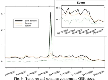
We see from Fig. 9 that the turnover evolutions follow the common component evolution up to the end of November 2001 and after the end of December 2001 for GSK. On the contrary, between these two dates, the specific component is driving the turnover evolution. This phenomenon is a direct
Fig. 9. Turnover and common component, GSK stock.
consequence of large fund management companies. In fact, these companies are sometimes modifying their holding in some groups in order to clear their position before the end of the year. These large transfers are usually done using applications4 at the end of the year. These trades, which do
4 An application is a buy-sell agreement concluded outside the
not correspond to any underlying market activity, are part of the traded volume. Fig. 9 illustrates such practices. Here, illiquidity is not the source of arbitrage. In such a case, we should replace the traded volume of November 29, 2001 by its index component to correct from this portfolio rebalancing clearing practice. This example is a practical application of our approach: it allows a data error correction method of the volume series when the errors come from particular financial practices.
From a general point of view, the AZN monthly average turnover evolution5 presents the same characteristics as the index turnover evolution [see Fig. 10]: a stability period in 2001 and an increase after December 2001. Moreover, from a visual inspection of the daily evolution of the AZN turnover and its component given in Fig. 10, we can assert that the activity is mostly driven by benchmarked strategies. However, the two series are not as close in July. This is due to the growing arbitrage activity at that time. As we can see, the arbitrage activity on AZN stock is growing from the very beginning of July and displays a peak on the July 17, 2002. This period corresponds to a pessimistic period concerning future profitability of AstraZeneca. In fact, AstraZeneca is a pharmaceutical company whose earnings come mostly from the production of one particular drug6. During that period, generics were promised access to the market very soon as the patent was expiring. This competition with their leading product was inducing a potential loss in AstraZeneca future earnings. This uncertainty was in favor of arbitrage strategies, which increased greatly at that time. This example is obviously rather a problem of information and uncertainty, which creates liquidity problems and not just a problem of liquidity. It shows that it is difficult to study separately liquidity and information, as information is an important source of liquidity variation.
Fig. 10. Turnover and common component, AZN stock.
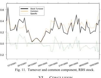
The last figure confirms the capacity of our statistical method to accurately extract seasonality as previously mentioned in Figures 6, 7 and 8. Fig. 11 shows the classical end of the year drop in volumes, which is completely captured in the common component and explains the RBS volume evolution between the December 24, 2001 and the very beginning of the year 2002.
5 This result is not shown here but is available upon request. 6 Their leading product represents 50 % of their earnings in 2001.
Fig. 11. Turnover and common component, RBS stock.
VI. CONCLUSION
In this paper, we propose a decomposition of trading volume using a factor analysis approach.
Using a simple theoretical model, we show that stocks’ volume, measured by turnover, can be decomposed just like returns. In fact, stocks’ turnover have a benchmark component as well as an arbitrage component that can be linked to arbitrage strategies and liquidity. The benchmark component of volume for a stock gives the interest of the market for this stock as being part of the market. The arbitrage component shows the interest of the market for this stock in particular.
The specific component of volume is a measure of stock trading volume corrected for trend, seasonal changes and data errors. This component can accurately help to better understand what is the information content of trading volume.
ACKNOWLEDGMENT
The authors gratefully acknowledge financial support of the chair QUANTVALLEY/Risk Foundation: Quantitative Management Initiative (QMI: www.QMInitiative.org). This research was supported by the project ECONOM&RISK (ANR 2010 blanc 1804 03).
REFERENCES
[1] T. Andersen, “Return Volatility and Trading Volume : An Information Flow Interpretation”, Journal of Finance, 51, 1996, 169-204.
[2] L. Bamber, “The Information Content of Annual
Earnings Releases: A Trading Volume Approach”, Journal of Accounting Research, 24, 1986, 40-56.
[3] L. Bamber, “Unexpected Earnings, Firm Size, and
Trading Volume Around Quarterly Earnings Announcements”, The Accounting Review, 1987, 510-532.
[4] J. Bialkowski, S. Darolles, and G. Le Fol, “Improving
VWAP strategies: A dynamic volume approach”, Journal of Banking and Finance, 2008, 32, 1709–1722.
[5] G.E.P. Box and G.C. Tiao, “A Canonical Analysis of a Multiple Analysis”, Biometrica, 70, 1977, 57-65.
[6] J. Campbell, S. Grossman, and J. Wang, “Trading
Volume and Serial Correlation in Stock Returns”, Quarterly of Journal of Economics, 108, 1993, 905-939.
[7] K.J.M. Cremers, J.and Mei, “Testing the Duo-factor
Model of Return and Volume”, unpublished.
[8] S. Darolles, G. Le Fol, and G. Mero, “When market
illiquidity generates volume”, unpublished.
[9] S. Darolles, G. Le Fol, and G. Mero, “Tracking
illiquidities in intradaily and daily characteristics”, unpublished.
[10] I. Domowitz, and J. Wang, “Auctions as algorithm :
computerized trade execution and price discovery”, Journal of Economic Dynamics and Control, 18, 1994, 29-60.
[11] D. Easley, and M. O’Hara, “Price, Trade Size, and
Information in Securities Markets”, Journal of Financial Economics, 19, 1987, 69-90.
[12] T. Epps, and T. Epps, “The Stochastic Dependence of
Security Price Changes and Transaction Volumes: Implications for the Mixture of Distribution Hypothesis”, Econometrica, 44, 1976, 305-321.
[13] F.D. Foster, and S.Viswanathan, “A Theory of Interday
Variations in Volumes, Variances and Trading Costs in Securities Markets”, Review of Financial Studies, 1990, 595-624.
[14] F.D. Foster, and S.Viswanathan, “Variations in Trading
Volume, Return Volatility and Trading Costs: Evidence on Recent Price Formation Models», Journal of Finance, 48, 1993, 187-211.
[15] R. Gallant, P. Rossi, and G. Tauchen, “Stock Prices and
Volume”, Review of Financial Studies, 5, 1992, 199-242.M. Young, The Technical Writer's Handbook. Mill Valley, CA: University Science, 1989.
[16] A.C. Harvey, “Forcasting structuring time series models
and the Kalman filter”, 1989, Book, (Cambridge University Press).
[17] J. Hasbrouck, and D.J. Seppi, “Common Factors in
Prices Order Flows and Liquidity”, Journal of Financial Economics, 59, 2001, 383-411.
[18] X. He, R. Velu, and C. Chen, “Commonality,
Information and Return/Return Volatility - Volume Relationship, unpublished.
[19] C. Heimstra, and J. Jones, “Testing for Linear and
Nonlinear Granger Causality in the Stock Price-Volume Relation”, Journal of Finance, 49, 1994, 1639-1664.
[20] J. Idier, C. Jardet, and G. Le Fol, “How liquid are
markets”, Bankers, Markets and Investors, 103, 2009, 150-58.
[21] J. Karpoff, “The Relation between Price Changes and
Trading Volume: A Survey”, Journal of Financial and Quantitative Analysis, 22, 1987, 109-126.
[22] J. Lakonishok, and S. Smidt, “Volume for Winners and
Losers: Taxation and Other Motives for Stock Trading”, Journal of Finance, 41, 1986, 951-974.
[23] B. LeBaron, “Persistence of the Dow Jones Index on
Rising Volume”, unpublished.
[24] A. Lo, and J. Wang, “Trading Volume: Definition, Data
Analysis, and Implication of Portfolio Theory”, The Review of Financial Studies, 13, 2000, 257-300.
[25] A. Lo, and J. Wang, “Trading Volume: Implications of
an Intertemporal Capital Pricing Model», Working Paper, MIT, 2001.
[26] J. Manchaldore, I. Palit, and O. Soloviev, “Wavelet
decomposition for intra-day volume dynamics”, Quantitative Finance, 2010, 10:8, 917-930.
[27] R. Merton, “An analytic derivation of the efficient
portfolio frontier”, Journal of Financial and Quantitative analysis, 7(4), 1972, 1851-1872.
[28] D. Morse, “Asymmetric Information in Securities
Markets and Trading Volume”, Journal of Financial and Quantitative Analysis, 15, 1980, 1129-1148.
[29] D. Pena, and G.E.P. Box, “Identifying a simplifying
structure in time series”, Journal of the American statistical Association, 82, 836-843.
[30] G. Richardson, S. Sefcik, and R. Thompson, “A Test of
Dividend Irrelevance Using Volume Reaction to a Change in Dividend Policy”, Journal of Financial Economics, 17, 1986, 313- 333.
[31] S. Ross, “Mutual Fund Separation in Financial Theory –
The Separating Distributions”, Journal of Economic Theory 17, 1978, 254-286.
[32] S. Smidt, “Long Run Trends in Equity Turnover”,
Journal of Portfolio Management, Fall, 1990, 66-73.
[33] A.R. Solow, “Detecting Change in the Composition of a
Multispecies Community”, Biometrics, 50, 1994, 556-565.
[34] S. Stickel, and R. Verrechia, “Evidence that Volume
Sustains Price Changes”, Financial Analysts Journal, 1994, 57-67.
[35] G. Tauchen, and M. Pitts, “The Price
Variability-Volume Relationship on Speculative Markets”, Econometrica, 51, 1983, 485-506.
[36] C. Ying, “Stock Market Prices and Volume of Sales”,
Econometrica, 34, 1966, 676-686.
Serge Darolles is Professor of Finance at université Paris-Dauphine where he has been teaching Financial Econometrics since 2012. Prior to joining Dauphine, he worked for Lyxor between 2000 and 2012, where he developed mathematical models for various investment strategies. He also held consultant roles at Caisse des Dépôts & Consignations, Banque Paribas and the French Atomic Energy Agency. Mr. Darolles specializes in financial econometrics and has written numerous articles which have been published in academic journals. He holds a Ph.D. in Applied Mathematics from the University of Toulouse and a postgraduate degree from EnSAE, Paris.
Gaëlle Le Fol is Professor of Finance at Paris–Dauphine and Research Fellow at the CREST (Centre de Recherche en Economie et Statistique). She is the scientific director of the QMI. She is an Economics and Econometrics graduate from the University of Paris 1 Panthéon – Sorbonne and holds a Ph.D. in Economics from Paris 1 University. Before joining the Université Paris-Dauphine, Gaëlle Le Fol was an Assistant Professor (Maîtres de Conférence) at the University of Paris 1 Panthéon – Sorbonne (1999-2002) and she became full Professor in Economics in 2002. Her research interests are in financial market microstructure and financial econometrics. Her recent research has included investors’ behaviors and their impact on the trading characteristics, market liquidity, contagion and systemic risk as well as high frequency algorithmic trading.