Self adhesion of semi-crystalline polymers between their glass transition temperature and their melting temperature

HAL Id: pastel-00001099

https://pastel.archives-ouvertes.fr/pastel-00001099

HAL is a multi-disciplinary open access

archive for the deposit and dissemination of sci-entific research documents, whether they are pub-lished or not. The documents may come from teaching and research institutions in France or abroad, or from public or private research centers.

L’archive ouverte pluridisciplinaire HAL, est destinée au dépôt et à la diffusion de documents scientifiques de niveau recherche, publiés ou non, émanant des établissements d’enseignement et de recherche français ou étrangers, des laboratoires publics ou privés.

Self adhesion of semi-crystalline polymers between their

glass transition temperature and their melting

temperature

Gauthier Jarrousse

To cite this version:

Gauthier Jarrousse. Self adhesion of semi-crystalline polymers between their glass transition temper-ature and their melting tempertemper-ature. Chemical Sciences. Université Pierre et Marie Curie - Paris VI, 2004. English. �pastel-00001099�

THÈSE DE DOCTORAT DE L’UNIVERSITÉ PARIS VI

Ecole Doctorale de Chimie Physique et Chimie Analytique

Spécialité :

Matière condensée : chimie et organisation

Présentée par :

Gauthier Jarrousse

pour obtenir le titre de :

DOCTEUR DE L’UNIVERSITÉ PARIS VI

Sujet de la thèse :

Adhésion des polymères semi-cristallins entre leur température

de transition vitreuse et leur température de fusion

Self adhesion of semi-crystalline polymers between their glass

transition temperature and their melting temperature

Soutenue le 13 Décembre 2004 devant le jury composé de :

Mme Liliane LEGER, Professeur, Collège de France Co-directrice de thèse M. Costantino CRETON, Directeur de recherche, ESPCI Directeur de thèse M. Jean-Claude WITTMANN, Directeur de recherche, Institut Charles Sadron Rapporteur M. Jean-Yves CAVAILLE, Professeur, INSA de Lyon Rapporteur M. Alain FRADET, Professeur, Université Paris VI Président M. John Christopher PLUMMER, Professeur, EPFL Invité

Table of contents

Introduction

Chapter 1 : Basic concepts and state of the art 4

1.1 Basic concepts

1.1.1 Brief introduction to polymers 1.1.1.1 Introduction

1.1.1.2 Types of polymers and classification 1.1.1.3 A few words on polymerization

1.1.1.4 Basic considerations of polymer physics 1.1.1.4.1 A single chain

1.1.1.4.2 Dense system of chains 1.1.1.4.3 The amorphous state

1.1.1.4.4 Mechanical properties of amorphous polymers 1.1.2 Semi-crystalline polymers

1.1.2.1 General structure of semi-crystalline polymers 1.1.2.2 Theories of crystallization kinetics

1.1.2.2.1 General considerations

1.1.2.2.2 Overall crystallization kinetics

1.1.2.2.3 Molecular mechanisms of crystallization 1.1.2.3 Melting

1.1.2.4 General mechanical behavior of semi-crystalline polymers 1.2 Fracture behavior of polymers

1.2.1 Introduction

1.2.2 Energy balance approach

1.2.3 The stress intensity factor approach

1.2.3.1 Plane strain, plane stress and different modes of fractures 1.2.3.2 Basic principles of the stress intensity factor approach 1.2.4 Relationship between G and K

1.2.5 Experimental considerations 1.3 Adhesion between polymers

1.3.1 Introduction

1.3.2 Different fracture mechanisms 1.3.2.1 Chain pullout

1.3.2.2 Chain scission 1.3.2.3 Crazing

1.3.2.4 Transition between the different mechanisms 1.3.3 Interdiffusion at polymer interfaces

1.3.3.1 Polymer interdiffusion

1.3.3.1.1 Diffusion at different time scales 1.3.3.1.2 Interdiffusion at polymeric interfaces

1.3.3.1.3 Fracture toughness and interdiffusion : early studies 1.3.4 Polymer adhesion between amorphous polymers : the modern view

1.3.4.1 Introduction

1.3.4.2 Direct adhesion between amorphous polymers

1.3.4.3 Reinforcement of interfaces (immiscible amorphous polymers) 1.3.5 Adhesion between semicrystalline polymers

1.3.5.1 Reinforcement of incompatible semicrystalline polymers 1.3.5.1.1 Compatibilization by formation of a copolymer

1.3.5.1.2 Compatibilizing less immiscible semicrystalline polymers 1.3.5.2 Self-adhesion of semicrystalline polymers

1.4 Conclusions and objectives of the current study

6 6 6 7 8 9 9 9 11 12 16 17 18 18 19 20 23 24 28 28 29 31 31 33 34 35 40 40 41 41 42 42 45 46 46 47 48 50 51 51 52 54 57 58 58 61 62 67

Chapter 2 : Characterizations and experimental techniques 68

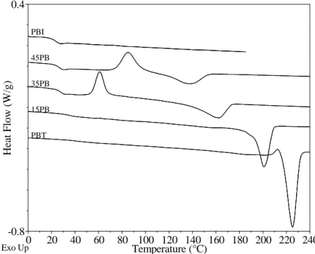
2.1 Brief review : structure and properties of PBT, PBI and PBT/PBI copolymers 2.1.1 PBT

2.1.1.1 Introduction 2.1.1.2 Crystallinity

2.1.1.3 WAXS study on PBT

2.1.1.4 The amorphous phase of PBT 2.1.1.5 Spherulitic structure

2.1.1.5.1 Lamellae 2.1.1.5.2 Spherulites

2.1.1.6 Crystallization and fusion 2.1.1.6.1 Crystallization 2.1.1.6.2 Cold crystallization 2.1.1.6.3 Fusion

2.1.1.6.4 Equilibrium melting temperature and heat of fusion 2.1.1.7 Some mechanical properties of PBT

2.1.2 PBI

2.1.3 PBT-PBI copolymers

2.2 Synthesis and molecular characterizations 2.2.1 Synthesis

2.2.2 End group analysis : determination of Mn

2.2.3 Rheology

2.2.4 NMR experiments 2.3 Bulk characterization

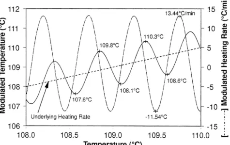
2.3.1 Temperature modulated Differential Scanning Calorimetry 2.3.1.1 Basic theory

2.3.1.2 Experimental procedure 2.3.2 Dynamic Mechanical Analysis

2.3.2.1 Experimental procedure 2.3.2.2 Results

2.3.3 X-rays

2.3.3.1 Sample preparation and results

2.3.3.2 Calculation of the degree of crystallinity 2.4 Adhesion : sample preparation and testing

2.4.1 Molding and assembling

2.4.1.1 Temperature controlled press 2.4.1.2 Molding

2.4.1.3 Cooling procedure 2.4.1.4 Assembling

2.4.2 Measurement of the fracture toughness 2.4.2.1 DCB tests

2.4.2.2 Measurements of the Young’s modulus 2.5 Tensile tests

2.5.1 Sample preparation 2.5.2 Tensile test

2.6 Study of the crystallinity at the interface

2.6.1 General procedure for optical and electron microscope observations 2.6.2 Optical observations

2.6.2.1 microtoming the sample

2.6.2.2 observation in polarized light microscopy 2.6.3 Observation in transmission electron microscopy

2.6.3.1 Sample preparation for TEM

2.6.3.2 transmission electron microscope observations

70 70 70 70 71 72 73 73 73 74 74 75 76 77 77 79 81 86 86 87 88 93 96 96 96 98 100 100 101 104 104 106 110 110 110 111 112 114 116 116 118 119 119 120 120 120 120 121 121 122 122 124

Chapter 3 : Results 126 3.1 PBT and 15PB 3.1.1 Adhesion measurements 3.1.2 DSC results 3.1.3 Microstructure 3.1.3.1 Optical observations 3.1.3.2 TEM observations

3.1.4 Simultaneous analysis of the different techniques 3.1.5 Partial conclusions 3.2 35PB and 45PB 3.2.1 Adhesion results 3.2.2 DSC results 3.2.3 Discussion 3.2.4 Conclusions 3.3 Amorphous 45PB : 45PBa

3.3.1 Characterization of the crystallinity of 45PBa by DSC 3.3.2 Crystallization kinetics

3.3.3 Observations of the samples 3.3.4 Tensile tests

3.3.5 Crystallinity and mechanical behavior 3.3.6 Adhesion results

3.3.7 Crack tip observations (optical and TEM) 3.3.8 Conclusions

3.4 PBI

3.4.1 Characterization of the crystallinity of PBI by DSC 3.4.2 Crystallization kinetics

3.4.3 Samples observations 3.4.4 tensile tests

3.4.5 Crystallinity and mechanical behavior 3.4.6 Adhesion results

3.4.7 Crack tip observation and TEM 3.4.8 Conclusion 129 119 131 135 135 138 140 142 144 144 146 152 154 156 157 168 172 175 176 177 184 187 188 188 193 195 198 199 200 205 209 Chapter 4 : Discussion 210

4.1 First set :contact between pre-crystallized samples 4.1.1 Overview of the results

4.1.2 Discussion on the mechanisms 4.1.3 Conclusions

4.2 Second set : quenched samples of 45PB and PBI 4.2.1 Overview of the results

4.2.2 Discussion on the mechanisms 4.2.3 Conclusions

4.3 Outlook and ideas for future studies

212 212 215 219 219 219 223 225 225 Conclusion 228 References 234

Adhesion is an immensely complicated subject concerned with the strength of the coupling that can occur between any pair of materials. It is also a subject of wide ranging usefulness with a steadily increasing importance in many technologies. The reason of the complexity of the science of adhesion lays in the fact that adhesion is at the cross section of many fundamental sciences, since in order to understand how two materials can be associated one should be aware of the different chemical or physical coupling that can occur at the interface.

In the present study, we consider only the adhesion between pairs of polymeric materials, and more specifically between semicrystalline polymers. This field has been widely but quite recently studied, since most of the polymers used in the industry are semicrystalline polymers. For example, the association of two or more polymers in alloys or in blends, to obtain optimized products by combining their properties, is of great industrial importance. Some of the industrial processes require a good and rapid adhesion such as the over molding process, where a polymer melt is injected on top of another polymer which is solid. In this type of process, the crystallinity at the very surface of the solid polymer is certainly playing a significant role and a better understanding of the way this crystallinity acts upon the adhesion is needed.

Although both the mechanisms of reinforcement of an interface between amorphous polymers and the fracture mechanisms of such interfaces are now relatively well established, their extension to semicrystalline interfaces is not straightforward. Several ideas have emerged from the studies of adhesion between semicrystalline polymers, but still a clear vision of the different mechanisms active for the reinforcement of the interfaces at the molecular level and the fractures mechanisms of such interfaces, is still far beyond reach.

The present investigation is a contribution aimed at elucidating the role of crystallinity upon adhesion and fracture mechanisms between semicrystalline polymers. Since the adhesion between amorphous polymers has been well described, the natural attempt in previous studies was to try to apply the mechanisms found in the case of amorphous polymers to the case of semicrystalline polymers. Although some similarities have been established, differences have been underlined such as the critical role played by the crystallinity.

Typically, it is well established that when co-crystallization occurs at the interface, the fracture toughness of such interfaces is largely increased. However, the conditions which will allow a co-crystallization are unclear. It has been shown also that the crystalline orientation at the interface had a great influence on the adhesion. However the reasons of this influence remain unknown.

Thus, several questions were at the onset of this work. What was the influence on the level of adhesion of the amorphous part of a semicrystalline polymer welded above Tg but

below Tm. Was there a degree of crystallinity below which the amorphous part is the

principal actor of the adhesion?

Other questions emerged quite rapidly after starting this work. What could be the preponderant mechanism of interface reinforcement (co-crystallization, interdiffusion, crystalline reorganization at the interface)? Was it possible to enhance the adhesion by cold crystallizing samples in contact? What was the influence of the crystalline structure at the interface on adhesion?

In order to try to answer these questions, we coupled several experimental techniques providing information on the crystallinity in the bulk (Temperature Modulated Differential Scanning Calorimetry), and at the interface (optical and TEM observations), as well as on the degree of adhesion (double cantilever beam test).

We decided to work with a model system of copolymers, all synthesized by step-growth polymerization with nearly identical average molecular weights and molecular weight distributions, and with nearly identical Tg, but with an overall crystallinity which could be

varied (by using copolymers with different overall degrees of crystallinity and different crystallization kinetics). This system was much more complicated than initially thought, since the overall degree of crystallinity was indeed not the only parameter which varied between the different copolymers. However, by a detailed characterization of this complex system, it was possible to investigate the different effects of the crystallization behavior on adhesion.

A key experimental aspect of our work was the careful control of temperatures and temperature gradients. All of our copolymers are very sensitive to thermal history because of the inherently slow nature of the crystallization process in polymers. In turn the crystallization process affected both adhesive and mechanical properties of the polymer, which is a fact reflected in the values of fracture toughness that we measured by DCB. We specially built a mold to realize bilayers with a precise control of the temperature of each surface and of the interface. Cooling conditions were well controlled to be reproducible and to span a wide range of cooling rates.

With these tools in hand, our goal was to realize a comprehensive and thorough investigation of adhesive mechanisms potentially active below the melting point of the crystalline phase of semi-crystalline polymers. After a chapter introducing the main concepts used in the analysis of the experimental work and a review of the state of the art, chapter 2 is dedicated to the characterization of the materials and the bulk of the results are presented in chapter 3. Chapter 4 summarizes the main results and discusses them in a more general view also in relation with previous work on the topic and finally the conclusion summarizes the main results.

Chapter 1

Introduction to the adhesion of semicrystalline polymers and state of

the art

Table of contents

1.1 Basic concepts

1.1.1 Brief introduction to polymers 1.1.1.1 Introduction

1.1.1.2 Types of polymers and classification 1.1.1.3 A few words on polymerization

1.1.1.4 Basic considerations of polymer physics 1.1.1.4.1 A single chain

1.1.1.4.2 Dense system of chains 1.1.1.4.3 The amorphous state

1.1.1.4.4 Mechanical properties of amorphous polymers 1.1.2 Semi-crystalline polymers

1.1.2.1 General structure of semi-crystalline polymers 1.1.2.2 Theories of crystallization kinetics

1.1.2.2.1 General considerations

1.1.2.2.2 Overall crystallization kinetics

1.1.2.2.3 Molecular mechanisms of crystallization 1.1.2.3 Melting

1.1.2.4 General mechanical behavior of semi-crystalline polymers 1.2 Fracture behavior of polymers

1.2.1 Introduction

1.2.2 Energy balance approach

1.2.3 The stress intensity factor approach

1.2.3.1 Plane strain, plane stress and different modes of fractures 1.2.3.2 Basic principles of the stress intensity factor approach 1.2.4 Relationship between G and K

1.2.5 Experimental considerations 1.3 Adhesion between polymers

1.3.1 Introduction

1.3.2 Different fracture mechanisms 1.3.2.1 Chain pullout

1.3.2.2 Chain scission 1.3.2.3 Crazing

1.3.2.4 Transition between the different mechanisms 1.3.3 Interdiffusion at polymer interfaces

1.3.3.1 Polymer interdiffusion

1.3.3.1.1 Diffusion at different time scales 1.3.3.1.2 Interdiffusion at polymeric interfaces

1.3.3.1.3 Fracture toughness and interdiffusion : early studies 1.3.4 Polymer adhesion between amorphous polymers : the modern view

1.3.4.1 Introduction

1.3.4.2 Direct adhesion between amorphous polymers

1.3.4.3 Reinforcement of interfaces (immiscible amorphous polymers) 1.3.5 Adhesion between semicrystalline polymers

1.3.5.1 Reinforcement of incompatible semicrystalline polymers 1.3.5.1.1 Compatibilization by formation of a copolymer

1.3.5.1.2 Compatibilizing less immiscible semicrystalline polymers 1.3.5.2 Self-adhesion of semicrystalline polymers

1.4 Conclusions and objectives of the current study

6 6 6 7 8 9 9 9 11 12 16 17 18 18 19 20 23 24 28 28 29 31 31 33 34 35 40 40 41 41 42 42 45 46 46 47 48 50 51 51 52 54 57 58 58 61 62 67

This chapter has the dual purpose to briefly present the basic concepts of polymer science and fracture mechanics needed to understand my experimental work as well as to review the state of the art in the adhesion between two identical semicrystalline polymers.

We will start with some basic concepts of polymer science which are meant to be a short introduction to the semicrystalline polymers section, in which more details will be given.

Knowing those basic notions on amorphous and semicrystalline polymers, we will introduce some well known concepts in the fracture behavior of polymers, concepts that will be applied in polymer adhesion problems.

Finally, a comprehensive state of art of the field of adhesion between polymers will then be presented, first with examples of adhesion between amorphous polymers and then between semicrystalline polymers.

1.1 Basic concepts

In this section, we will present basic notions on polymers. We will focus on the notions required for the characterization of the materials used in this study and for the interpretation of our adhesion results.

1.1.1 Brief introduction to polymers

A very brief introduction will be given in this section. A more detailed introduction to polymer science can be found in the textbooks of Young and Lovell1 and Strobl2.

1.1.1.1

Introduction

The notion of macromolecule appears in 1922 in the studies of Staudinger, and can be defined as follows : a macromolecule is a long molecule containing atoms held together by primary covalent bonds along the molecule.

Macromolecules are made by a process called polymerization whereby monomer molecules react together chemically to form linear or branched chains or three-dimensional networks.

1_{Young, R. J. and Lovell, P. A. Introduction to polymers. (Chapman & Hall, London, 1991} 2_{Strobl, G. The Physics of Polymers. (Springer-Verlag, Berlin, 1996)}

A macromolecule is characterized by its molar mass M related to the degree of polymerization x, which is the number of repeat units in the macromolecule, by the simple relation :

0

M

=

xM

where M0 is the molar mass of the repeat unit.

The term polymer is applied when the number of repeat units is typically above one hundred. Experimentally, for such a number of repeat units, properties such as the melting temperature, become x-independent.

Experimentally the synthesis of macromolecules leads to polymers which consist of chains with a range of molar masses, which changes discontinuously in intervals of M0. It

is convenient to characterize the distribution in terms of mass averages. Considering Ni

macromolecules of mass Mi, the number-average mass, Mn and the weight-average mass,

Mw are defined as follows (equation 1.1-2 and 1.1-3) :

The ratio I = Mw/Mn represents the polydispersity of the material and is an indication of

the breadth of the molecular weight distribution.

1.1.1.2

Types of polymers and classification

We can classify the different polymers as follow : Thermoplastics, which can melt upon the application of heat, elastomers which are crosslinked rubbery polymers that can be stretched easily to high extensions and which rapidly recover their original dimensions and thermosets which normally are rigid materials and are network polymers in which chain motion is greatly restricted. Elastomers and thermosets are intractable once formed and degrade rather than melt upon the application of heat.

Thermoplastics are widely used in industry because they can be molded into virtually any shape using processing techniques. Generally, thermoplastics do not crystallize easily upon cooling to the solid state because crystallization requires considerable ordering of the highly coiled and entangled macromolecules. Those which do crystallize are rather semi-crystalline with both crystalline and amorphous regions. Amorphous polymers are

i i i n i i

N M

M

N

=

∑

∑

N M

M

N M

=

∑

∑

characterized by their glass transition temperature Tg while semi-crystalline polymers are

characterized by both the glass transition and the melting temperature Tm.

If only one type of monomer is used the resulting polymer is called a homopolymer whereas if more than one type of monomer is used the polymer is termed a copolymer.

There are several categories of copolymers, each being characterized by a particular form of arrangement of the repeat units along the polymer chain. If two types of monomer are used, we can classify the copolymers as follows :

- Statistical copolymers are copolymers in which the sequential distribution of the repeat units obeys known statistical laws. Random copolymers are statistical copolymers in which the distribution is truly random.

- Alternating copolymers are arranged in a strictly alternating way along the polymer chain.

Block copolymers are linear copolymers in which the repeat units exist only in long sequences, or blocks, of the same type.

- Graft copolymers are branched polymers in which the branches have a chemical structure different from that of the main chain

Statistical copolymers -A-A-B-A-B-B-B-A-A-B-B-A-A-A-A-B-A-A-B-B-B-A- Alternating copolymers -A-B-A-B-A-B-A-B-A-B-A-B-A-B-A-B-A-B-A-B-A-B- Block copolymers -A-A-A-A-A-A-A-A-A-A-A-B-B-B-B-B-B-B-B-B-B-B-

Graft copolymers -A-A-A-A-A-A-A-A-A-A-A-A-A-A-A-A-A-A-A-A-A-

1.1.1.3

A few words on polymerization

The synthesis of polymers is a very large and extensive topic. It is covered in details in several textbooks (Rempp and Merrill1, Champetier and Monnerie2 and Odian3). Synthesis of polymers can be divided into two main categories, namely step-growth polymerizations, where the polymer chains grow step-wise by reactions that can occur between any two molecular species, and chain growth polymerization, where a polymer chain grows only by reaction of individual monomers with a reactive end-group on the growing chain.

We will focus here on polycondensations, which are step polymerizations that involve reactions in which small molecules are eliminated.

1_{Rempp, P. and Merrill, E. W. Polymer Synthesis. (Hüthig & Wepf Verlag Basel, New York, 1991)} 2 _{Champetier, G. and Monnerie, L. Introduction à la chimie macromoléculaire. (Masson, Paris, 1969)} 3 _{Odian, G. Principles of Polymerization. (Wiley, New York, 1981)}

B-B-B-B-B-B-B

The formation of polyesters is typical of these reactions and may be represented more generally by :

n HOOC-R1-COOH + nHO-R2-OH ÆH-[-OOC-R1-COO-R2-]n-OH + (2n-1)H2O

1.1.1.4

Basic considerations of polymer physics

From section 1.1.1.1, we saw that the polymer was constituted of macromolecules made of hundreds of repeat units. In order to understand the basic properties of polymers, it is useful to consider its constituent, the chain, from a physical point of view (de Gennes1).

1.1.1.4.1

A single chain

One of the simplest idealizations of a flexible polymer chain consists in replacing it by a random walk on a periodic lattice. The succession of N steps will lead to the following mean square end to end distance

It has been also demonstrated that the radius of gyration of a Gaussian chain has the same dependence with N, i.e. :

1.1.1.4.2

Dense system of chains

From a static point of view, the chains in a polymer melt can be considered as Gaussian and ideal (Flory2).

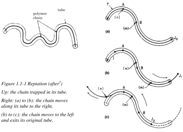
The dynamics of a chain among others has been well described by the so-called reptation model proposed by de Gennes3 and Doi and Edwards4.

In a melt, the chains can move by Brownian motion, but they cannot intersect each other. A useful picture is to consider the chain trapped in a network. The chain is not allowed to cross any obstacle but can move in between in a wormlike fashion, called reptation. Edwards introduced the notion of tube, which contains the chain as represented in Figure 1.1-1.

1_{de Gennes, P. G. Scaling concepts in Polymer Physics (Cornell university press, London, 1979)} 2_{Flory, P. J. Journal of Chemical Physics, 17: 303, (1949).}

3_{de Gennes, P. G. Journal of Chemical Physics, 55: 572-579, (1971).} 4

Doi, M. and Edwards, S. J. Journal of the Chemical Society; Faraday Transactions 2, 74: 1789-1801, 1802-1818, 1818-1832, (1978). 2 2

r

=

Na

~

R

N

a

Figure 1.1-1 Reptation (after3) Up: the chain trapped in its tube. Right: (a) to (b): the chain moves along its tube to the right,

(b) to (c): the chain moves to the left and exits its original tube.

1

de Gennes

The diameter of the tube is given by d~Ne 1/2

a, a being the monomer length and Ne the

average number of monomers between entanglement points, i.e. between the topogical obstacles.

The tube diffusion coefficient, Dtube, is given by the Einstein relationship kT/f where the

friction coefficient f is 6πη1Na :

where η1 is a local the viscosity of the polymer melt.

During the reptation time τrept, the chain moves over Ltube along the tube and over Rtube in

the real space :

so :

1

de Gennes, P. G. Scaling Concepts in Polymer Physics. (Cornell University Press, London, 1979)

1

6

kT

D

Na

πη

=

tube rept tube e

e e

N

N

D

L

d

N a

N

N

τ

=

=

⎛

_⎜

⎞

_⎟

=

⎛

_⎜

⎞

_⎟

⎝

⎠

⎝

⎠

self rept tube e

N

D

R

d

Na

N

τ

=

=

=

_{Eq. 1.1-8}

In the case of a polymer with Ne~100 and N~10 000 we get a reptation time of the order

of magnitude of 1 sec and a self diffusion coefficient of 10-11 cm2.sec-1.

These are the basic equations of the diffusion of a polymer chain in a melt, which will be used later on in the description of interdiffusion at polymeric interfaces.

1.1.1.4.3

The amorphous state

If the melt of a non-crystallizable polymer is cooled, it becomes more viscous and flows less readily. If the temperature is reduced low enough it becomes a transient (“rubbery”) network of entanglements and then as the temperature is reduced further, the sample becomes a relatively hard elastic polymer glass. The temperature at which the polymer undergoes the transformation from a transient network to a glass is known as the glass transition temperature, Tg. The ability to form glasses is not confined to

non-crystallizable polymers. Any material which can be cooled sufficiently fast to avoid crystallization will undergo a glass transition.

Amorphous polymers can be thought of as frozen polymer liquids, in which no well defined order can be found.

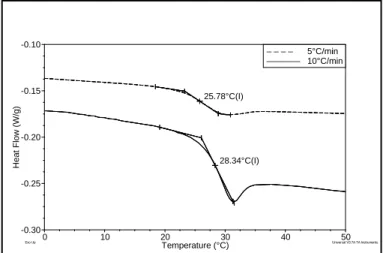
The glass transition temperature can be detected experimentally by the variation of the specific volume as represented in Figure 1.1-2 or, as carried out in our study, by differential scanning calorimetry (DSC) (Figure 1.1-3).

3 3 1

6

a N

kT

N

πη

τ

=

6

N

kT

D

a N

πη

=

1

We may consider the amorphous state as an isotropic and out of equilibrium state. More extensive treatments of the amorphous state can be found in textbooks : Gedde1

1.1.1.4.4

Mechanical properties of amorphous polymers

Polymers exhibit a wide range of elastic properties depending upon their structure and testing conditions. Figure 1.1-4 shows the variation of Young’s modulus, E, with temperature for an amorphous polymer. At low temperature, the polymer is glassy with a relatively high modulus of the order of a few GPa. Above Tg, the polymer becomes

1

Kovacs, A. J. Journal of Polymer Science, 30(121): 131-147, (1958).

Figure 1.1-2 : variation of the specific volume of poly(vinyl acetate) with temperature taken after two different times (After Kovacs1)

25.78°C(I) 28.34°C(I) -0.30 -0.25 -0.20 -0.15 -0.10 H eat F low (W /g) 0 10 20 30 40 50 Temperature (°C) – – – – 5°C/min ––––––– 10°C/min

Exo Up Universal V3.7A TA Instruments

Figure 1.1-3 : variation of the heat flow of poly(butylene terephthalate-co-butylene isophthalate) with the heating ramp

viscoelastic with a lower modulus, very rate and temperature dependent. For polymers with relatively high molecular weight, typically higher than the average molecular weight between entanglements, Me, the polymer can be considered as a transient network, with a

modulus remaining approximately constant with increasing temperature. With a very simple molecular theory of rubber elasticity, it can be shown that the shear modulus, G, of a transient network is given by an equation of the form :

where ρ is the density of the polymer and T the temperature at which the modulus is calculated (ν the Poisson’s ratio is typically equal to 0.5 for most polymers above their transition temperature). This expression is remarkably accurate given the assumptions contained in the model.

The mechanical behavior of polymers depends upon the testing rate as well as the temperature and it is found that there is a general equivalence between time or frequency of observation and temperature. The mechanical response can be represented in a procedure known as time-temperature superposition. In a series of mechanical measurements made over a range of temperatures at different testing frequencies, the data can be put onto a simple ‘master curve’ by shifting the data measured at one temperature along the frequency axis by a factor which is a function only of the test temperature, as represented in Figure 1.1-5. This is a very general property of many polymers and is due to the fact that the spectrum of relaxation times of a polymer has typically the same temperature dependence.

In a range of temperatures between Tg and Tg + 100°C, the relationship between the test

temperature and this factor aT is often given by an equation of the form

1_{Gedde, U. W. Polymer Physics. (Kluwer Academic Publisher, 1995)}

2(1

)

E

RT

G

M

ρ

ν

=

=

+

Figure 1.1-4: variation of E for an amorphous polymer

where C1 and C2 are constants and Tref is a reference temperature. This equation is

normally termed the WLF (Williams-Landel-Ferry) equation and is based on the notion that molecular mobility depends on the available free volume which vanishes for a finite temperature T∞.

Figure 1.1-5 : Building a master-curve with the time-temperature superposition. A typical feature of the mechanical behavior of polymers is the way in which their mechanical response to an applied stress or strain depends upon the rate or time period of loading. This behavior can be thought of as being somewhere between that of elastic solids and liquids. The subject of viscoelasticity is covered in several textbooks (Ferry, Ward, Young and Lovell) and so only a very brief review will be given here.

An example of viscoelastic behavior is given in Figures 1.1-6 and 1.1-7 in two particular experimental cases : creep and relaxation.

When a sudden stress is applied to a polymeric sample and maintained, the measured deformation increases with time: This property is called creep and it is an indication of the viscoelastic character of the material, as shown on Figure 1.1-6. When a sudden deformation is applied to a polymeric sample and maintained, the measured force decreases as a function of time: This is called stress relaxation and is illustrated on Figure 1.1-7.

(

)

(

)

log

C T

T

a

C

T

T

−

−

=

+

−

σ0 t σ t ε viscous elastic viscoelastic ε0 t ε σ t viscous elastic viscoelastic Figure 1.1-6 : Creep of a viscoelastic material at a constant applied stress.

Figure 1.1-7 : Relaxation of a viscoelastic sample submitted to a constant strain.

The viscoelastic behavior of polymers is often examined using a dynamic mechanical testing where the polymer is subjected to an oscillating sinusoidal stress. Unlike an elastic material, the strain lags somewhat behind the stress and so the variation of stress and strain with time can be given by expressions of the type

where ε0 and σ0 are the strain and stress amplitude, ω is the frequency and δ the phase

angle or phase lag. This approach leads to the definition of two dynamic moduli, G’ which is in-phase with the strain and represents the elastic part of the modulus and G’’ which is π/2 out-of-phase with the strain and represents the viscous part of the modulus. G’ and G’’ or E’ and E’’ in uniaxial tension, are sometimes called the storage component and the loss component of the complex modulus respectively. It follows that the loss factor tanδ is given by

and a ‘complex modulus G* can be defined as :

The value of tanδ like the value of the complex modulus varies with temperature, and peaks are observed at certain temperatures, as shown in the example given in Figure 1.1-8. These peaks of dissipation are attributed to dissipative molecular motions and called transitions. In an amorphous polymer, the most pronounced peak is the α-transition which

( )

ε ε

ω

(

)

σ σ

ω δ

tan

G

G

δ

=

G

=

G

+

iG

corresponds to the onset of molecular motion at the Tg and the β and γ relaxations are due

to localized main-chain or side group motion. For semi-crystalline polymers, the interpretation of the transitions can be less obvious but usually a Tg can still be detected in

this way.

1

1.1.2 Semi-crystalline polymers

Some polymers, when cooled from the melt, have the ability to form ordered domains, before going through the glass transition temperature below which the motions are drastically reduced, forbidding any more ordering.

A polymer will never be fully ordered, in other words a polymer will never be fully crystallized, from cooling it from melt. In an entangled system of chains, forming ordered regions will largely reduce the entropy. Because of entanglements, a polymer will not fully crystallize within a reasonable time. A mix of ordered and disordered regions will be obtained. Thus, the polymers can be described as semicrystalline, since polymers crystallized in the bulk state are never totally crystalline and have both crystalline and amorphous regions.

Both thermodynamics and kinetics govern the crystallization of polymers. For thermodynamics, it is useful to consider the Gibbs free energy of any system related to the enthalpy H and the entropy S (equation 1.1-17).

G=H−TS Eq. 1.1-17

Figure 1.1-8 : variation of tanδ with temperature for amorphous polystyrene (after McCrum et al.1)

The system is in equilibrium when G is a minimum. Below the melting temperature Tm,

crystallization may occur as the corresponding large reduction in enthalpy ∆Hm will be

greater than that of the product of the melting temperature by the entropy change (Tm∆Sm).

Crystallization is also controlled by kinetics, as it is possible to obtain a crystallizable polymer in the amorphous state by a rapid cooling from the melt.

The kinetics of crystallization will be discussed in the following sections after a general presentation of the structure of semicrystalline polymers.

We must underline the fact that molecular mobility is needed to achieve ordered regions, thus the melting temperature, Tm, of a semicrystalline polymer will always be above its

glass transition temperature.

The crystallization of polymers is of enormous technological importance, as many thermoplastics polymers used in the industry will crystallize when the molten polymer is cooled below the melting point of the crystalline phase. The presence of crystals has an important effect upon the polymer properties and indeed on adhesion which is the topic of our study.

We will now concentrate on melt-crystallized polymers. Some general reading on the crystalline state in polymers can be found in the following references : Sperling2, Tadokoro3, Wunderlich4, Young and Lovell5.

1.1.2.1

General structure of semi-crystalline polymers

Crystalline solids consist of regular three-dimensional arrays of atoms placed at the node of a repeating unit known as the unit cell. In polymers, the mers are placed at those nodes, imposing to the chains to pack together side by side, with their main axis along one of the sides of the unit cell. Usually, the chains are considered to lie along the c-axis of the unit cell.

The structure of a semicrystalline polymer is composed of crystalline domains separated by regions of amorphous polymer. The crystalline morphology is complex and has several levels of structure, as shown schematically in Figure 1.1-9.

1_{McCrum, et al. Anelastic and dielectric effets in polymeric solids. (John Wiley, London, 1967)} 2 _{Sperling, L. H. Introduction to physical polymer science. (Wiley-interscience, New York, 1992)} 3 _{Tadokoro, H. Structure of Crystalline Polymers. (Wiley-Interscience, New York, 1979)} 4

Wunderlich, B. Macromolecular Physics. (Academic Press, Orlando, 1973)

The smallest level is the unit cell which can be assigned to one of the seven basic crystal systems (triclinic, monoclinic, etc.). The polymer molecule is generally lying parallel to the c axis although there are exceptions. The crystalline domains form then lamellae that grow out from a central nucleation point. The polymer chain which is much longer than the typical thickness of the lamella (from 5 to 50 nm roughly) must reenter several times in the lamella. There are mainly two models that describe the reentry : the folded chain model and the switchboard model. In the first model, the chain folds back and forth with hairpin turns, leading to an adjacent reentry, while in the second model the reentry is more random like an old-time telephone switchboard. In Figure 1.1-9 the second model is represented since, in the case of melt-crystallized polymer, this type of reentry is more likely to occur. The lamellae form a superstructure called spherulite. Under polarized light, this superstructure of typically 5 to 500 µm in diameter, shows the characteristic Maltese cross, as represented in figure 1.1-9.

1.1.2.2

Theories of crystallization kinetics

1.1.2.2.1

General considerations

When the temperature of a polymer melt is reduced below the melting temperature there is a tendency for the random entangled molecules in the melt to become aligned and form small ordered regions. This process is known as nucleation and the ordered regions are called nuclei. The second step in the crystallization process is growth whereby the crystal nucleus grows by the addition of further chains.

Crystallization is therefore a two step process, nucleation and growth, which can be imaged by raindrops falling in a puddle. These produce expanding circles of waves that

l

a

c

b

intersect and cover the whole surface. The expanding circles of waves, of course, are the growth fronts of the spherulites and the points of impact are the crystallite nuclei.

In the majority of cases of crystallization from polymer melts, nucleation takes place heterogeneously. The number of nuclei depends upon the temperature of crystallization and upon the presence of foreign bodies or interfaces. The growth of a crystal nucleus can take place in either one, two or three dimensions.

When the radial growth rate is plotted as a function of crystallization temperature, a maximum is observed, due to the competition between the thermodynamic driving force for crystallization, which increases as the temperature is lowered, and the viscosity, which will act against the transport of material to the growth point.

1.1.2.2.2

Overall crystallization kinetics : Avrami’s equation

A polymer melt of volume VL is cooled below the crystallization temperature. If we

assume that the nucleation is homogeneous, the number of nuclei formed at a given temperature per unit time per unit volume N is constant. In the time interval dt, NVLdt

nuclei are formed. After a length of time t, these nuclei become spherulites with a volume of (4/3)πr3 or (4/3)πg3t3 with r = gt (g is known as the growth rate). The total volume of spherulitic material, VS, present at time t, and grown from the nuclei formed in the time

interval, dt, is ruled by the differential equation :

The crystallized fraction is given by X = VS/VL and making the assumption that volume of

the crystalline phase is small compared to VL, we have dX=dVs/VL.

dX should be corrected by a factor (1-VS/VL) due to the meeting of the developing entities

and to the reduction of the volume of liquid. We finally get :

and upon integration

Equation 1.1-20 is only valid in the initial stages of crystallization (VL>>VS). If types of

nucleation and growth other than those considered here are found, equation 1.1-20 can be expressed as 3 3

4

3

dV

=

π

g t NV dt

( )

4

1

( )

3

dV

dX t

g Nt

X t

V

π

=

=

−

π

which is the Avrami1’s equation. The exponent n is called the Avrami’s exponent. Experimentally, it is useful to express the Avrami’s equation with the difference in height of a liquid in a dilatometer :

V0, h0 and V∝, h∝ are the initial and final volume and height respectively, Vt, ht the volume

and height at time t.

1.1.2.2.3

Molecular mechanisms of crystallization

Although Avrami’s equation provides a useful guide for the overall kinetics of crystallization, it does not give any insight into the molecular process involved in the nucleation and growth of polymer crystals.

The most widely accepted approach at a molecular level, is the kinetic description of Hoffman et al.2. It is essentially an extension of the approach used to explain the kinetics of crystallization of small molecules.

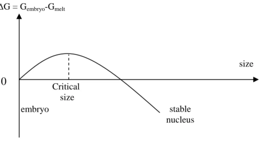
Let us consider again the Gibbs equation (equation 1.1-17). In the primary step of crystallization, i.e. nucleation, a few molecules pack together to form a crystalline embryo. This process will change the Gibbs free energy : the creation of a crystal surface will tend to cause G to increase while the incorporation of molecules in the crystal causes a reduction of G. A schematic representation of the change in free energy is given in Figure 1.1-10.

1_{Avrami, M. Journal of Chemical Physics, 7: 1103, (1939).} 2

Hoffman, J. D et al. Treatise on Solid State Chemistry. (Plenum, New York, 1976)

(

)

1

−

X t

( )

=

exp

−

Zt

(

)

The peak in the curve may be regarded as an energy barrier, which could be overcome by sufficient thermal fluctuation at the crystallization temperature. Once the nucleus is greater than the critical size it will grow spontaneously as this will cause G to decrease.

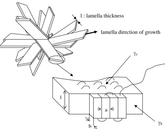
In Hoffman’s approach, the polymer crystal is considered to grow on a preexisting crystal surface. We will take as an example the growing on the surface of a lamella (Figure 1.1-11). In this process, new chain segments are added by chain folding on the smooth crystal surface. Assuming that the lamella has a fold surface energy γe and a lateral surface

energy γS, the change in free energy in the lamella involved in laying down n adjacent

molecular strands or stems of length l will be

the first part 2blγS+2nabγe being the increase of free energy due to the increase in surface

and nabl∆Gv being the reduction in free energy because of the incorporation of stems in

the crystal.

At the “equilibrium melting temperature” T0m, we have

so, by introducing the degree of under cooling ∆T = (T0m-T), we get

For a large number of stems n, 2blγS is negligible, and by introducing a critical length

scale l0, that will be achieved when the nucleus becomes stable (∆Gv = 0), equation

1.1-23 becomes

2

2

G

bl

γ

nab

γ

nabl G

∆

=

+

−

∆

0

G

H

T

S

∆

= ∆

− ∆ =

H

T

G

T

∆ ∆

∆

=

0

Figure 1.1-10 : Schematic representation of change in free energy for the nucleation process during polymer crystallization

which is known as the Thomson-Gibbs’s relation (Gedde1)

The inverse proportionality between l and ∆T which is observed experimentally is therefore predicted theoretically, although this analysis is highly simplified.

This approach is thermodynamic and in the case of crystallization from a melt, the diffusion of chains toward the growing front is indeed the limiting parameter.

1_{Gedde, U. W. Polymer Physics. (Kluwer Academic Publisher, 1995)} 0 0

2

~

T

l

H

T

γ

∆ ∆

lamella direction of growth

l : lamella thickness

a

l

b

γ

γ

Figure 1.1-11 : Model of the growth of a lamellar polymer crystal through the successive laying down of adjacent stems.

1.1.2.3

Melting

The melting of polymers is far more complicated than the melting of small molecules. The melting takes place over a certain range of temperatures and depends upon the history of the specimen and the rate at which the specimen is heated.

The concept of an equilibrium melting temperature Tm 0

is therefore introduced (Hoffman and Weeks1), which corresponds to the melting temperature of an infinitely large crystal. Its value can be estimated by an extrapolation procedure.

The melting temperature Tm is always greater than the crystallization temperature Tc, and

a plot of Tm versus Tc is usually linear. Since Tm can never be lower than Tc, the line

Tm=Tc represents the limit of the melting behavior. By extrapolating the plot to this line,

one obtains Tm0, the theoretical melting temperature of a polymer crystallized infinitely

slowly and for which crystallization and melting would take place at the same temperature, which is called the Hoffman-Weeks plot (see Figure 1.1-12).

2

There is a strong dependence of the melting temperature on the lamellar thickness, l. By considering the thermodynamics of melting of a rectangular lamellar crystal with lateral dimensions x and y, the decrease in surface energy is given by 2xlγS + 2ylγS + 2xyγe, γS

being the side surface energy and γe the top and bottom surface energy as defined in

figure 1.1-11, while the increase in free energy is given by ∆Gv per unit volume due to

molecules being incorporated in the melt. The overall change in free energy on melting the lamellar crystal is given by :

1_{Hoffman, J. D. and Weeks, J. J. Journal of Research of the National Bureau of Standards Section a-Physics and Chemistry,}

66(JAN-F): 13-&, (1962).

2

Magill, J. H. Morphogenesis of Solid Polymers. (Academic Press, New York, 1977)

Figure 1.1-12 : plot of the melting temperature, Tm against crystallization

temperature, Tc, for poly(dl-propylene oxyde)(after Magill 1

The value of ∆Gv is given by equation 1.1-25, and by considering that the top and bottom

are much larger than the sides, we get :

where ∆Hv is the enthalpy of fusion per unit volume of the crystals. From equation

1.1-28, it appears that for a finite thickness of the lamellae, Tm is always lower than Tm0.

A process which affects the melting behavior of crystalline polymers is annealing. This term, usually used to describe the heat treatment of metals, can be applied to polymers. It was found that when crystalline polymers are heated to temperatures just below the melting temperature, there is an increase in lamellar thickness. This increase in lamellar thickness, l, causes an increase in Tm (see Equation 1.1-28), implying that the measured

melting temperature of a given sample will depend upon the time the sample was previously annealed, and then on the heating rate applied.

1.1.2.4

General mechanical behavior of semi-crystalline polymers

We will now briefly describe a typical mechanical behavior of semi-crystalline polymers.

The mechanical response of all polymers is characterized by an elastic part, an anelastic part and a plastic part, the relative magnitude of which depends on the total strain.

At low strains the elastic and the anelastic components dominate while beyond the so-called yield stress, the plastic component becomes dominant.

The plastic deformation of semi-crystalline polymers is particularly complex since they can be assimilated to composite materials with very specific tie molecules between the crystalline domains. A detailed characterization of the plasticity of our semi-crystalline copolymers was beyond the scope of this thesis but some basic concepts of the mechanical properties of solid polymers are useful to keep in mind.

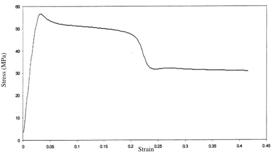
The typical mechanical response of a ductile semi-crystalline polymer to a tensile test is summarized in Figure 1.1-13. At low strains under εy, a nearly elastic deformation is

observed, where the strain ε is nearly proportional to the applied stress σ. This regime is characterized by an apparent slope E, which is generally taken as the Young’s modulus, neglecting the anelasticity. For higher levels of strain, the deformation becomes plastic and preferential orientation can be induced in the sample. The maximum of the stress strain curve is called the yield stress σy. When the plastically deformed and oriented part

(

)

γ

γ

2

T

T

T

l H

γ

=

−

∆

has extended to the whole sample being tested, a hardening can occur till the breakage of the material.

In semicrystalline polymers two cases should be considered in the stress-strain relationships. If the amorphous portion is rubbery, then the polymer will tend to have a low modulus, and the extension to break will be very large. If the amorphous portion is glassy, the polymer will behave much more like a brittle plastic. A schematic stress/strain curves are represented in Figure 1.1-14.

The cold drawing which appears after the yield point in Figure 1.1-14, comes from the rearrangement of the chains in a characteristic and complex manner, beginning with necking. A neck is a narrowing down of a portion of the stressed material to a smaller cross section. The necked region grows, at the expense of the material at either end, eventually consuming the entire specimen.

Figure 1.1-13 : schematic stress/strain curves for polymers. εy

stressσ

strainε σy

E

Figure 1.1-14 : schematic stress/strain curves for crystalline polymers stress

strain

Cold drawing

In the region of the neck, a very extensive reorganization of the polymer takes place. Spherulites are broken up, and the polymer becomes oriented in the direction of the stretch. The number of chain folds decreases, and the number of tie molecules between the new fibrils increases. The crystallization is usually enhanced by the chain alignment. At end of the reorganization, a much longer, thinner, and stronger fiber or film is formed.

The details of this plastic deformation behavior are always greatly dependent on the volume fraction of polymer which is crystallized (the degree of crystallinity), on the average size of the crystallites, and on the so-called tie molecules bridging the crystallites. In particular the yield stress of a semi-crystalline polymer is usually closely related to its degree of crystallinity, with highly crystalline polymers resembling stiff plastics and lightly crystalline polymers having a mechanical behavior resembling that of hard and dissipative elastomers. Therefore the degree of crystallization and hence the thermal treatment can dramatically influence the mechanical properties of a semi-crystalline polymer. This dependence of mechanical properties on the crystalline structure is however very specific of the polymer or copolymer and depends also on the processing conditions. We will discuss this aspect in much more detail for our specific polymer system in chapters 2 and 3.

1.2 Fracture behaviour of polymers

In this section, the fracture behaviour of polymers will be briefly summarized in order to build the theoretical background needed for the study of polymer adhesion. We first introduce some general theoretical concepts which will be useful to interpret the adhesion test we used in our study.

1.2.1 Introduction

The main emphasis of this section is upon the continuum approach where a polymer is considered as a continuum with particular physical properties but for which the molecular structure is mainly ignored.

The theoretical stress to cause cleavage fracture in a brittle solid is of the order of one-tenth of the Young’s modulus, E/10 (Kelly1). The modulus of a brittle polymer is typically 3 GPa, so the theoretical strength of such a material should be 300 MPa. Experimental results show that the measured fracture strengths of polymers vary between 10 and 100 MPa. This shortfall in strength was recognized many years ago by Griffith2 who showed that the relatively low strength of a brittle solid could be explained by the presence of flaws in the material, which act as stress concentrators.

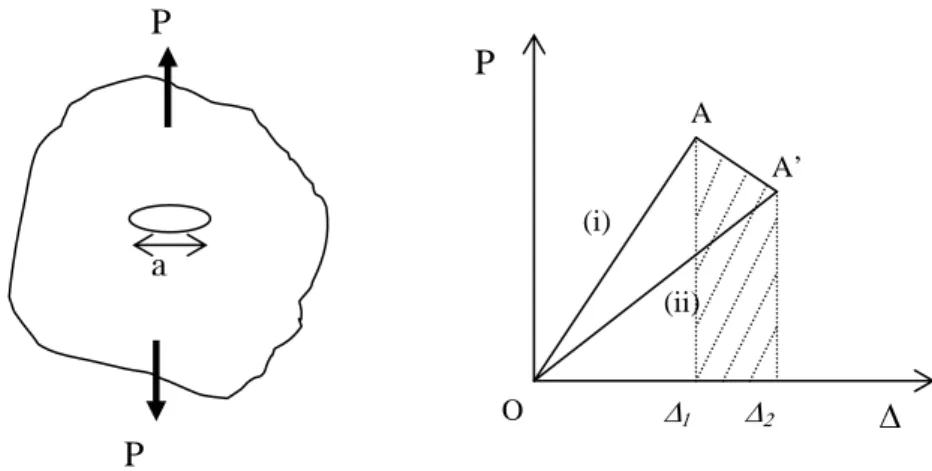
This situation can be easily described for materials which deform in a linear elastic manner. Figure 1.2-1 shows a simple case of an elliptic crack in a polymer sheet under a uniform applied stress σ0.

1_{Kelly, A. Stong solids. (Charendon Press, Oxford, 1966)}

The stress σt of the crack tip is after Williams 1 :

⎟⎟

⎠

⎞

⎜⎜

⎝

⎛

+

=

ρ

σ

σ

1

2

a

where ρ is the radius of curvature of the tip and 2a the major axis of the ellipse. A singularity appears clearly, when the hole becomes a crack, i.e. for ρÆ0 the stress goes to infinity. Modified approaches are needed such as the classical energy balance approach of Griffith or the stress intensity factor approach.

1.2.2 Energy balance approach

This approach is based on energy criterion and describes quasi-static crack propagation as the conversion of the work done W by an external force and the available elastic energy U stored in the bulk of the sample, into a surface free energy γ :

(

)

d W

U

dA

da

γ

da

−

≥

where dA is the increase in surface area associated with an increment of crack growth da. For a crack propagating in a thin sheet of thickness b, we obtain with dA = 2b.da :

1

Williams, J. G. Fracture Mechanics of Polymers. (Ellis Horwood Limited, New York, 1984)

(

)

1

2

d W

U

b

da

γ

−

≥

σ

However, for most polymers, the energy to propagate the crack is more than twice the value of the surface energy. This discrepancy comes from the fact that even in the most brittle polymer, a localised viscoelastic or plastic energy dissipation occurs, close to the crack tip, which is not taken into account in the value of 2γ .

The term 2γ may be replaced by the symbol Gc which will encompass all the energy

losses incurred around the crack tip. It is therefore the energy required to increase the crack by a unit length in a specimen of unit width. The fracture criterion then becomes :

Gc can be written as the sum of an intrinsic fracture energy G0 which is the energy

required solely for bond rupture and a term ψ, which corresponds to the energy dissipated in viscoelastic and plastic deformation at the crack tip. The value of ψ is usually the major contribution to the value of Gc.

We will now concentrate on materials which obey Hooke’s law, on which the concepts of linear elastic fracture mechanics (LEFM) can be applied.

Let us consider a crack of length a in the bulk loaded by a generalised force P (Figure 1.2-2).

The loading is represented by the linear load deflection curve (i), then, at point A, the crack grows so that the load and displacement changes (d∆ and dP), and finally the unloading would give curve (ii).

(

)

1

d W

U

G

G

b

da

−

=

≥

ψ

+

=

G

G

a

P

P

P

∆

Figure 1.2-2 : generalised loading of a cracked body which exhibits bulk linear elastic behavior.

The change in stored energy is the difference between the two integrated areas under the curves (i) and (ii) (the two triangles OA∆1 and OA’∆2) :

The external work, shown as the hatched area in Figure 1.2-2 is given by :

therefore

and by putting into equation 1.2-4 the crack propagation criterion becomes:

so by using the compliance C = ∆/P we get

with Pc as the load at the onset of crack propagation.

This equation is the foundation for many calculations of Gc, in particular in the case of the

double cantilever beam test, described in section 1.2.4.

1.2.3 The stress intensity factor approach

Before presenting the stress intensity factor approach, we should briefly recall the two limitary cases of stress and strain relevant to the fracture of material and the different modes of loading which will be encountered in the fracture of materials.

1.2.3.1

Plane strain, plane stress and different modes of fractures

There are two limitary cases of stress distribution particularly relevant to the fracture of materials. One is plane stress which is obtained in deformed thin sheets as shown in Figure 1.2-3. In a thin body, the stress through the thickness (σz) cannot vary appreciably

due to the thin section. Because there can be no stresses normal to a free surface, σz = 0

(

)

1

1

(

)

2

2

dU

=

U

−

U

=

P

+

dP

∆ + ∆ −

d

P

∆

1

2

dW

=

Pd

∆ +

dPd

∆

(

)

1

(

)

2

d W

−

U

=

Pd

∆ − ∆

dP

1

2

Pd

dP

G

b

da

da

∆ ∆

⎛

⎞

=

_⎜

−

_⎟

⎝

⎠

1

2

2

P dC

dC

G

b da

b C da

∆

=

=

throughout the section, a biaxial state of stress results. This is termed a plane stress condition.

Another important situation is the case where one of the three principal strains is equal to zero. This is often encountered in the constrained conditions around crack tips in relatively thick sheets. In a thick body, the material is constrained in the z direction due to the thickness of the cross section and εz = 0, resulting in a plane strain condition. Due to

Poisson’s effect, a stress, σz, is developed in the z direction.

A crack in a solid may be loaded in three different modes represented in Figure 1.2-4. The following discussion will then mainly be confined to a mode I loading, which is the situation encountered in our work.

Figure 1.2-3 : schematic representation of plane stress and plane strain.

mode I mode II mode III

1.2.3.2

Basic principles of the stress intensity factor approach

In the case of a sharp crack in a uniformly stressed infinite sheet shown in Figure 1.2-5 Westergaard1 has developed stress-function solutions which relate the local concentration of stresses at the crack tip to the applied far-field stress σ0.

For regions close to the crack tip the solution takes the form :

where σij are the components of the stress tensor at a point r, θ in polar coordinates.

Irwin2 has introduced the parameter K, which is the stress intensity factor. The solution then becomes :

From equation 1.2-12, it is obvious that for rÆ0 the stress goes to infinity, hence it is necessary to have a reasonable local fracture criterion. Irvin postulated that the following condition, KI>KIc, was a good failure criterion. This criterion has the advantage of being

independent of the detailed geometry of the sample far away from the crack tip. Any far-field loading situation would result in the same stress distribution but different intensities reflected by K.

Since the stresses at the crack tip are singular then clearly the yield criterion is exceeded in some zone near the crack tip region. However, if this zone is assumed to be small, the

1_{Westergaard, H. M. Journal of Applied Mechanics, A June: 46, (1939).} 2_{Irwin, G. R. Journal of Applied Mechanics, 29: 651-654, (1962).}

) ( 2 2 1 0

θ

σ

σ

( )

π

θ

σ

σ

elastic stress field will not be greatly disturbed. Dugdale1 assumed that yielding of the material at the crack tip makes the crack longer by the length of a plastic zone, R. The singularity at the crack tip is then cancelled out by a series of internal stresses of magnitude σp, usually taken to be the yield stress, σy, acting on the boundary of the

plastic zone as represented in Figure 1.2-6.

The length of the plastic zone is given by

and the thickness δ(r), of the plastic zone at any distance, r (θ=0°) is given by :

where

E* is the modulus which is equal to Young’s modulus, E, in plane stress and E/(1-ν2) in plane strain. The crack opening displacement, at the crack tip (r=0) is then given by

1.2.4 Relationship between G and K

In the case of LEFM a simple relationship exists between G and K, given in mode I by :

1

Dugdale, D. S. Journal of Mechanics and Physics of Solids, 8: 100, (1960).

2 8 I y K R

π

σ

( )

π

ξ

δ

σ

ξ

ξ

ξ

8

R

_K

E

E

σ

δ

π

σ

=

=

1.2.5 Experimental considerations

A basic aim of fracture mechanics is to provide a parameter, for characterizing crack growth, which is independent of test geometry. We will only present in this section the double cantilever beam geometry, which we used in this thesis. This test has been widely used to measure the fracture toughness at polymer interfaces since its reintroduction by Brown1 in the late 80’s.

In a standard cantilever beam test, a wedge of thickness ∆ produces a constant crack opening displacement as shown in Figure 1.2-7. When the crack is at equilibrium, the energy per unit area elastically stored in the deformed beam between the crack tip and the edge is equal to the fracture energy per unit area needed to propagate the crack.

The energy elastically stored in the bent part can be calculated from a classical calculation of the energy stored in a beam, bent by a point load P, which can be found in solid mechanics textbooks (Landau and Lifchitz2). We will only present the results of the calculation here.

1

Brown, H. R. Macromolecules, 22: 2859-2860, (1989).

2_{Landau, L. and Lifchitz, E. Théorie de l'élasticité. (Mir, Moscou, 1967)} 2 I I

K

G

E

=

for plane stress

(

)

1

K

G

E

ν

=

−

Figure 1.2-7 : the double cantilever beam geometry with a constant opening displacement.