HAL Id: hal-00876431
https://hal.archives-ouvertes.fr/hal-00876431
Submitted on 24 Oct 2013
HAL is a multi-disciplinary open access
archive for the deposit and dissemination of sci-entific research documents, whether they are pub-lished or not. The documents may come from teaching and research institutions in France or abroad, or from public or private research centers.
L’archive ouverte pluridisciplinaire HAL, est destinée au dépôt et à la diffusion de documents scientifiques de niveau recherche, publiés ou non, émanant des établissements d’enseignement et de recherche français ou étrangers, des laboratoires publics ou privés.
Improvement of RCS estimation of large targets by
using near-field approach
Erwan Gillion, Erwan Rochefort, Jacques Claverie, Christian Brousseau
To cite this version:
Erwan Gillion, Erwan Rochefort, Jacques Claverie, Christian Brousseau. Improvement of RCS esti-mation of large targets by using near-field approach. IEEE Radar Conference, Apr 2013, Ottawa, Canada. pp.1. �hal-00876431�
Improvement of RCS estimation of large targets by
using near-field approach
E. Gillion1,2, E. Rochefort2, J. Claverie1,3, C. Brousseau1
1
IETR – Institut d’Electronique et de Télécommunications de Rennes, UMR CNRS 6164, Université de Rennes 1, Rennes, France
2
CMN – Constructions Mécaniques de Normandie, Cherbourg, France
3
CREC St-Cyr, LESTP, Guer, France
Abstract—This paper presents a new method in order to
estimate the Radar Cross Section (RCS) of large objects in their environments. Object is defined as a volumetric surface and will be considered as a metallic target at a finite distance. This estimation is based on the use of dyadic Green’s function method which includes near-field issues. Simulations have been made in a frequency band between 1 to 20 GHz. Some simulated results of RCS estimation of a large metallic target taking into account the sea effect, are presented.
Index Terms—Radar Cross Section, Green’s function, near field
I. INTRODUCTION
In the remote sensing domain, one common application in naval electronic warfare is the radar detection of ships. This detection is based on the RCS (Radar Cross Section) measurement of the ship, which corresponds to its identity card. In the past, ship manufacturer measured the RCS after the ship was built. However, this method was too expensive and not efficient for ship manufacturers. Nowadays, it is more common to predict the RCS before building in order to comply with the specifications, and possibly, to modify the design to increase the stealthy behavior of the ship.
Over the past decades, numerous works have been done in order to estimate the RCS of objects [1]. This estimation is done by using electromagnetic (EM) methods like physical optic or physical theory of diffraction. Also, estimation is done considering the free space approximation. However, in the case of atmospheric phenomena and for large objects, usual methods do not reflect the reality [2]. In order to improve the RCS estimation, we propose to develop a method using a volumetric representation of the target, and taking into account its environment. Such representation introduces a near-field consideration in the scattered field.
This paper is organized as follows. In Section II, the classical RCS estimation is presented for a simple scatterer over the sea and taking into account the evaporation duct effect. Section III presents the limitation of the classical method applied to a large target and a solution to this problem is proposed. Finally, a validation of the proposed method is
realized in Section IV, showing the importance of the near-field consideration in the RCS estimation.
II. RCSOFASIMPLESCATTEREROVERTHESEA
A. RCS definition
The common formula to determine the RCS of a target is given by [1]: 2 2 2 0 lim 4 i s R R E E
where Ei and Es are respectively the incident and the scattered
fields, and R, the distance between the radar and the target. This expression is only true in free space and at infinite distance, but unsuitable in a real case. To match with a real case, apparent RCS app must be introduced [2]. That consists
of multiplying free space RCS, called 0, with the two-way
propagation factor which describes the influence of the environment:
4
0
.F
app
where the one-way propagation factor F is given by:
F
2
E
tot 2E
i 2 where Etot is the total field at the target location.
For a simple scatterer over a surface, this implies that the RCS variation is directly proportional to the two-way propagation factor’s variation.
B. Medium influence
In radar detection, especially over the sea surface, medium parameters have a strong impact on the apparent RCS value.
Figure 1. Impact of the sea roughness on the one-way propagation factor as a function of range, at a frequency of 5 GHz, and for different Douglas sea states. Radar and scatterer are located at a same heigth (10 m). Results are
compared to the standard case (flat sea and no duct).
The most significant effects are the sea roughness and the evaporation duct. Sea roughness describes the influence of sea waves on the diffusion of the EM waves, and evaporation duct traps the EM field within a surface-based waveguide.
Sea roughness effect modifies propagation factor and RCS proportionally to the sea state, as shown in Fig. 1. For a sea state lower than 3 (Douglas sea scale), results are similar to the flat sea case (Standard case). A decrease is observed for a sea state upper to 3.
Furthermore, evaporation duct effect increases or decreases propagation factor and RCS value, depending on radar range and target location. One example is presented at Fig. 2.We can see the duct effect on the propagation factor compared to the standard case (no duct).
Consequently, evaporation duct and rough sea must be considered together in RCS calculation. These two effects can work in the same way (decrease RCS) or in the opposite ways. Table 1 roughly summarizes interaction between sea roughness and evaporation duct for different Douglas sea scale.
TABLE I. DESCRIPTION OF THE IMPACT OF THE SEA ROUGHNESS AND THE EVAPORATION DUCT ON THE PROPAGATION FACTOR. Sea states Description Sea roughness Evaporation duct 0 Flat sea ø ++
1 – 2 Small sea waves – ++
3 – 4 Moderate sea waves + +
5 – 6 High sea waves ++ –
> 6 Very high sea waves ++ –
++. Very strong impact, +. Strong impact, –. Low impact, Ø. Inexistent
Figure 2. Impact of the evaporation duct on the one-way propagation factor as a function of range, at a frequency of 5 GHz, and for different height of the evaporation duct. Radar and scatterer are located at a same heigth (10 m).
Results are compared to the standard case (flat sea and no duct).
III. RCSOFALARGETARGET
A. Impact of altitude on RCS estimation
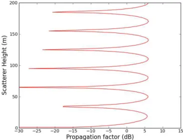
In this section, a large target is considered. In this case, the target is described by a set of scatterers or by meshed surfaces. For a standard case (no duct, flat sea), Fig. 3 shows that the height of the scatterer has an impact on its RCS. Indeed, according to (2), apparent RCS app of a multiple scatterers
located at different heights can vary from +12 dB to less than -30 dB.
Figure 3. One-way propagation factor as a function of scatterer height, at a distance of 10 km, for a propagation over the sea and at a frequency of 15 GHz, in a standard case (no duct, no roughness). Radar height is equal to
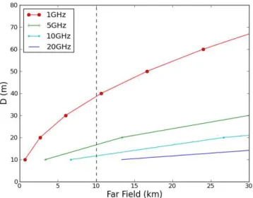
Figure 4. Minimum far-field range as a funtion of target dimensions D, for different frequencies.
However, most of naval targets are too large to assume that the scattered field is propagated in far-field conditions for the common range analysis, around 10 km. the usual Fraunhofer far-field criterion is given by:
d2 D. 2
where d, D and are respectively the minimum far-field distance, the largest dimension of the target and the wavelength. Thus, for large targets (more than 10 m), we observe an important increase of the far-field distance as the function of the frequency (Fig. 4). For example, for a target size of 40 m at the frequency of 1 GHz, a distance upper than 10 km is necessary to reach the far-field zone. Thus, in the case of large targets over the sea, like military vessels, the scattered field must be computed using near-field techniques depending on the range analysis.
Furthermore, usual way to consider RCS estimation is to use the reciprocity theorem [3]. However, as explained previously and depending on the range analysis, in some cases, the target size implies near-field assumption for the propagation from target to radar. Thus, the two-way propagation factor F4 must be divided into two one-way propagation factors (forward and backward), as shown in Fig. 5.
Moreover, in the case of near-field assumption in the scattered field, (1) cannot be used to estimate RCS of large target due to the non-respect of the far-field condition. Thus, to evaluate the RCS in this case, a more adapted expression, derived from the exact formula in near-field, must be used [4]:
2 * 4. . . 4 i S S app V H E Z R
Figure 5. Illustration of the forward and backward propagation.
where Vi is the magnitude of the transmitted field, Z, the
medium impedance and Hs*, the conjugate of the scattered
magnetic field.
In order to determine the apparent RCS app, a new
technique, taking into account the near-field formulation, is needed to compute Es.
B. Near-field method chosen : Dyadic Green function
The choice of the Dyadic Green function was performed by the following criteria:
This is an exact method, i.e. it includes near-field and far-field propagations. Propagation medium can also be taken into account.
This function is applicable in the 2D and 3D configurations.
The dyadic Green’s function for complex medium was developed from scalar Green’s function [5]. The scattered field computed by this method can be formulated as follows [6]:
V S S P j M P J M dV M E ( ) 0 ( , ) ( ) ( ) where = 2f is the pulsation of the EM field, 0, the
permeability of vacuum, Js, the surface current density on the
target surface, , the dyadic Green’s function, M, a point located on the source, and P, the location of the receiver.
By using (6) in (5), it is possible to obtain the RCS of a large target. However, before using such a method in real cases, canonical cases must be used to validate the method, assuming free space propagation condition.
IV. SIMULATIONRESULTS
To validate this method, simulation conditions are chosen in order to compare computed RCS with existing results [4] at the frequency of 15 GHz. A 1×1m perfectly conducting plate is simulated in order to measure the monostatic RCS at the normal incidence. Propagation of the EM field is done assuming the free space hypothesis.
An example of simulated results is shown in Fig. 6 and some interesting effects can be noticed. The most important effect is the presence of fluctuations located in the Rayleigh region. Theses RCS fluctuations imply the far-field approximation cannot be considered in this case. Moreover, for large targets, the measured RCS is mostly either in the Rayleigh region or the Fresnel region where the value of the RCS is not constant.
Figure 6. Free space monostatic RCS as a function of radar range for a 1×1m square plate , at normal incidence and at a frequency of 15 GHz.
Figure 7. Free space monostatic RCS as a function of radar range for a 10×10m square plate, at normal incidence and at a frequency of 1 GHz.
This result is in opposition with the far-field approximation usually used in the RCS calculation given in (2). Thus, this opposition confirms that the use of near-field method to calculate RCS of large target is necessary. To illustrate this phenomenon, simulated results with the free space dyadic Green’s function method, for a flat plate of 10×10 m dimensions at the frequencies of 1 and 10 GHz are presented on Fig. 7 and Fig. 8 respectively. According to previous observations, we observe that the more the frequency increases, the more the near-field frontier increases also. In this case, the near-field frontier is located around 180 m at 1 GHz, and moves to 1800 m at 10 GHz.
Furthermore, in Fig. 8, a comparison has been made between simulated results obtained from two metallic flat plates of 10×10 m and 30×30 m dimensions and for the same frequency of 10 GHz. We can see that the near-field region is extended to more than 10 km, corresponding to the usual range used for coastal radar. These observations show the importance of near-field computation in the RCS estimation of large target.
Figure 8. Free space monostatic RCS as a function of radar range for 10×10m and 30×30m square plates, at normal incidence and at a frequency
of 10 GHz.
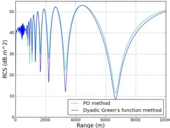
To have a more realistic approach, it’s then necessary to integrate the sea effect in the EM simulations. In order to validate our method in the presence of sea, a 1×1 m perfectly conducting flat plate is placed at 10 m above a flat sea. Then, the RCS is computed at the frequency of 10 GHz and compared to the results obtained from the physical optic (PO) method. Simulated results are presented in Fig. 9. The proposed dyadic Green’s function method shows a good agreement with the PO method. Moreover, this result shows an additional effect on RCS amplitude due to the target size.
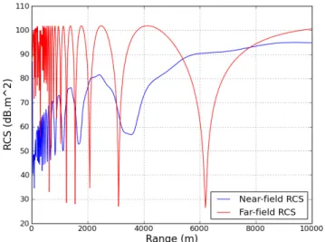
To illustrate these observations, a 10×10 m and 20×20 m flat plates are centered at 10 m above the sea level. Fig. 10 and Fig. 11 present the RCS of these plates compared to the theoretical far-field results obtained from (1) and (2) at the frequency of 10 GHz. Huge differences are observed between the far-field approach and the near-field approach (dyadic Green’s function method) in RCS results, especially for the lowest distances. These differences are due to the non-uniform illumination of the plate by the propagation factor (Fig.3).
Figure 9. Monostatic RCS as a function of radar range for a 10×10m square plate at normal incidence centered at 10 m above a flat sea, for a frequency
Figure 10. Monostatic RCS as a function of radar range for a 10×10m square plate at normal incidence centered at 10 m above a flat sea, for a frequency
of 10 GHz.
Figure 11. Monostatic RCS as a function of radar range for a 20×20m square plate at normal incidence centered at 10 m above a flat sea, for a frequency
of 10 GHz.
Thus, these presented results confirm that for the most usual naval applications, RCS calculation must take into account near-field propagation for the backscattered field.
Finally, Fig. 12 shows the impact of sea roughness on the RCS of a 20×20 m flat plate at 10GHz. We can see that the sea roughness implementation agrees with the previous discussion about its impact.
Figure 12. Monostatics RCS as e function of radar range for different Douglas sea state, for a 20×20m square plate, at normal incidence and for a
frequency of 10 GHz.
V. CONCLUSION
In this paper, a method for RCS estimation of large targets is presented and validated for canonical cases. Thus, RCS of a large object, like a ship, must be estimated taking into account the near-field approach for the backscattered field propagation. However, despite the improvement of RCS prediction for large targets, atmospheric effects have not been integrated in the dyadic Green’s function method and it was shown in this paper that the evaporation duct effect have an important impact on propagation factor and consequently on the RCS.
Then, our future work on dyadic Green’s function method in RCS prediction will include atmospheric parameters to improve accuracy of this model, and all results will be validated on real targets and by experimental data.
REFERENCES
[1] E. F. Knott, J. F. Shaffer and M. T. Tuley, “Radar Cross Section”, 1st ed., Artech House, New York, USA, 1985.
[2] J. Claverie and Y. Hurtaud, “Variation of the apparent RCS of maritime targets due to ducting effects”, AP2000 – Millenium Conference on Antennas and propagation, Davos, Switzerland, 9-14 April 200. [3] G. T. Ruck, D. E. Barrick, W. D. Stuart and C. K. Krichbaum, “Radar
Cross Section Handbook”, Plenum Press New York, 1970.
[4] P. Pouliguen, R. Hermon, C. Bourlier, J. F. Damiens, and J. Saillard, “Analytical formulae for Radar Cross Section of flat plates in near field and normal incidence,” Progress In Electromagnetics Research B, vol. 9, pp. 263–279, 2008.
[5] D.G. Duffy, “Green's functions with applications”, Chapman&Hall, CRC, 2001.
[6] C.T. Tai, “Dyadic Green’s function in Electromagnetic Theory”, 2nd ed., IEEE Press, 1993.