Multi Lyapunov Function Theorem Applied to a Mobile Robot Tracking a Trajectory in Presence of Obstacles

HAL Id: hal-01714868

https://hal.archives-ouvertes.fr/hal-01714868

Submitted on 23 Feb 2018

HAL is a multi-disciplinary open access

archive for the deposit and dissemination of

sci-entific research documents, whether they are

pub-lished or not. The documents may come from

teaching and research institutions in France or

abroad, or from public or private research centers.

L’archive ouverte pluridisciplinaire HAL, est

destinée au dépôt et à la diffusion de documents

scientifiques de niveau recherche, publiés ou non,

émanant des établissements d’enseignement et de

recherche français ou étrangers, des laboratoires

publics ou privés.

Multi Lyapunov Function Theorem Applied to a Mobile

Robot Tracking a Trajectory in Presence of Obstacles

Ahmed Benzerrouk, Lounis Adouane, Martinet Philippe, Nicolas Andreff

To cite this version:

Ahmed Benzerrouk, Lounis Adouane, Martinet Philippe, Nicolas Andreff. Multi Lyapunov Function

Theorem Applied to a Mobile Robot Tracking a Trajectory in Presence of Obstacles. European

Conference on Mobile Robots (ECMR 2009), Sep 2009, Dubrovnik, Croatia. �hal-01714868�

Multi Lyapunov Function Theorem Applied to a Mobile Robot

Tracking a Trajectory in Presence of Obstacles

Ahmed Benzerrouk, Lounis Adouane, Philippe Martinet and Nicolas Andreff

Abstract— In this paper, a reactive control architecture based on hybrid systems (continuous/discrete) is used to control a unicycle mobile robot tracking a given trajectory while avoiding obstacles. The main motivation of using hybrid systems is the possibility to define the overall control scheme as a combination of several elementary controllers (trajectory tracking, obstacle avoidance) that stability can be easily proved. However, there is a serious risk of oscillatory switching or even instability caused by random switch between these two elementary controllers. The contribution of this paper is to use the multiple Lyapunov functions (MLF) theorem to prove the global stability of a trajectory tracking task in presence of obstacles. To satisfy the MLF conditions, we propose to introduce a third controller in the architecture of control: the go-to-goal controller. Its role is to satisfy the second and the most difficult condition of MLF in a finite time. The approach is validated by numerical simulation.

I. INTRODUCTION

Controlling a nonholonomic mobile robot to follow a desired trajectory is a large topic of research investigated since a long time (see [10], [5], for instance). However, when controllers are developed for this specific task, it is important to take into account the environment variations. Indeed, it’s obvious that these controllers become easily useless and lead to collision when an obstacle appears on the robot’s way since they were only designed to track trajectory. However, the obstacle avoidance is not a problem anymore since it is widely investigated in the literature. Khatib [8] assumes that the robot moves in a potential field considering the objective to reach as an attractive point whereas the obstacle surfaces are repulsive fields.To minimize its local minima problems, circular potential fields were used [11]. Zapata and al [13] use a deformable virtual zone (DVZ) surrounding the robot thanks to proximity sensors: if an obstacle is detected, it will deform the DVZ and the approach is to minimize this deformation by modifying the control vector. These methods improve obstacle avoidance task but local minima problems were not completely solved. To perform the obstacle avoid-ance behavior, limit-cycle navigation proposed by Kim and Kim [9] can be used.

The unknown nature of the robot’s environment leads up to develop control architectures which guarantee a desired and a safe navigation in presence of obstacles. In fact, the intuitive idea to make a mobile robot able to avoid obstacles while tracking the desired trajectory is to have two simple controllers and to switch from one to another according to the robot’s relative position to the obstacle. Brooks [3] proposes a behavior based architecture where each layer accomplishes an elementary task. Therefore, it

becomes possible and important to study each controller and examine it independently from the whole control system. Theorems for hybrid systems seem consequently the most suitable to combine elementary controllers without loosing the global stability. Branicky in [2], shows that random switches between any stable systems do not guarantee the stability of the overall control. He consequently imposes restrictions on switching via multiple Lyapunov function. Moreover, with automata approach where each node gives the control law applied to the robot, hard switch may lead to the Zeno phenomenon [7] that exhibits an infinite number of discrete transitions between controllers in finite time. It potentially appears when the robot is on the boundary where the discrete event actuating switch becomes true. Effects caused by this phenomenon were shown by Egerstedt [6]. The latter regularizes its automaton by adding a node to overcome these undesirable effects: this node contains the sliding dynamics that is defined on the boundary between the two controllers. It comes to use more than one controller to control simultaneously the robot. The advantage of having each controller in a distinct node is then lost. Therefore, sliding dynamics seem not to be the optimal solution for robotics application. In this paper, it is proposed to apply theoretic study of multiple Lyapunov function to guarantee restrictions on switching. Adouane in [1], proposes to avoid this oscillatory switching between controllers commands while introducing a specific adaptation of each controller law. Here, our idea is to introduce a third controller (go-to-goal) which leads the robot on its trajectory after the obsta-cle avoidance step. This one allows to verify the multiple Lyapunov function theorem. Moreover, the used automaton is regularized by adding a third node corresponding to this controller: the go-to-goal node. Thus, undesirable effects are avoided without using sliding mode. The proposed automa-ton has then only one controller in each node. It will be proved that this controller achieves the desired task in a finite time.

The rest of this paper is organized as follows. In section II, we give the used mobile robot model and Individual con-trollers. Details on the multiple Lyapunov function theorem with its application in the proposed control architecture is given in section III. Convergence of the proposed architecture is proved in section IV. Simulation results, are given in section V. We conclude and give some prospects in section VI.

II. ROBOT MODEL AND ELEMENTARY CONTROLLERS

A. Robot model

Considering the unicycle mobile robot (cf. Figure 1), let

s,e and ˜θ be the state variables where s ∈ R and e ∈ R

are the Frenet frame coordinates (curvilinear and lateral coordinates respectively) of the center of the wheels axle, ˜

θ∈] − π, π] is the robot orientation with respect to the Xr

axis of the Frenet frame. Linear and angular velocities of the robot are respectively noted v and ω. The kinematic model of the unicycle can be described by the well-known equations (cf. Equation 1).

˙s =v.cos(˜_1−ec(s)θ)

˙e = v.sin(˜θ)

˙˜θ = ω − ˙sc(s)

(1)

where _c(s)1 is the curvature radius in the point

of coordinate s.

To accomplish a trajectory tracking task in presence of obstacles, a classical architecture of control has to contain a controller responsible of obstacle avoidance. Two main controllers are then requested.

B. Trajectory tracking controller

Consider the lateral and the angular errors of the robot

noted e and ˜θ respectively (cf. Figure 1). Tracking a reference

trajectory with a stable law means that e and ˜θ decrease

always to0. The following controller based on the Lyapunov

stability allows that. It is developed in [4] and is expressed as follows:

v= K

ω= −k1.v.e.sin ˜_θ˜θ− k2.|v| .˜θ+c(s)vcos˜_1−ec(s)θ

(2)

where K, k1 and k2 are positive constants. Its

candi-date Lyapunov function VT T = k1.e

2 2 +

˜ θ2

2 has a

decreas-ing time derivative. This controller asymptotically stabilizes

(e = 0, ˜θ= 0) provided that the robot is not on the singular

point e= _c(s)1 . Full demonstration is available in [4].

r

Y

X

s

O

θ

e

X

Y

O

Fig. 1. The mobile robot on the Frenet frame.

C. Obstacle avoidance controller

Limit cycle navigation method allows deciding in which direction and how far the robot avoids the obstacle. The limit

cycle is considered to be the circle characterized by Riradius

which is the radius of the hindering obstacle plus a safe margin. In order to focus the attention only on the proposed architecture of control, accurate details about this method are available in [9].

III. THE PROPOSED CONTROL ARCHITECTURE The proposed hybrid architecture is applied to a mobile robot which uses basic perceptual and decisional capabilities. Therefore, according to the robot’s sensors information, deci-sion to apply the convenient controller is made. The robot has to track trajectory while avoiding obstacles. Consequently, the architecture contains at least two controllers: trajectory tracking and obstacle avoidance. However, hard switches between these one may lead to instability even if each controller is individually stable. Therefore, more restrictions are needed to control these switches. Multiple Lyapunov function theorem [2] gives sufficient theoretic conditions to guarantee stability of an overall hybrid system. The proposed control architecture is based on it.

A. Multiple Lyapunov function theorem

Multiple Lyapunov function theorem (MLF)

Given N dynamical subsystems σ1, σ2,...,σN, each with

an equilibrium point at the origin, and N candidate

Lyapunov functions, V1, V2,...,VN. For each subsystem σi,

let t1, t2, ..., tm, ..., tk be the switching moments in this

subsystem (only one subsystem is active at a time).

If Vi decreases when σi is active and

Vi(tm) ≤ Vi(tm−1)

Then the hybrid system is Lyapunov stable.

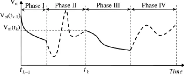
The theorem is illustrated (cf. Figure 2) for a simple

subsystem σi. Thus, when σi is active (phases I and III),

its Lyapunov function decreases. When the control switches

to another subsystem (phases II and IV), Vσi may increase.

However, to insure the global stability, this subsystem (and so as for all the other subsystems) must be reactivated only if its Lyapunov function takes a smaller value than the last time the system switches in.

Time

1 −

k

t

Phase I Phase II Phase III Phase IV

Vσi(tk-1)

k

t

Vσi

Vσi(tk)

Fig. 2. Variation of the Lyapunov function for the subsystem σi. Solid

In this paper, we prove that it is possible to use this theorem to guarantee stability of the robot control during all its navigation. Indeed, since the robot is controlled by a set of simple controllers whose stability is proved by the classical Lyapunov theorem, only the second condition of the above theorem needs to be satisfied.

If we assume that the mobile robot is able to reach its trajectory after achieving avoidance of each obstacle (which is not a heavy assumption since overlapped obstacles can be seen as one obstacle), the switching steps (Trajectory

tracking→ Obstacle avoidance →Trajectory tracking) form

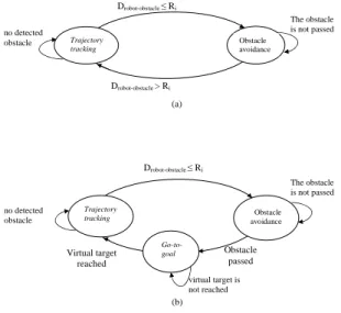
a new cycle for each obstacle. Then, we have to satisfy the second condition of MLF theorem for the trajectory tracking controller only since it is the only controller which appears two times in a cycle. Our idea is to use a specific "Go-to-goal" controller. This one is activated once the obstacle is avoided. Its role is to lead the robot on the reference trajectory until the MLF condition for the trajectory tracking becomes true. The proposed automaton is given (cf. Figure

3). Drobot−obstacle is the distance between the robot and

the obstacle, while Ri is defined in section (II-C). It is

obvious that undesirable effects due to fast switches between trajectory tracking and obstacle avoidance controller are removed. Indeed, when switching from obstacle avoidance in trajectory tracking, control has to go through go-to-goal. In practice, it is not possible to satisfy the MLF condition all the time. For example, when the robot is already on the

reference trajectory, VT T → 0. When it meets an obstacle,

VT T naturally increases since the robot leaves the reference

trajectory to avoid the obstacle. Go-to-goal can lead the robot on the reference trajectory again but its convergence is guaranteed only when time tends to infinity. In this paper, the go-to-goal controller designed by Toibero [12] is used. Here, we prove that this controller converges in a finite time, which is more interesting for practical application. Moreover, we will release the second constraint of MLF theorem in a

Drobot-obstacle > Ri Drobot-obstacle ≤ Ri Trajectory tracking Obstacle avoidance no detected obstacle (a) The obstacle is not passed Obstacle passed Virtual target reached Trajectory tracking Go-to-goal Obstacle avoidance Drobot-obstacle ≤ Ri The obstacle is not passed virtual target is not reached no detected obstacle (b)

Fig. 3. (a) Hard switches between controllers. (b)The proposed regularized automaton with go-to-goal controller.

suitable way such that we allow the control to switch in

trajectory tracking for the kthtime, when VT T(tk−1) ≈ 0.

B. Go to goal controller

The task to accomplish with this controller is to reach

a desired target. Here, (d, ˜θR) tend to (0,0), where d is

the robot-target distance and ˜θR is the robot orientation in

the relative robot frame (cf. Figure 4). control inputs are expressed as follows [12]

v= vmax

1+|d|dcos(˜θR)

ω= vmax

1+|d|cos(˜θR)sin(˜θR) + k2tanh(k3θ˜R)

(3) where v and ω are linear and angular velocities respectively.

Its time derivative ˙VGGis negative for all(d, ˜θR) 6= (0, 0).

This controller was shown globally asymptotically stable

using the Lyapunov function VGG=

˜ θ2R

2 + d2

2 [12]. Note that

it is possible to correct the final orientation of the robot when this one arrives to its goal simply by using the particular cas

of this control law with vmax = 0 (the robot corrects its

orientation without linear velocity) and the new control law becomes

v= 0, ω = k2tanh(k3θ˜R) (4)

C. Proof of convergence according to MLF theorem

Since it is assumed that after achieving each obstacle avoidance, the robot is able to reach its reference trajectory before eventually meeting an other obstacle, we have to prove that this task is achieved in a stable manner and in a finite time. It means that it is important to prove that switching from obstacle avoidance to trajectory tracking through go-to-goal controller arrives in a finite time. Trajectory tracking

controller is asymptotically stable. By noting xT T = (e, ˜θ)

(cf. Figure 1) andkxT Tk the Euclidian norm of xT T, and

by definition of asymptotic stability

∃δT T >0 : kxT T(0)k < δ1⇒ kxT T(t)k

t→∞

→ 0 If an obstacle is met, and once avoided, Go-to-goal

con-troller leads the robot to a point Pton the reference trajectory

Target

Robot

~

θ

O

d

(cf. Figure 5) until MLF condition is satisfied. Ptis defined

as the intersection of the trajectory with a virtual circle of

radius (Ri+ ǫ) where Ri is the circle of influence of the

obstacle. The latter is considered as avoided when the robot

is on the point Pe. Pe is the intersection of the influence

circle with its tangent going through Pt (chosen according

to the avoidance direction) (cf. Figure 5).

Go-to-goal is globally asymptotically stable (cf.

Subsec-tion III-B). By noting x2= (d, ˜θR) (cf. Figure 4), we have

∀δGG>0 : kxGG(0)k < δGG⇒ kxGG(t)k

t→∞

→ 0 Note that asymptotic stability cited above is insured when

t→ ∞. In practice, if the proposed architecture seems

allow-ing the robot to achieve obstacle avoidance and switchallow-ing in a stable manner, we have to prove that it is also done in a finite time. In general, switching in trajectory tracking controller

for the kth time tk occurs when VT T(tk) ≤ VT T(tk−1).

However, the worst case is when VT T(tk−1) is already

near to 0 (VT T(tk−1) → 0): How to decrease VT T again

to have VT T(tk) ≤ VT T(tk−1)? In this case, it comes

to lead up the robot until kxT Tk ≤ δT T. Hence, the

robot is in the convergence area of the trajectory tracking controller. Switching can then occur and stability is insured.

Moreover, note thatkxT T(tk)k ≤ VT T (for every k1≥ 1 (cf.

Subsection II-B), and the switch condition iskxT T(tk)k ≤ δ,

the constraint VT T(tk) ≤ VT T(tk−1) can then be released.

This case takes the maximum of convergence time since

kxT Tkhave to decrease until kxT Tk ≤ δT T whereas the

general case is kxT Tk ≤ VT T(tk) ≤ VT T(tk−1). We will

thus study this case proving that this time is still finite. We saw that trajectory tracking controller is asymptotically

stable provided that the lateral error satisfies e < _c(s)1 .

Since kxT Tk = (e, ˜θ), we can define the convergence area

of trajectory tracking controller as δT T = (eδ, ˜θδ) where

eδ = inf (_c(s)1 ), ˜θδ≈ 0. inf (_c(s)1 ) is the smallest curvature

radius of the reference trajectory. We have then to prove that Go-to-goal controller allows to arrive in this area in a finite time.

According to (cf. Figure 4) we get the simple equation of

Circle of influence yobst OA Ri+ε Ri XA xobst Pt Pe C Xr Yr _P’ t Reference trajectory YA Virtual target

Fig. 5. Virtual target to reach before reactivating trajectory tracking

controller.

the derivative ˙˜θR

˙˜θR= v

sin(˜θR)

d − ω (5)

Since the objective is to lead the robot to δ1, d ≈ 0 but

d6= 0. ˙˜θR is then defined.

By replacing v and ω from (3) in (5) we get:

˙˜θR= −k2tanh(k3θ˜R) (6)

It can be noticed from (6) that the variation of ˜θR is

independent from d. Thus, if time of convergence of the

Go-to-goal controller is noted Tf, its maximum is obtained if

first ˜θRdecreases , and only when ˜θRconverges, the distance

robot-target d starts decreasing. It can be concluded that

Tf ≤ (∆t1+ ∆t2)

where ∆t1 is the convergence time of ˜θ to 0 (it is the time

of convergence of ˜θRto 0 plus the time of convergence of ˜θ

to 0 knowing ˜θR= 0) and ∆t2is the convergence time of d

(it will be shown later that it means decreasing of e to eδ).

Hence, if∆t1 and∆t2 are finite, Tf is finite, too.

1) ∆t1is finite: The angle ˜θR is such that ˜θR∈] − π, π].

We decompose the interval into two parts: ˜θR≥ 0 and ˜θR≤

0. Let us study the case ˜θR≥ 0 :

from (6) we get: ˙˜θR≤ 0. It means that ˜θR is decreasing.

It can be noticed that max(∆t1) is when ˜θR→ π (since

max(˜θR) = π).

An important property of tanh(k ˜θR) is that

tanh(k ˜θR) → 1 for every angle ˜θR >> 0 and with a

well chosen k. Let us consider that ˜θR >>0 if ˜θR >10◦.

Thus, by replacing in (6) we get ˙˜θR ≈ −k2(1 − ǫ1) where

ǫ1<<1.

A simple integration gives

δt1=

˜

θR(t) − ˜θR(t0)

−k2(1 − ǫ1)

After a time δt1, ˜θRbecomes small, we can therefore make

the assumption

tanh(k3θ˜R) = k3θ˜R

thanks to a Taylor development of the function tanh of

order 1. when we replace in (6) we get: ˜

θR(t2) = ˜θR(t1)e−k2k3(t2−t1)

It means that ˜θR is exponentially decreasing. In addition,

˜

θR(t1) is already small. Consequently it rapidly decreases

and we can make the approximation that: ∆t1 = δt1+ δ

where δ is time of convergence of ˜θ to0 knowing ˜θR= 0 .

In other words, when the robot arrives to the virtual target,

it has to correct its final orientation to have ˜θ≤ ˜θδ. This is

accomplished thanks to the controller (cf. Equation 4) when

the linear velocity v= 0 as cited. Details will not be given

since it is done in the same way as for ˜θR. Demonstration

is also given only for one interval. For the second interval

2) ∆t2 is finite: The variation of d can be written ˙ d= −vcos(˜θR) = − vmax 1 + ddcos 2_(˜θ R) (7)

After ∆t1, θ˜R is sufficiently small to write

cos2_(˜θ R) = 1 − ǫ2 (ǫ2<<1). By replacing in (7), we get ˙ d= −vmax 1 + dd(1 − ǫ2) where ( ˙d= dd_dt)

The solution of this differential equation gives

∆t2=ln(d(t)) + d(t) − ln(d(t0)) − d(t0)

−vmax(1 − ǫ2)

(8) Note also that the relation between the lateral error e and the distance d can be easily deduced (cf. Figure 5). Indeed, when switching in trajectory tracking, lateral error according

to Pt (cf. Figure 5) is

e= dsin(φ)

where φ=PtPˆePt′, where P

′

t is the projection of Pt on

the Xr axis (of the Frenet frame).

The worst case to switch in trajectory tracking for the kth

time tk is when VT T(tk−1) ≈ 0 and the curvature radius in

Ptis inf(c(s)1 ). max(∆t2) can then be calculated as:

∆t2= ln(inf( 1 c(s)) sin(Φ) ) + inf( 1 c(s)) sin(Φ) − ln(d(∆t1)) − d(∆t1) −vmax(1 − ǫ2)

Note that c(s) 6= 0 (otherwise, the curvature radius

inf( 1

c(s)) = ∞ which means in practice that there is no

singularity, and switching in trajectory tracking can occur

everywhere). ∆t2 is then finite too. Since we saw above

that Tf, the whole time of convergence is Tf <∆t1+ ∆t2

Tf is then finite, too. In next section, numerical simulation

confirms the stability of the proposed control architecture. IV. SIMULATION RESULTS

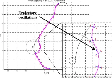
To estimate the relevance of the proposed hybrid archi-tecture, we compare it with results given by hard switches between the two controllers: trajectory tracking and obstacle avoidance. Results are shown in (Fig. 6). We can notice that when detecting the obstacle, the robot switches effec-tively in obstacle avoidance. However, when the obstacle is passed, the robot switches in trajectory tracking controller and oscillations are observed. Indeed, the robot (which is now controlled by trajectory tracking command) falls in the circle of influence again and tries to avoid it (switch in obsta-cle avoidance again). Variations of Lyapunov functions are illustrated in (Fig. 7) with switching control indicator. The latter indicates which controller is active (its values are 1 and 2 for trajectory tracking and obstacle avoidance respectively). We can notice that undesirable switches are occurring and MLF condition is not satisfied. Indeed, unless geometrical constraints (distance of the robot to the obstacle), there is no rules managing these switches. Moreover, the Lyapunov

-20 -15 -10 -5 0 5 10 15 20 0 5 10 15 20 25 30 35

Robot trajectory in the [O, X, Y] reference

X [m] Y [ m ] -7 -6 -5 -4 -3 -2 -1 10 11 12 13 14 15 16 17 Trajectory oscillations

Fig. 6. Real robot’s path controlled by hard switches. The surrounded area is enlarged on the right.

0 50 100 150 0 10 20 30 40 50

60 Lyapunov functions variation of the two controllers.

V 0 50 100 150 0 0.5 1 1.5 2

2.5 Switching control indicator.

1:trajectory tracking controller, 2:Obstacle avoidance controller (a) (b) t0 t1 V(t0) V(t1) V(t1)> V(t0)

Fig. 7. Lyapunov function variations of the two controllers.

function VT T is decreasing every time the controller is active,

however the second MLF condition is not satisfied.

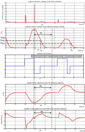
On the other side, our architecture of control (cf. Section III) allows avoiding these useless switches thanks to go-to-goal controller. The latter prevents hard switches from occur-ring before that the obstacle is passed. The real path followed by the robot is shown in (Fig. 8) where no oscillation is observed. The robot has to avoid two obstacles. According to their positions, It avoids the first counter clockwise while the second is avoided in a clockwise direction. Switch moments (cf. Figure 9) with Lyapunov functions progress of the active controller are given in (a). It can be noticed that the Lyapunov function of each controller is decreasing when this one is active (first condition of MLF). Lyapunov function of the trajectory tracking controller is given in (b). Switch moments are illustrated. It is noticed that switch occurs at the moments

t2 and t1 where VT T(t2) < VT T(t1) < VT T(t0= 0), which

is due to the second condition of MLF. Note that in (c), the value 0 of the switching control indicator refers to the added controller Go-to-goal. Finally, lateral and angular errors are

given in (d) and (e) respectively: It is shown that Tf <<

-20 -15 -10 -5 0 5 10 15 20 25 0 5 10 15 20 25 30 35

Robot trajectory in the [O, X, Y] reference

X [m] Y [ m ] -5 -4 -3 -2 -1 0 8 9 10 11 12 13 14 15 16 Non holonomic constraints Obstacles Trajectory to follow

Fig. 8. Real robot path when controlled with the proposed control

architecture. The surrounded area is enlarged on the right.

there was no need to maintain Go-to-goal controller until

e < eδ and ˜θ≈ 0.

V. CONCLUSIONS AND FUTURE WORKS We applied hybrid control architecture on a mobile robot to obtain a stable trajectory tracking while avoiding obsta-cles. Indeed, the robot is controlled by elementary contin-uous controllers according to the sub-tasks to accomplish (trajectory tracking, obstacle avoidance) and switching from a controller to an other is done referring to discrete events. We saw that hard switches are not efficient to insure global stability. Therefore, we propose to design a stable hybrid con-trol architecture. In addition to elementary stable concon-trollers for the two main sub-tasks, we introduce a third controller which overcomes different constraints (second condition of the multiple Lyapunov function theorem, singularities of trajectory tracking controller). Simulations show that our architecture prevents useless switches, guaranteeing thus a suitable navigation for the robot. Application to multi-robot systems navigating in formation will be done. The objective is to make each robot able to avoid an obstacle before regaining the formation.

REFERENCES

[1] L. Adouane. An adaptive multi-controller architecture for the navi-gation of mobile robot. In 10th IAS, Intelligent Autonomous Systems, pages 342–347, Baden-Baden, Germany, July 2008.

[2] M. S. Branicky. Stability of switched and hybrid systems. In 33rd

IEEE Conference on Decision Control, pages 3498–3503, 1993.

[3] R. A. Brooks. A robust layered control system for a mobile robot.

IEEE Journal of Robotics and Automation, 2:14–23, 1986.

[4] C. Canudas de Wit, B. Siciliano, and G. Bastin. Theory of Robot

Control. Springer Verlag Edition, 1996.

[5] B. D Andrea-Novel, G. Campion, and G. Bastin. Control of non-holonomic wheeled mobile robots by state feedback linearization.

International Journal of Robotics Research, 14(6):543559, 1995.

[6] M. Egerstedt, K. H. Johansson, J. Lygeros, and S. Sastry. Behavior based robotics using regularized hybrid automata. Computer Science

ISSN 0302-9743, 1790:103–116, 2000. 0 20 40 60 80 100 120 140 160 0 2 4 6 8 10 12 14 16

Lyapunov function variation of the trajectory tracking controller

Time (s) V 0 20 40 60 80 100 120 140 160 0 5 10 15 20

Switching control indicator

Time (s) 0:go to goal controller, 10:trajectory tracking controller, 20:Obstacle avoidance controller

(a) (b) 0 20 40 60 80 100 120 140 160 -4 -3 -2 -1 0 1 2 3 Time (s) e ( m )

variation of the Lateral error (e) to the reference trajectory

(d) 0 20 40 60 80 100 120 140 160 0 20 40 60 80 100 120 140

Lyapunov functions variation of the three controllers.

Time (s) V o f th e a c tiv e c o n tr o lle r (a) (b) (c) 0 20 40 60 80 100 120 140 160 -150 -100 -50 0 50 100

Variation of the angular error according to the reference trajectory

Time (s) T h e ta T ild e ( °) (e) ∆t1 ∆t2 Tf t1 t2 VT T V(t0) V(t1) V(t2) 0 20 40 60 80 100 120 140 160 -0.5 0 0.5 1 1.5 2 2.5

Switching control indicator.

0:go to goal controller, 1:trajectory tracking controller, 2:Obstacle avoidance controller

Fig. 9. Lyapunov variation functions of the proposed control architecture.

[7] K. H. Johansson, M. Egerstedt, J. Lygeros, and Sastry S. On the regularization of zeno hybrid automata. Systems & Control Letters, 38:141–150, 1999.

[8] O. Khatib. Real time obstacle avoidance for manipulators and mobile robots. International Journal of Robotics Research, 5:90–99, 1986. [9] D. Kim and J. Kim. A real-time limit-cycle navigation method for

fast mobile robots and its application to robot soccer. Robotics and

Autonomous Systems, 42:17–30, 2003.

[10] C. Samson. Control of chained systems application to path following and time-varying point-stabilization of mobile robots. IEEE

transac-tions on automatic control, 40(1):64–77, 1995.

[11] M.G. Slack. Navigation template: mediating qualitative guidance and quantitative control in mobile robots. IEEE Transactions on Systems,

Man and Cybernetics, 23(2):452466, 1993.

[12] J.M. Toibero, R. Carelli, and B. Kuchen. Switching control of mobile

robot for autonomous navigation in unkown environments. IEEE

International Conference on Robotics and Automation, pages 1974–

1979, 2007.

[13] R. Zapata and P. Lepinay. Reactive behaviors of fast mobile robots.