HAL Id: tel-00839910
https://tel.archives-ouvertes.fr/tel-00839910
Submitted on 1 Jul 2013HAL is a multi-disciplinary open access
archive for the deposit and dissemination of sci-entific research documents, whether they are pub-lished or not. The documents may come from teaching and research institutions in France or abroad, or from public or private research centers.
L’archive ouverte pluridisciplinaire HAL, est destinée au dépôt et à la diffusion de documents scientifiques de niveau recherche, publiés ou non, émanant des établissements d’enseignement et de recherche français ou étrangers, des laboratoires publics ou privés.
Formes curvilinéaires avancées pour la modélisation
centrée objet des écoulements souterrains par la
méthode des éléments analytiques
Philippe Le Grand
To cite this version:
Philippe Le Grand. Formes curvilinéaires avancées pour la modélisation centrée objet des écoulements souterrains par la méthode des éléments analytiques. Sciences de l’environnement. Ecole Nationale Supérieure des Mines de Saint-Etienne; Université Jean Monnet - Saint-Etienne, 2003. Français. �NNT : 2003EMSE0009�. �tel-00839910�
n
Ecçl.e . Nation.ale
-~,
.;..-Supeneure des Mmes
··-n
SAINT-ETIENNE
THE SE
présentée par
Philippe LE GRAND
pour obtenir le grade de
Docteur
de l'Ecole Nationale Supérieure des Mines de Saint-Etienne et de l'Université Jean Monnet
Spécialité Science de la terre et de l'environnement
Formes curvilinéaires avancées pour la modélisation centrée objet
des écoulements souterrains
par la méthode des éléments analytiques
Advanced curvilinear shapes for object centered modeling
of groundwater flow with the analytic element method
Soutenue le 4 Avril 2003 devant le jury composé de : Dr. R.J. Barnes Pr. M. Razack Pr. O.D.L. Strack Dr. M. Batton-Hubert Dr. D. Graillot Année 2003 président rapporteur rapporteur examinateur examinateur N° d'ordre: 3101D
~
Ec·ole
Nationale
-~'
l,_.Supérieure des Mmes
.--"1:1
SAINT-ETIENNE
THE SE
présentée par
Philippe LE GRAND
pour obtenir le grade de
Docteur
de l'Ecole Nationale Supérieure des Mines de Saint-Etienne et de l'Université Jean Monnet
Spécialité Science de la terre et de l'environnement
Formes curvilinéaires avancées pour la modélisation centrée objet
des écoulements souterrains
par la méthode des éléments analytiques
Advanced curvilinear shapes for object centered modeling
of groundwater flow with the analytic element method
Soutenue le 4 Avril 2003 devant le jury composé de : Dr. R.J. Barnes président
Pr. M. 'Razack rapporteur Pr. O.D.L. Strack rapporteur
1
Dr. M. Batton-Hubert examinateur Dr. D. Graillot examinateur
Année 2003 N° d'ordre: 3101D
ii
Acknowledgements
Espace
Fa
urie]The present work would not have been possible without the support and encouragement of many people, so many that they cannot all be included here. Those whom I omit know who they are, and the extent of my gratitude.
I wish to thank Professor Moumtaz Razack, from the Université de Poitiers, for kindly accepting the role of reviewer of this work.
Professor Otto Strack, from the University of Minnesota, must accept my most profound thanks, as a reviewer of this dissertation, and as the most constant source of support, encour-agements, comments and challenges throughout my post graduate studies. I am gratefully in his debt.
Dr. Randal Barnes, associate professorat the University of Minnesota, earned my gratitude in many ways. His direction while advising me on my Master's degree, his patience with a strong headed student, his challenging my ideas, and his comments on the work included here or elsewhere have all been crucial in teaching me to do research. For all that, for his hosting me as an exchange student and researcher, and for his acceptance to participate in the jury for this thesis, I am thankful.
Professor Philippe Davoine, now retired from the Ecole des Mines, introduced me to water issues in general, and groundwater by consequence, as well as the art of teaching, which he has mastered. His wit, his intelligence, and his witness to the quality that an individual can reach as a researcher have allled me clown the academie path. My sincere thanks accompany him.
Dr. David Steward, Kansas State University, deserves to have his work acknowledged here. Without his excellent counsel, his encouragements and other support, the present dissertation would not have come to an end on time.
My co-advisor, Dr. Mireille Batton-Hubert, researcher at SITE, has the capacity to push my refl.ections further, to force me to put my thoughts into words, and to make me explore areas of science from which I might have shyed away otherwise. How I wish I had recorded sorne of our discussions! I am grateful for her presence and support.
my advisor in this process, Dr. Didier Graillot, research director and head of the center SITE, deserves my deepest thanks. Besicles securing the financial means without which I could not have continued a life in research. His creativity, and his willingness to deal with the ad-ministrative complications of a student whose heart was overseas are all commendable; his open-mindedness, his experience and his capacity to perceive the larger picture were instru-mental Jn giving me the freedom, and the bounds, that I needed.
Remerciements
SCIDEAf
Espace
Fauriel:
m
Le présent travail n'aurait pas été possible sans le soutien et les encouragements d'un grand nombre de personnes, trop grand pour qu'ils soient tous inclus ici. Ceux que j'omets savent qui ils sont, et l'étendue de ma gratitude.
Je souhaite remercier le professeur Moumtaz Razack, de l'Université de Poitiers, pour avoir accepté le rôle de rapporteur sur mon travail.
Professeur Otto Strack, de l' University of Minnesota, doit accepter mes plus profonds remerciements, comme rapporteur sur ce mémoire, et comme la source la plus constante de soutien, d'encouragements, de commentaires et de mises à l'épreuve tout au long de mes études de troisième cycle. Avec gratitude, je lui suis redevable de beaucoup.
Dr. Randal Barnes, professeur associé à University of Minnesota, a gagné ma gratitude--de nombreuses façons. Son instruction alors qu'il me dirigeait durant mon Master of Science, sa patience avec un étudiant têtu, sa mise à l'épreuve de mes idées, ses commentaires, sur les travaux inclus ici ou ailleurs, ont tous été cruciaux pour m'apprendre à faire de la recherche. Pour tout cela, pour son accueil quand j'étais étudiant, puis chercheur, en échange, et pour son acceptation à prendre part au jury de cette thèse, je le remercie.
Professeur Philippe Davoine, aujourd'hui retraité de l' Ecole de Mines, m'a ouvert l'esprit aux problèmes de l'eau en général, et aux eaux souterraines par conséquent, ainsi qu'à l'art de l'enseignement, dont il était maître. Son esprit, son intelligence, et son témoignage de la qualité que peut atteindre un individu en tant que chercheur m'ont tous conduit vers une carrière académique. Mes sincères remerciements l'accompagnent.
Dr. David Steward, de Kansas State University, mérite de voir ses efforts reconnus ici. Sans son excellent conseil, ses encouragements et autres soutiens, le présent mémoire n'aurait jamais vu le jour.
Ma co-directrice, Dr. Mireille Batton-Hubert, maître de conférence à SITE a eu la capacité à pousser mes reflexions plus loin, a me forcer à exprimer mes pensées, et à me faire explorer des secteurs scientifiques que j'aurais autrement évités avec timidité. Comme je regrette de n'avoir pas enregistré certaines de nos conversations! Je suis reconnaissant de sa présence et de son soutien.
Mon directeur de thèse, Dr. Didier Graillot, directeur de recherche et directeur du centre SITE, mérite mes profond remerciements. En plus de la fourniture des moyens financiers sans lesquels je n'aurais pas pu poursuivre ma vie de chercheur, sa créativité et sa volonté de gérer les complications administratives liées à un étudiant dont le coeur était à l'étranger sont toutes louables. Son ouverture d'esprit, son expérience et sa capacité à percevoir la vue d'ensemble ont contribué à me donner la liberté, ainsi que les limites, qui m'étaient nécessaires.
iv
Summary
Using GIS for the design of groundwater models motivates the search for numerical methods that do not require the discretization of the flow domain: GIS are natively vectorized.
Numerical methods that relie on the discretization of the boundaries rather than the domain offer the advantage of retaining the native description of information in vector form as provided by the GIS, thus reducing the loss inherent to raterization and subsequent vectorization. The Analytic Element Method is especially promising. However, it lacks the capacity to handle a specifie type of object, NURBS curves.
The functions necessary to allow the inclusion of these curves in the AEM are derived, and examples are provided. Their versatility is presented, also showing that existing smooth curves can be represented as NURBS, thus allowing backward compatibility, should they be replaced. A method is offered to allow for faster model response when using these curvilinear elements, based on the Direct Boundary Integral Method. Standard line elements are also improved to allow greater precision and control in the speed-improving scheme.
Keywords: GIS, analytic elements, curvilinear elements, NURBS, Direct Boundary Integrais
Résumé
L'utilisation des SIG pour la conception de modèles d'écoulements souterrains motive la recherche de méthodes numériques qui ne requièrent pas la discrétisation du domaine de l'écoulement : les SIG sont par nature vectorisés.
Les méthodes numériques qui se fient à la discrétisation des frontières plutôt que du domaine offrent l'avantage de garder le description originale de l'information sous forme vecteur, telle que fournie par le SIG, réduisant ainsi les pertes inhérentes à la rastérisation et la vectorisation ultérieure. La méthode des éléments analytiques est particulièrement prometteuse. Cependant, il lui manque la capacité à gérer un type spécifique d'objets, les courbes NURBS.
Les fonctions nécessaires à l'inclusion de ces courbes dans le cadres de l' AEM sont dérivées, et des exemples sont fournis. Leur souplesse est présentée, et on montre que les formes courbes existantes dans l'AEM peuvent être représentées par des NURBS, permettant ainsi la compa-tibilité, si elles devaient être supplantées.
Une ,méthode est proposée pour améliorer le temps de réponse des modèles lorsque les éléments curvilinéaires sont utilisés, basée sur la méthode des intégrales frontières directes. Les éléments linéaires classiques sont également améliorés pour permettre meilleurs précision et contrôle dans la technique d'accélération.
Mots clef : SIG, éléments analytiques, éléments curvilinéaires, NURBS, Intégrales Frontières Directes
Contents
1 Introduction
1.1 On the approach
1.2 On notation and symbols . 1.3 On the use of English . . .
1 Introduction- version française
1.1 De l'approche . . . . 1.2 De la Notation et des symboles 1.3 De l'utilisation de l'Anglais . .
2 GIS and Modeling in hydrogeology
2.1 Tools of hydrogeological modeling . . . . 2.1.1 The three sides of modeling groundwater flow 2.1.2 GIS: Geographie Information Systems . . . ..
2.1.3 An Observation- Modeling: process centered activity 2.2 Object centered modeling
2.2.1 Concept . . . .
2.2.2 Advantages and drawbacks .
2.2.3 A method for object centered modeling of groundwater flow
3 The Analytic Element Method
3.1 Fundamental concepts of the AEM . . . . 3.1.1 Position of the AEM compared to other numerical techniques 3.1.2 Foundations of the method . . . . . .
v 1 2 3 3 5 6 7 8 9 11 11
14
14
15
15
16 17 21 23 23 26CONTENTS Vl
3.1.3
Basic elements33
3.2
Recent Advances...
41
3.2.1
Over-specification .41
3.2.2
Superblocks....
43
3.2.3
Curvilinear elements43
3.2.4
Not-So-Analytic Elements ?44
3.3
Examples of basic elements . . .46
4 Analytic elements along curved shapes 49
4.1
Curvilinear shapes in the Analytic Element Method51
4.1.1
Reason for existence51
4.1.2
The circular arc . .52
4.1.3
The hyperbolic arc53
4.1.4
Remarks . . .54
4.2
. B-Splines shaped boundaries .55
4.2.1
An introduction to B-Splines .55
4.2.2
Relating NURBS curves to Rational Bézier curves59
4.2.3
Existing curvilinear shapes as Bézier curves61
4.3
Complex Potential of Spline-shaped elements .63
4.3.1
The line-dipole. . .
64
4.3.2
Cauchy Singular Integral over Rational Bézier curves66
4.3.3
Computing the discharge function .68
4.4
Evaluation issues..
68
4.4.1
Special points69
4.4.2
Roots of polynomials72
4.5
Solving a boundary value problem along a spline .73
·1
4.5.1
Representativeness of the Dirichlet problem74
4.5.2
Setting up the resolution matrix .74
4.5.3
On Jump-specified elements78
CONTENTS
5 Computational efficiency of curvilinear elements
5.1 Polygonal Far-Fields . . . . 5.1.1 Direct boundary integral over a polygon 5.1.2 Polygon refinement
5.1.3 Examples . . .
5.2 Line Elements of very large degree. 5.2.1 Double-Root line-elements .
5.2.2 Improving High Degree Line Element
6 Conclusion 6.1 Summary 6.2 Extensions . 6.2.1 6.2.2 6.2.3
Relating model Inputs to Outputs .
Interface elements for the combination of resolution methods Beyond hydrogeology . . . .
6 Conclusion - version française
6.1 Bilan . . . . 6.2 Extensions .
6.2.1 Lier entrées et sorties de modèles 6.2.2 Eléments interface
pour l'association de méthodes de résolution 6.2.3 Au delà de l'hydrogéologie . . . . vii 83 85 85 87 88 95 95
104
109109
110
110
110
110
113113
114
114
114
115
List of Figures
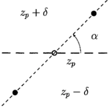
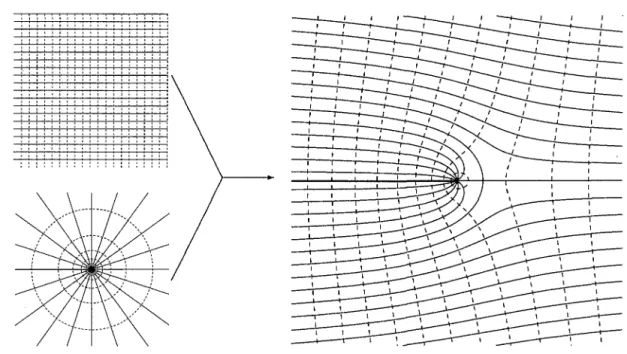
3.1 Setup for derivation of a line dipole . . . 37 3.2 A wellin uniform flow, produced by superposition of solutions 3.30 and 3.28 38
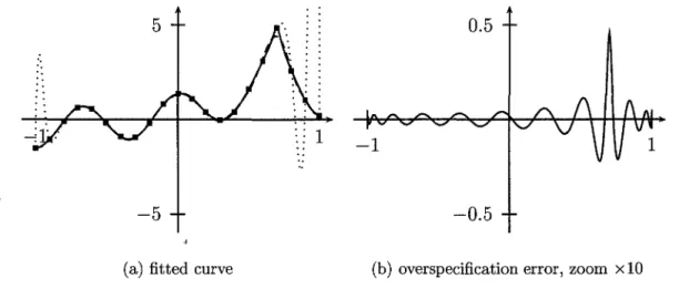
3.3 Collocation vs. Over-specification 41
(a) fitted curve . . . 41
(b) overspecification error, zoom x10 41
3.4 Isolated constant strength line-sink . 4 7
3.5 Impermeable barrier in uniform flow 47
3.6 Zone of low permeability . . 48
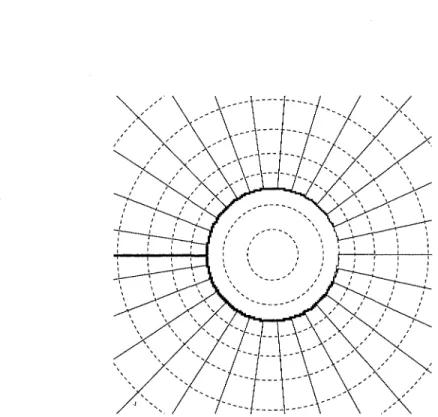
3. 7 Circular area of infiltration . 48
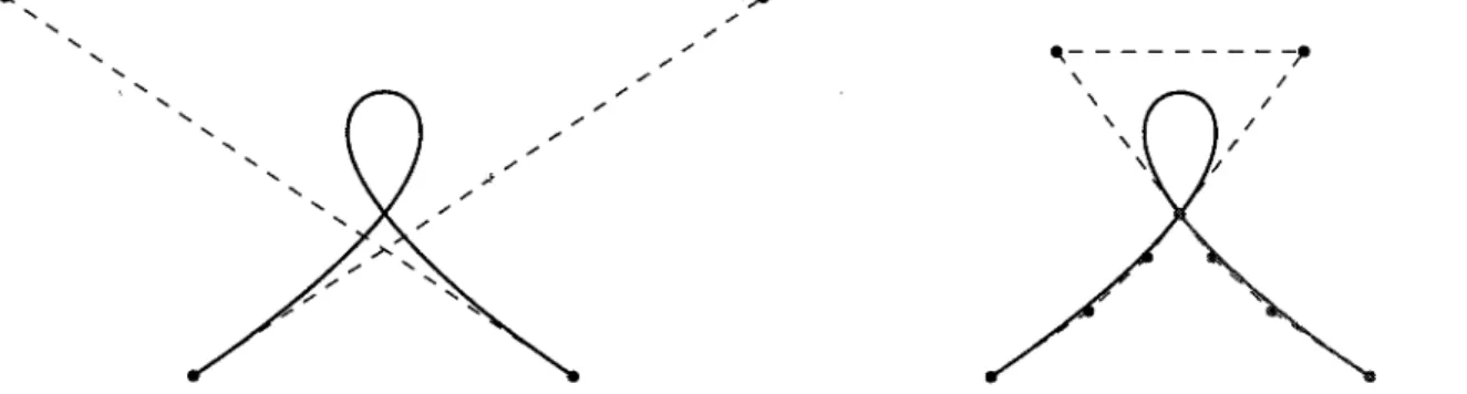
4.1 Looping spline . . . .
4.2 Line-sink and possible locations of the branch cuts . 4.3 Impermeable curvilinear barrier
4.4
(a) general view . (b) zoom on tip .
( c) zoom on well location Lakes in uniform flow . , (a)
(b)
general view . . .
zoom on western tip of northern lake 1 ( c) zoom on narrow section between the lakes
5.1 Hull and polygon associated with a general NURBS curve
(a) general convex hull . . . .
lX 58 75 80 80 80 80 81 81 81 81
89
89
LIST OF FIGURES
(b) hull refined by subdivision 5.2 Rational Bézier Curve hulls .. 5.3 Tip vertex displacement method .
5.4 Moving polygon vertices away from the curve (a) regular points .
(b) inflexion points 5.5 General flow field ..
5.6 Flow field with the curvilinear barrier .
5.7 Logarithm of absolute error for a refined polygon 5.8 Polygonal Far-Field Approximation . . . .
(a) complex potential of the element- No approximation (b) same as 5.8(a), restricted to the polygon
( c) approximation outside of the polygon . ( d) absolu te error log-plot . . . . 5.9 Connected impermeable barriers in uniform flow .
(a) full view . (b) x20 zoom (c) x1000 zoom
(d) comparison of 5.9(c) to SPLIT 5.10 Elliptic Far-Field domains
5.11 Clenshaw recursion . . . .
5.12 Analysis for the definition of elliptical domains of Legendre series
x 89 89 90 90 90 90 91 92 93 94 94 94 94 94 101 101 101 101 101 103 108 108 (a) logarithm of absolute error of a Legendre series with truncation at n
=
64 108 (b) maximum -dashed- and average -solid- error on the bounding ellipses . . . 108Chapter
1
Introduction
In this dissertation, a new class of elements used in the modeling of groundwater flow is proposed for inclusion within the Analytic Element Method. These new elements allow the definition of boundary conditions along complex shapes known as Non-Uniform Rational B-Spline curves. NURBS curves are popular tools in many fields of engineering, as they allow the artist, the designer, the freedom he requires to project his vision onto the digital world of the computer, while giving the engineer the structured framework he needs to implement that vision.
Another contribution to the field of groundwater modeling, needed in fact to render the Non-U niform Rational Bézier Spline curves usa ble as boundaries for analytic element mo dels, is the use of polygons as closed boundaries over which the direct boundary integral method is applied. This enables the creation of a new type of far-field, used here for the NURBS elements only, but that could be expanded to any collection of elements, still within the framework of the AEM.
Much is written on NURBS curves, and it remains a vivid field of study in computer graphies. Most of what is to be found refers to their geometry, specifie algorithms to deal with seldom encountered cases, or to their application in fitting datasets, sometimes for the purpose of extrapolation. The present dissertation does not add knowledge on these curves per-se, except in the way that they can be related to potential theory. Instead much use is made of these shapes, and key concepts are described when needed. Although the literature is fairly extensive on the subject, dating back to the 1960's and the works of Bézier and de Casteljau, for Renault and Peugeot, respectively, reference is usually made to the reference text in the
1.1. ON THE APPROACH 2
matter at the present time; The NURBS book, by Piegl and Tiller, contains all the elements necessary for the derivations herein.
The direct boundary integral method is described in Liggett and Liu's The boundary integral
method for porous media flow, and many more describe it extensively, but no other reference than Strack's Groundwater mechanics seem to detail it in its complex variable form, regardless of the field of application.
1.1
On
the approach
Research in engineering fields differs greatly from its counterparts in liberal arts or pure sciences.
It shares much in common with them in terms of methodology, as far as bibliography, subject definition or dissertation are concerned. However, the characteristic of the engineer, his capacity to produce new material out of the combination of knowledge acquired in diverse and previously unrelated sciences, set this type of research apart.
The focus on GIS, used by many in hydrogeology as a CAD tool for the conception of groundwater models, is found primarily in the discussion of chapter 2. Its relative importance in the present dissertation is less than originally expected, since larger contributions to the field of modeling were found in other sections of the work. The argument to be found there remains central however, that an object centered modeling technique is inherently better than any other, be it simply for aesthetic reasons.
The investigation of GIS revealed that the choices made there for the representation of information had repercussions on the requirements placed to numerical modeling techniques meant to interact with this design tool. In particular, the use of NURBS curves in sorne cases prompted an investigation of these shapes for the AEM.
Much remains to be studied in connection with the accomplishments detailed here, in partic-ular with respect to the choices made for the representation and storage of spatially continuously varying information. Sorne possible expansions are described in the conclusion; it is hoped that sorne will find here material to investigate.
CHAPTER 1. INTRODUCTION 3
1.2
On notation and symbols
In dissertations that involve the analytic element method, the notation often becomes elaborate, because many things need to be numbered, ordered and sorted. However, computer code is often trivial, mainly because of the notion of scope: the first end point of a segment Si is may be noted e.g.ij in the literature, but in the computer code, a variable zl will be defined within the context of segment S j to contain 1j and will only make sense there. Thus, when the computer han dl es segment S j, it needs not worry about the first end points of other segments, which are simply not defined within its context: zl is explicit enough to be satisfactory.
Considering that computers are essentially stupid, however fast they may be, the decision for the present dissertation was made to keep the notation as simple as possible by applying the same concept of scope, since the human reader will not be challenged by something that even his digital companion can grasp. This allows the reuse of symbols, greatly valuable considering the limited number of symbols available in the Greek and Roman alphabets.
Another note of attention is brought to the symbols used to represent variables commonly used in the description of groundwater flow. Although this dissertation is submitted to a French institution, the standard chosen is the one used in the field of the AEM. The discharge potential is <P, the piezometrie head </J, the porosity is v and the flow is characterized by specifie discharge -sometimes integrated-, rather than velocity. These choices influence the look of Darcy's Law, which is expressed in a fashion that may be unusual to the French. It is offered in the chosen form for the sake of integration of the present work into the AEM.
1.3 On the use of English
The choice of language for this thesis was not easy. The need for a text published in France on the analytic element method, virtually ignored there, seemed to call for French to be used, as this would have maximized tl:ie size of the audience of the present text. However, the level of comfort of the author with English rather than French in technical writing, the fact that most -if not all- research revolving around the AEM is published in English, and the accepted fact that French researchers are comfortable when reading English led to choosing English in the
1.3. ON THE USE OF ENGLISH 4
end. For clarity, and to facilitate the comprehension of the thesis, the following are provided in French: This introduction, the conclusion, and the synopsis at the beginning of each chapter.
Chapitre
1
Introduction - version française
Dans ce mémoire, une nouvelle classe d'éléments utilisés dans la modélisation des écoulements souterrains est proposée pour ajout à la méthode des éléments analytiques. Ces nouveaux éléments permettent la définition de conditions limites le long de formes complexes connues sous le nom de courbes NURBS. Les NURBS sont des outils populaires dans de nombreux do-maines du génie, car ils permettent à l'artiste, le créateur, la liberté qu'il requière pour projeter sa vision sur le monde digital de l'ordinateur, tout en donnant à l'ingénieur le cadre structuré dont il a besoin pour implémenter cette vision.
Une autre contribution au champ de la modélisation des eaux souterraines, nécessaire en fait pour rendre opérationnelle l'usage des NURBS comme frontières pour la méthode des éléments analytiques, se trouve dans l'utilisation de polygones en tant que frontières fermées suivant lesquelles la méthode des intégrales frontières directes est appliquée. Cela permet la création d'un nouveau type de champ lointain 1
, utilisé ici pour les NURBS seulement, mais qui pourrait être étendu à tout groupe d'éléments, toujours dans le cadre de l' AEM.
Beaucoup a été publié sur les courbes NURBS, et ce domaine reste un champ d'études actif dans le graphisme informatique. La plupart concerne leur géometrie, des algorithmes spécifiques pour gérer des cas rarement rencontrés, ou à leur application à l'approximation de jeux de données spécifiques, parfois à des fins d'extrapolation. Le présent mémoire n'ajoute pas de connaissance sur ces courbes en tant que telles, si ce n'est dans la façon dont on peut les relier à la théorie des potentiels. On utilise plutôt ces formes autant que possible, si bien
1 Far-Field en Anglais
1.1. DE L'APPROCHE 6
que certains concepts clef sont décrits quand cela est nécessaire. Bien que la littérature soit relativement étendue sur le sujet, allant jusqu'aux années 60 et aux travaux de Bézier et de Casteljau, pour Renault et Peugeot respectivement, référence est faite à la référence en la
matière à l'heure actuelle; The NURBS book, de Piegl et Tiller, contient tous les éléments nécessaires aux dérivations ci-contenues.
La méthode des intégrales frontières directes est décrite dans The boundary integral method
for porous media flow de Liggett et Liu, et d'autres la décrivent en détail, mais aucune autre
référence que Groundwater mechanics de Strack ne semble la détailler sous sa forme en variable complexe, sans discriminer le domaine d'application.
1.1
De l'approche
La recherche dans les Sciences du génie diffère grandement de ses équivalents en sciences humaines et sciences pures. Elle partage beaucoup en matière de méthodologie, c'est
a
dire pour autant que la bibliographie, la définition du sujet ou l'écriture du mémoire soient concernés. Cependant, le propre de l' ingénieur est sa capacité à produire de la nouvelle matière à partir de la combinaison de connaissances acquises dans des sciences diverses et sans rapport au préalable ; cela place ce type de recherche dans une catégorie à part.Le point sur les SIG, utilisés par un grand nombre en hydrogéologie comme outil de CAO pour le conception de modèles d'écoulements souterrains, se trouve essentiellement dans le discours du chapitre 2. Son importance relative est plus faible qu'originalement supposée, compte tenu des plus importantes contributions à l'état de l'art dans les sections suivantes du travail. La discussion qui s'y trouve est cependant centrale, à savoir qu'une technique de modélisation centrée sur des objets est intrinsèquement meilleure, ne serait-ce que d'un point de vue esthétique.
L'enquête sur les SIG a révélé que des choix faits pour la représentation de l'information a
'
eu des répercussions dans les contraintes placées sur les techniques numériques de modélisation sensées inter-agir avec l'outil de conception. En particulier, l'utilisation dans certains cas de courbes NURBS a provoqué l'analyse de ces formes pour l'AEM.
CHAPITRE 1. INTRODUCTION- VERSION FRANÇAISE 7
choix opérés pour la représentation et le stockage d'information variant dans l'espace de façon continue. Quelques extensions possibles sont décrites dans la conclusion; on espère que certains trouveront là matière à recherche.
1.2
De la Notation et des symboles
Dans les mémoires qui traitent de la méthode des éléments analytiques, la notation de-vient souvent élaborée, parce que nombre de choses doivent être numérotées, ordonnées et classées. Cependant, le code informatique est souvent trivial, principalement grâce à la notion de contexte : le premier sommet d'un segment Sj peut être dénoté e.g.1j dans la littérature, mais dans le code informatique, une variable zl sera définie dans le contexte du segment Sj
pour contenir 1j et n'aura de sens que dans les limites de ce contexte. Ainsi, lorsque l'ordinateur opère sur le segment S j, il ne lui est pas nécessaire de se préoccuper des premières extrémités des autres segments, qui n'existent pas dans le contexte local : le nom zl est suffisamment explicite pour être satisfaisant.
Considérant qu'un ordinateur est essentiellement stupide, tout aussi rapide qu'il -pmsse être, il a été décidé pour le présent mémoire de garder la notation aussi légère que possible en applicant le même concept de contexte, puisque le lecteur humain ne sera pas mis à mal par un concept que même son compagnon digital peut apprécier. Cela permet la réutilisation de symboles, chose fort précieuse compte tenu du nombre limité de symboles disponibles dans les alphabets grec et romain.
On porte également l'attention sur les symboles utilisés pour représenter des variables cou-ramment utilisées dans la description des écoulements souterrains. Bien que ce mémoire soit soumis à une institution française, la norme choisie est celle utilisée dans le champ des éléments analytiques. Le potentiel d'écoulement est noté li>, la charge piézométrique
cp,
la porosité v et l'écoulement est caractérisé par le flux spécifique -parfois intégré-, plutôt que par la vitesse. Ces choix influencent l'aspect de la Loi de Darcy, qui est exprimée d'une façon peu orthodoxe pour les Français. Elle est offerte sous cette forme pour le besoin d'intégration du présent travail dans l'AEM.1.3. DE L'UTILISATION DE L'ANGLAIS 8
1.3 De l'utilisation de l'Anglais
Le choix de la langue pour cette thèse ne fut pas facile. Le besoin d'un texte publié en Français sur la méthode des éléments analytiques, méthode pratiquement ignorée en France, semblait nécessiter l'utilisation du Français, maximisant ainsi l'audience du présent mémoire. Cependant, le niveau de confort de l'auteur en Anglais par rapport au Français en matière de rédaction technique, le fait que la plupart -sinon la totalité- de la recherche gravitant autour de l' AEM est publiée en Anglais, et le fait reconnu que les scientifiques français sont à l'aise à la lecture de l'Anglais, ont conduit au choix final de la langue de Shakespeare. Par un désir de clarté, et pour faciliter la compréhension de cette thèse, les passages suivants sont fournis dans les deux langues : cette introduction, la conclusion, et le résumé en tête de chaque chapitre.
Chapter 2
GIS and Modeling in hydrogeology
Synopsis
Purpose: This chapter focuses on a description of the use of GIS in hydrogeological modeling.
It brings a logical argument for a shift in using the GIS as an input and design interface to making numerical models an analysis tool among many.
Outcome: The AEM is an important piece of a puzzle that should enable the creation of models centered on geographie features, objects. In order to improve the link between AEM and GIS in that context, a new element type along splines must be developed.
The focus of the work of the scientist is moving towards a resource, outcome centered model. Methods based on vectorial description of data and results might therefore be preferred because they offer an object perspective. The processes involved might be required in advanced analyses, but for many common problems where the flow controls the decision, a simpler rep-resentation of the process is sufficient. The limitation on the required number of parameters of the numerical model allows for a complexification and an increased amount of detail used in the representation of the geographie setting. Thus, the tool used for the management of geo-referenced information, the GIS, gains a central importance in modeling, as a design tool, as well as a repository of the information from field data and simulation results.
Object oriented numerical method for the resolution of the flow problems exist: Boundary 9
10
methods, as discussed in chapter 3. They can be linked to the GIS without forcing the loss of the object structure.
GIS are intrinsically object oriented because they were conceived for vectorial data. Raster data has gained a predominance in recent years, and sorne sources of information are only avail-able in this object unfriendly format. Other than contouring of information by polylines, the only method available in popular GIS packages for translating continuously varying information into object representations produces a spline surface. Any method considered for the process modeling must handle spline geometries. Such capabilities are added to the analytic element method in chapter 4.
Résumé en Français
Objectif: Ce chapitre se concentre autour d'une description de l'utilisation des Systèmes d'Information Géographiques -SIG- en modélisation hydre-souterraine. Il apporte un argument logique à la redirection de l'utilisation des SIG d'outils de conception et de création de données d'entrées ar rôle de clef de voûte, dont les modèles numériques ne sont qu'un outil parmis d'autres.
Résultat: L'AEM est une pièce importante d'un puzzle qui devrait permettre la création centrée sur les caractéristiques, ou éléments, géographiques. Afin d'améliorer le lien entre AEM et SIG dans ce contexte, un nouveau type d'élément le long de courbes spline doit être développé.
L'intérêt du travail du scientifique se déplace vers des modèles centrés sur la ressource, ses sorties. Les méthodes basées sur des déscriptions vectorielles des données et des résultats peuventt par conséquent être préférables parce qu'elles offrent une perspective objet. Les pro-cessus impliqués peuvent être obligatoires pour les analyses les plus avancées, mais pour de nombreux problèmes communs où l'écoulement controle la décision finale, une représentation plus simple du processus physique est suffisante. La limitation du nombre de paramètres re-quis pour le modèle numérique, permet la complexification et l'augmentation du détail utilisé
CHAPTER 2. GIS AND MODELING IN HYDROGEOLOGY 11
dans la représentation de l'arrangement géographique local. Ainsi, l'outil utilisé pour la ges-tion de l'informages-tion géo-référencée, le SIG, gagne une importance centrale dans l'activité de modélisation, comme outil de conception, de même qu'en tant qu' entrepot de l'information obtenue par observation sur le terrain et des résultats de simulation.
Des méthodes numériques orientées objet existent pour la résolution de problèmes d'écoulements: les méthodes aux frontières, présentées au chapitre 3. Elles peuvent être liées au SIG sans avoir à forcer la perte de la structure objet.
Les SIG sont intrinsèquement orientés objet parce qu'ils sont originellement conçus pour de l'information vectorielle. Les données Raster, en grille, ont tendance à prédominer dans les dernières années, et certaines sources d'information ne sont plus disponibles que dans ce format peu amical pour les objets. Autre que la production de lignes de niveau, la seule méthode disponible dans les outils SIG les plus populaires pour traduire de l'information variable continue dans une représentation objet est de produire une surface spline. Toute méthode considerée pour modéliser le processus physique d'écoulement doit pouvoir gérer ces géométries. Une telle capacité est ajoutée à la méthode des éléments analytiques dans le chapitre 4.
2.1
Tools of hydrogeological modeling
The modeling of hydrogeology, as in most natural sciences, involves many different fields of science, each requiring different tools.
2.1.1
The three sides of modeling groundwater flow
Unlike in industrial sciences, where an abject can be produced and re-produced, the geologist and geo-technical engineers are not at liberty to operate destructive testing, like disections and plasticity tests, on the main abject of their work. Instead, much like medical doctors, they learn from experience, individually evaluate each modeling challenge from indirect observations, classify it, and choose a method to face this challenge according to their experience. The hydrogeologist finds help from three colleagues:
2.1. TOOLS OF HYDROGEOLOGICAL MODELING 12
• the physicist and mathematician provide descriptions of the movement of groundwater, either using deterministic mathematical models based on mechanics that are tested at sorne scale with laboratory physical models, or using advanced statistical tools.
• the computer scientist makes the product of the physicist's work usable in the form of numerical tools meant to solve the mathematical model.
• the geographer offers means of organizing and handling information as it relates to the site of the model, and to derive knowledge from the numerical model with respect to the specifie site.
Aside from his knowledge of geology, he must therefore understand and use the techniques of these three fields. Sorne hydrogeologists specialize in one or the other of these areas as weil, making sure that the state of the art in each discipline is applied to hydrogeology.
Mathematical modeling
The mathematical modeling of groundwater flow can be done via:
• Stochastic models, which deal with the identification and quantification of the variability of model parameters. They provide a probabilistic representation of the solution; they are better used for pollution and transport problems, estimating vulnerability, than to quantify flow.
• Deterministic models, which attempt to provide quantitative analysis of the characteris-tics of the flow. Most models provide a set of quantitative equations linking unknowns -head, discharge, etc.-, parameters -permeability, porosity, density, etc.-, and variables -location.
The scope of this thesis is limited to deterministic modeling of the flow of groundwater. The mathematical model to be used is described in 3.1.2.
N umerical modeling
Within this thesis, numerical modeling is understood as a discipline of computer science which creates the tools necessary for the accurate solution of the differentiai equations provided by
CHAPTER 2. GIS AND MODELING IN HYDROGEOLOGY 13
the mathematical modeling of the physics and mechanics of groundwater flow.
The numerical model sometimes has the drawback of forcing hypotheses that the mathemat-ical model did not include for the purpose of efficiency, either in the amount of input needed, or in terms of computational cost -time necessary to compute a solution.
Popular numerical models for groundwater flow include ModFlow -see [38]-, FeFlow -see [20]- or WhAEM -see [33].
Geologie setting modeling
Here, the model of the geologie setting -or geologie model- is the description, through digital means, of the setting where the numerical model is to be applied. The components of the geologie model fall into two categories:
• Hard data:
- the field collected data
- pre-existing data maps as relevant to the area of study.
• Inferred data:
- the geologie parameters relevant to the model in a manner that accounts for their spatial distribution and eventual variability.
- the types and locations of the boundaries of the model, whether internai or external, and the constraints on the variables at those boundaries.
It is important to note that the inferred data are the result of an inverse model. For example, permeability and storativity obtained from a pumping test may actually yield the coefficients that all~w a best fit of the specifie analytic function, e.g. the Theis solution -see e.g. [59].
Because of the increased complexity of models, the management of these forms of data, and the need to perform spatial analysis on them, has required the hydrogeologist to make use of new software tools. Geology handles information that is by nature related to a location on the earth: Geographie Information Systems -GIS- are these tools.
2.1. TOOLS OF HYDROGEOLOGICAL MODELING 14
2.1.2
GIS: Geographie Information Systems
A GIS is a system that handles geo-referenced information and can produce spatial analysis on that information [8]. Two different types of GIS can be identified, though many software implementations seamlessly include both:
• Vectorized GIS. According to [60], the oldest type of GIS were meant to handle vectorized information, that is information whose localization could always be described as points, polygons, or polyhedra. Vectorized GIS is well suited for human geography, and land use analysis in particular.
• Raster GIS. This more recent form of GIS owes its popularity to two factors: firstly, the method used to store information, as large arrays or grids, is appealing to the computer scientist of the late 1970's and early 1980's; secondly, the advent of remote sensing and telemetry, including satellite imagery, favored systems that could readily be automated: the human presence required for digitation was made unnecessary by the use of scanning methods. It is interesting to note that [60] proposes that the raster methods were made necessary by the attempt to integrate the representation of two dimensional continuous data and processes.
The use of GIS in combination with flow models, deterministic or stochastic, is well documented in the literature. A review was found in [34], from which the au thors propose two categories of links between numerical model and GIS, and further review supports their point: models that are either developed directly inside the GIS -see e.g. [46]-, or external models that interact with the GIS through input and outputs -see e.g. [3, 16]. The research presented in this thesis concerns principally the latter.
2.1.3 ' An Observation- Modeling: process centered activity
.f
The purpose of modeling groundwater is to allow a decision maker or a stake-holder to acquire the information they request on the response of an aquifer to a given set of stresses. Because it is driven by the expected output, rather than by the available inputs, the choices made for modeling do not take the available data as the limiting factor. The desired output, as
CHAPTER 2. GIS AND MODELING IN HYDROGEOLOGY
15
expressed by the end user -stake-holder-, drives the choice of mathematical model, the set of physical processes to be simulated. The choice of mathematical model drives the choice of riumerical model, and defines the set of parameters that need to be informed with data.
Thus, the characteristics of an individual site is ignored in favor of the expectation of a few individuals. The paucity of information, the quality of available data occasionally force a lowering of expectations, but more often than not, three dimensional models are used when 2+~-Dimensions would be enough, transient when steady state would suffice.
2.2
Object centered modeling
The use of Geographie Information Systems -GIS- raises an interesting issue for the hydro-geologist. Unlike his surface water colleague, the hydrogeologist does not benefit to a great extent from the satellite collected raster data, because a plan view offers little information with respect to the sub-surface. In fact, once that data has been transformed into vector maps that describe the locations of most water features, the raster format is not usually needed to store the information needed by a groundwater model. The popular Finite Difference modeling tool Visual-MODFLOW, which is composed of a Graphical User Interface for model building and ModFlow -[38]-, as a computational engine, actually used zones of constant transmissivity to characterize the aquifer; the preprocessor is in charge of informing individual cells of the model what is their actual transmissivity value. This eases the sensitivity analysis and the inverse modeling. The hydrogeologist handles data which the original tools of Vectorized GIS were meant to represent: points, lines and polygons are sufficient to describe the input data of a groundwater model.
2.2.1
Concept
It is proposed that the modeling focus in hydrogeology could be shifted from an increased complexity of the mathematica1 representation of the physical phenomena and processes to an increased complexity of the geographie representation of the modeled area.
By mathematical complexity, it is not meant reducing the level of mathematics necessary to represent of compute the solution: that is inherent to the solution itself and can therefore not
2.2. OBJECT CENTERED MODELING
16
be the choice of the modeler. Instead, this complexity implies increased number of parameters, variables and unknowns, number and order of interacting differental equations, etc.
2.2.2
Advantages and drawbacks
The implications of this shift are multiple.
• In the context of deterministic modeling, the reduction in the mathematical complexity implies a reduction in the number ofparameters, to which the model is often very sensitive. Sensitivity analysis is a key of efficient modeling. By reducing the number of parameters, the modeler will get a better chance to understand the behavior of the model with respect to each of those he chose to keep, thus furthering the quality of his judgment in supporting or making decisions based on his model.
• By focusing on the abjects, the features, of the model rather than the physical phenom-ena, the logical link between data, flow feature, and the results of the model will be more intuitive: beyond the use of GIS as a handy Graphical User Interface that serves the model, this abject centering provokes a shift in logic where the model serves the information management tool and its user.
• Objects have been a means of improvement in computer science at large. Even computer languages like FORTRAN, traditionally procedural and array based, have had to insert abject orientation facilities in their most recent versions. The transfer of information through the web has become abject centered with the advent of the eXtensible Markup Language -XML-: as computer programs evolve to integrate such advances, it is possible to envision a situation where the GIS and model have no facilities explicitly defined for the inter-operation, and yet would be able to communicate because they each understand an,externally defined language based on XML.
The main limitation to such a change in the practice of modeling is that the modeling tools must still understand abjects. Whether XML is used or not, the actual software must be able to understand abjects and translate them into its native mode: a gridding for finite difference software, a tessellation for finite elements. ln both of these cases, considerable effort would
CHAPTER 2. GIS AND MODELING IN HYDROGEOLOGY 17
need to be invested in modifying the software, not only to handle the format change of the Input/Output in XML, but also to make sense of the object centering. The only alternative is ·for the GIS to know which tool is going to use its output and do sorne of the work for
it.-2.2.3 A method for object centered modeling of groundwater flow
Methods for the object centered modeling of groundwater flow must therefore natively contain the notion of object and be able to handle the elementary features produced by a GIS: points, polygons, and arcs. Boundary methods -see 3.1.1- natively use these internai representation. One in particular, the analytic element method, fits the requirements. In recent research, object oriented frameworks were proposed that classify the elements in these three categories. In [5], elements are defined along precisely those geometries, and a few others -circle and disks in particular. In [56], elements are either located on points, lines, or collection thereof; polygons can be viewed as collections of lines. AEM software manuals -[58, 33, 32]- also show that this basic organization of data is part of the structure of the computer tools. The AEM is indeed able to handle the three types of elementary features.
One type of data, continuously varying in two dimension, is used to justify representation on grids -see [60]. Although this projection on arrays of the information is convenient to operate, the following shows that it is not necessary, despite being a valid choice.
Parameters varying in two dimensions
Many parameters in hydrogeology are inferred from values obtained at points scattered around the domain of interest; this includes information on precipitation -rain gauges- or depth to bedrock -from bore logs. The value of a parameter at any given point may be interpolated by many methods: nearest neighbor produces polygonal area of constant values; linear interpola-tion produces a triangular mesh.
Interesting methods for the production of smooth data exist in two popular GIS software packages, Arc/INFO and GRASS, but their aim is for the production of raster data from the point values: the function Spline fits a spline through the data points that has minimum curvature.
2.2. OBJECT CENTERED MODELING
18
Such a function is particularly appealing because it produces a geometrie object, the spline surface, that fits within an object centered view. The parameter is estimated at point where no observation was made as the elevation of the spline surface. ln the case of GRASS, an open-source software, it is possible to preserve the geometrie description of the spline used to produce the raster map of the parameter. This implies that for the description of complex parameters that vary continuously in two dimensions, splines can be added to the vectorized data types to extend the capabilities of polygons.
lmporting raster data
Despite the value of the object centered approach, the current state of the modeling practice imposes to a certain extent the use of raster data. On national scales, large data sets and maps are controlled by a limited number of organizations whose choices may become standards. This is the case in the United States in partieular with respect to geological maps stored and soldas Digital Elevation Models -DEM, grids- by the U.S. Geological Survey; it is noteworthy that the USGS is the principle funding agency of ModFlow, a Finite Difference tool. Similar situations exist in Europe: Elevation datais centralized in France by the IGN, who solely decides of the formats in which they are willing to sell the data with whieh they have been entrusted. Sorne information, maps of permeabilities, historical piezometrie maps, elevation of substratum from geophysical analysis, etc. may be available only in a grid format.
Both ARC/INFO or GRASS provide global functions that allow the processing of a grid to produce contours -isopleths- as vector information. It is then possible to assume that the represented parameter is constant, orto use an interpolator between two consecutive contours. Although these may be suffi.cient for sorne parameters, the loss of information is substantial. A solution is to increase the number of contours, but this would produce a large number of objects. Again, the splines function can be used to represent the data: from the grid, a series of contours is obtained, and from the contours, which are vector data, a spline surface can be constructed and preserved, as in 2.2.3.
CHAPTER 2. GIS AND MODELING IN HYDROGEOLOGY
19
Conclusion
In order to account for continuously varying information with the GIS tools currently available, the numerical modeling technique should handle information passed as spline surface.
These surfaces are bounded by spline curves; any subdivision of such surfaces would also carry this type of bounds. Their isopleths are spline curves as well. Thus, for the numerical method to be able to make use of the spline surface, it must first be able to handle boundaries shaped like spline curves.
In the following, the analytic element method is presented in chapter 3, and the required elements, along spline shaped boundaries, are developed in chapter 4, along with the innovations necessary to make them usable in practice.
Chapter 3
The Analytic Element Method
Synopsis
Purpose: This chapter introduces the Analytic Element Method, abbreviated AEM, outlining the background concepts, and focusing on both the most recent developments, and the method's intrinsic limits. Examples of practical nature are referred to or provided.
Outcome: The limits and limiting features of the AEM are detailed, thus bringing forth the needs for new development related to the AEM in the context of interfacing with GIS.
As previously pointed out, the AEM is largely ignored in France; it is often dismissed for invoked reasons such as an incapacity to handle complex processes or simply the steep learn-ing curve involved. Based on the principle of superposition, the method has the advantage of providing information over a 2-D or 3-D domain while containing unknowns along the inter-nai or external boundaries only. This property makes it a natural favorite as a tool linked to vector-oriented data representations. Recent developments have allowed the models to achieve greater precision and efficiency, without adding much requirements on the data inputs. Sorne of these developments will be referred to or detailed in the present chapter. However, one must concede that the method is intrinsically limited by the range of phenomena that it can handle. The consequence is that in order to make it more attractive as a tool for groundwater modeling, a number of improvements are required. These are twofold: improvements related
22
(1) to increased complexity of the modeled phenomena, (2) to more sophisticated data repre-sentations. The former will only be introduced in the present work, as it is not crucial to the subject and constitutes a field of study in and of itself; recent developments and leads will only be mentioned. The latter is a topic of this thesis and new elements will be provided in chapter 4.
This introduction to the AEM is accompanied by examples meant mostly for the novice.
Résumé en Français
Objectif : Ce chapitre introduit la Méthode des Eléments Analytiques, abrégée AEM, en soulignant les concepts fondamentaux et en se concentrant sur les développements récents et les limites intrinsèques de la méthode. Des exemples de nature pratiques sont référencés ou fournis.
Résultat : Les limites et caractéristiques limitantes de l' AEM sont détaillées, mettant ainsi en évidence le besoin de nouveaux développements liés à la méthode dans le contexte de l'in-terfaçage avec le SIG.
Comme précédemment mis en avant, l'AEM est largement ignorée en France; elle est sou-vent écartée pour des raisons invoquées telles que son incapacité à manipuler des processus complexes, ou simplement que la courbe d'apprentissage associée est difficile à gravir. Basée sur le principe de superposition, l'AEM a l'avantage de fournir de l'information sur un do-maine en deux ou trois dimensions en ne manipulant de l'information que sur les frontières internes ou externes du domaine. Cette propriété en fait un favorit naturel comme outil lié à des représentations de données vectorielles, ou orientées vecteurs. Des développements récents ont permis aux modèles d'achever une meilleure précision et efficacité, sans ajouter trop de contraintes sur les données entrées. Certains de ces développements seront référencés ou détaillés dans le présent chapitre. Cependant, on doit concéder que la méthode est intrinsèquement li-mitée sur l'étendue des phénomènes qu'elle peut manipuler. Il en résulte que pour pour la rendre plus attrayante comme outil de modélisation, un certain nombre d'améliorations sont requises. Elles sont de deux catégories: améliorations liées (1) à un accroissement dans la complexité des
CHAPTER 3. THE ANALYTIC ELEMENT METHOD
23
phénomènes modélisés, et (2) à des représentations plus sophistiquées de données. La première ne sera qu'introduite dans le présent travail, car elle n'est pas cruciale au sujet, et constitue un champ d'étude à part entière; des développements récents et des pistes de recherche ne seront que mentionnées. La seconde est un sujet de cette thèse, et de nouveaux éléments seront fournis dans le chapitre 4.
Cette introduction à l'AEM est accompagnée d'exemples conçus pour le novice.
3.1
Fundamental concepts of the AEM
As mentioned in chapter 2, a description of the Analytic Element Method is required in order to understand one of the principal tools that will allow an Object-Oriented description of data to produce usable models. In the present section, the founding concepts of the method are depicted, following an outline of the placement of the AEM with respect to other numerical techniques.
3.1.1
Position of the AEM compared to other numerical techniques
Like other numerical techniques, the AEM is used to approximate the solution of a partial differentiai equation based on a distribution of error. It is related to the Boundary Element Method, and models produced with the AEM may often be connected to models produced by other methods. A classification of these methods is proposed so as to introduce similarities and differences between them.
A classification of techniques
Modeling techniques may be classified into three different categories, following e.g. [10] or [12]. 1
In all boundary value problems, the problem is set based on: • a differentiai equation
• a set of boundaries and associated boundary conditions
3.1. FUNDAMENTAL CONCEPTS OF THE AEM 24
When a numerical tool is needed to solve the problem, either one or both of the following have to be performed:
• the domain is discretized: a set of points is created inside the domain. A set of relation-ships between the unknowns and the parameters at these points is also formulated so as to represent the differentiai equation. The points that fall on or closest to the boundaries are constrained using the boundary conditions instead of these relationships.
• the boundaries are discretized and the boundary conditions approximated in a functionally appropriate manner. The discretization of any boundary must be operated using geomet-rically relevant tools, such as pieces of straight-lines to approximate a one-dimensional object or closed planar polygons for a two-dimensional object.
The classical methods of Finite Differences -FDM- or Finite Elements -FEM- fall within the first category of methods, known as domain methods, where the domain only is discretized and the boundary conditions are represented exactly. With these methods, the boundary conditions are met exactly, although not always at the precise location of the boundary, but the governing equations are not met inside the domain. However, it is important to notice that, in practice, domain methods hardly accommodate for conditions located at infinity, and thus, boundaries are sometimes artificially inserted to replace such conditions. These methods provide an approximate solution to the original equation and spread the error throughout the domain.
Originally, the Analytic Element Method falls in the second category. It is a boundary method as it meets the differentiai equation exactly inside the domain but meets the boundary conditions only in an approximate fashion and at approximate locations. As a consequence, for each differentiai equation, a complete set of solutions has to be provided for the method to produce a usable result. That remains its principal drawback, as such solutions, the Green Functions for the particular equation, are potentially hard to find, when it is not impossible.
In recent developments, the AEM has moved towards a third category, known as mixed methods: although the domain is not discretized in the traditional sense associated to the FDM or FEM, the introduction ofnumerous polygonal elements for the representation ofleakage between aquifers may be regarded as a splitting of the domain. Also, the organization of aquifer
CHAPTER 3. THE ANALYTIC ELEMENT METHOD 25
and aquitard units in parallel horizontal entities is reminiscent of a discretization in the vertical direction. Furthermore, in the particular application of leakage, the differentiai equation is not exactly met. As a consequence, and in anticipation of future developments, it seems more suitable to place the AEM in the mixed methods, bearing in mind that it is the solution domain that is discretized rather than the physical domain. Therefore, the problem is still reduced to one with unknown located solely along the boundaries; the error in approximation is spread both over the boundaries and the domain.
Other boundary or mixed techniques exist that may compare or be included under the description of AEM. the most popular are the method of Distribution of Singularities, also known as the Boundary Elements Method -see e.g. [21], [10],[43].
In practice, the AEM has been applied to groundwater modeling in The Netherlands with NAGROM [15, 17, 14], at Yucca Mountain in Nevada [4], in Minnesota with the Metropolitan Groundwater Model described in [47] and used in [28]. The method seems particularly attractive at regional scales, and [30] suggests its use prior to local modeling with domain methods as a screening model.
Relationship between the Boundary and the Analytic Element Methods
In essence, a brief review of the literature shows that the Boundary Element method relies on the transformation of the differentiai equation into a boundary integral equation. This is made possible by the use of Greens Identities and the Divergence theorem which relate domain integrais involving a vector field to boundary integrais. Thus, the problem is reduced to evaluation of the latter integrais. This first step brings the Boundary Integral Equation Method, BIEM. The BEM itself revolves around the approximation of the boundary by a set of polygons or polyhedra, and the use of a linear combination of the fundamental solutions to the equations: the Green Functions, named after mathematician George Green. The coefficients of the combinations are determined by collocation, that is by forcing its value -Dirichlet Problem-or the value of its derivative -Neumann Problem- at certain points along the faces of the polygon or polyhedron.
As shown in [51], relying on Cauchy Singular Integrais in the two-dimensional case, the Analytic Element Method is actually a more general technique that completely includes the
3.1. FUNDAMENTAL CONCEPTS OF THE AEM 26
BEM solutions within its own. Since the AEM also used solutions produced by other techniques, such as conformai mapping -see [52]-, it may be argued that the BEM is a direct subset of the AEM. However, in the three-dimensional case, where neither ofthese two techniques is available, the AEM may be perceived as limited to the BEM. One must then consider the elements created by Haitjema [26], Steward [49], or Luther [37] for the representation of partially penetrating wells to be convinced otherwise: their use of imaging techniques -[26], [49]- and superposition of circular sinks outside of the flow domain -[37]- are examples of means of achieving usable basis functions for the AEM outside of the framework of the BEM.
To summarize, the Analytic Element Method is a superset of the Boundary Element Method. The AEM has ali of the advantages of the BEM, but removes sorne of its main drawbacks, as will be shown in the section 3.2.
The Analytic Element Method is therefore a boundary or mixed method. Exact solution to the differentiai equations are used in linear combination to approximate the specified boundary conditions. This general statement is further developed in the following.
3.1.2
Foundations of the method
As mentioned in 3.1.1, the Analytic Element Method is used to provide approximate solution to boundary-value problems defined by a differentiai equation and a set of boundary conditions. An introduction to the principles that govern the AEM may be found in [52, 54]. A different yet similar one is proposed here, focusing mainly on the principle of superposition, and Helmholtz Theo rem.
Hypotheses for modeling groundwater flow
It is assumed, throughout this thesis, that by modeling of groundwater flow one refers to the production of a flow field describing the movement of water in a geologie rock formation rep-resented as a porous medium. Although other types of flow may be included, such as fracture flow for karstic aquifers, they are set outside of the scope of the present work. As a result of this definition, it is always possible to describe the flow field in the subsurface as a continuous vector field of the variables of space (x, y, z) and time t.