A United Algorithm for Limit State Determination of Frames with Semi-Rigid Connections

Abstract

A computer program is proposed to calculate the limit states of the frameworks with the following problems: Elastic analysis, Limit analysis, First-order and second-order elastic-plastic analysis, Shakedown analysis, Optimization-Limit, Optimization-Shakedown have been realised by Nguyen-Dang Hung in 1980, namely CEPAO. All of these calculations are connected with the problem of automatic search of independent mechanism in the sense of limit analysis. This permits to solve a lot of problems in a unified computer package with considerable reduction of memory and time consuming. The elastic and elastic-plastic analysis use equilibrium-stiffness method, while other above mentioned problems are solved by an internal linear programming algorithm. Concerning the stable design concept, the package finds the practical discrete profiles existing in the Eurocode and realises the stability checks. The present paper proposes an extension of this general software to the case of semi-rigid connections. New implementations are performed such that large dimension problems may be solved without difficulties. Some new numerical results for simple as well as large dimension frames are presented showing the performances of the program CEPAO compared to the recent literature.

Keywords: Limit analysis, Shakedown analysis, Elastic-plastic analysis,

Optimization, Semi-rigid connection, Linear programming.

A United Algorithm for Limit State Determination

of Frames with Semi-Rigid Connections

Nguyen-Dang Hung, Hoang-Van Long

1 Introduction

The CEPAO computer program had been early developed in the Department of Structural Mechanics and Stability of Constructions of the University of Liège by Nguyen-Dang Hung et al. in the 1980’s [1-5]. This software is a unified package for solving automatically the following problems happened for frame structures: Elastic analysis, limit rigid-plastic analysis with proportional loadings; step by step elastic-plastic analysis; shakedown analysis with variable repeated loadings; optimal plastic design with fixed loading; optimal plastic design with choice of discrete profiles and stability checks; shakedown plastic design with variable repeated loadings; shakedown plastic design with updating of elastic response in terms of the plastic capacity.

With the CEPAO, efficient choice between statical and kinematical formulations is realised leading to a minimum number of variables and a considerable reduction the dimension of every procedure. The basic matrix of linear programming algorithm is implemented under the form of a reduced sequential vector, which is modified during each iteration. An automatic procedure is proposed for the construction of the common characteristic matrices of elastic-plastic or rigid-elastic-plastic calculation, particularly the matrix of the independent equilibrium equation. Application of duality aspects in the linear programming (LP) technique allows direct calculation of dual variables and avoids expensive re-analysis of every problem.

However, the old version of the CEPAO envisages only rigid joint frame, while the semi-rigid behaviour of beam-to-column connections in steel frames is well recognized in the practices [6-18]. That is the fundamental reason for the present work. In fact, robustness of all procedures inside CEPAO needs also to be appraised when the introduction of the semi-rigid behaviour of the connections is implemented. On the other hand, real costs of the connections are newly taken into account in the design problems.

2 General assumptions and fundamental equations

The following assumptions have been made - Loading is quasi-static;

- The behaviour of the materials more precisely the section of the frames and their connections subjected to bending is elastic - perfectly plastic. The semi-rigid behaviour of the connections is characterized by two parameters: the initial stiffness R and the plastic capacity Mpc;

- The axial elongations of the frames are negligible;

- The weight of a member is proportional to the plastic capacity. The equilibrium and compatibility relations

According to the references [1-3], the equilibrium and compatibility relations for all two types of deflection mechanisms and joint mechanisms at the first- order are:

Cm

e ; rCTw. (1a,b) In which e is the vector of reduced forces; m, r are the vector of bending

moments and rotations of the critical sections respectively; w is the vector of independent displacements; C is the matrix of independent equilibrium equations,

CT is the matrix of independent mechanisms.

The equations (1a,b) are the general equations used in all modulus of calculation in the CEPAO, in the analysis as well as in the optimization, in the statical method as well as in the kinematical method.

3 Elastic-plastic analysis

3.1 Elastic analysis by equilibrium-stiffness method

Considerer now an element k with the length of lk and the semi-rigid joints, simultaneously subjected to the bending moments and normal forces at its two ends like shown in Fig.1. Let k 



i j



T

r and k 



Mi Mj



T

m be the net

rotation and the moment at ends of this element. We have the following relation:

Fig.1: Element subjected to moment and normal force

k k k F m

r  ,

where F is the flexibility matrix of the element taking into account large _k

           jk k jj k ji k ij ik k ii k k k k u u u u I E l       / 6 ) ( ) ( ) ( / 6 ) ( 6 F . (2) With: k _{k k k} k N E I l u / 2  ; _ik R_ikl_k /E_kI_k; _jk R_jkl_k /E_kI_k; ) 2 / 1 2 / 1 )( / 3 ( _{k k k} jj ii   u u  tg u  ;_ij _ji (3/u_k)(1/sin2u_k 1/2u_k), where Ek is Young’s modulus and I is the cross-sectional inertia, and Rk ik, Rjk are

the initial stiffness of the ends i, j respectively. In the case of first-order, we have ii(uk) = jj(uk) =2, and ij(uk) = ji(uk) =1.

Let L be localization Boolean matrix of the member k. The complementary _k

strain energy of the structure may write:

T T T k k k / 2 / 2 k    _{ }  



 W m L F L m m Fm .

Applying now the principle of minimum of the total complementary potential energy: πmTFm/2mTr, one obtains:

Hr r F

m 1  (3)

Let r be the rotation vector corresponding to pinned joints or pinned supports, C

and r be the rest of the vector r. Equation (3) may be detailed as follows: _R

                   C R CC T RC RC RR R r r H H H H 0 m . (4)

Then the equilibrium relation (1a) and the compatibility relation (1b) become:





e 0 m C C _      R C R ; w C C r r                T C T R C R . (5), (6)

From (4), one deduces m_R H_RRr_R, (7)

where H_RR H_RR HT_RCH_CC1H_RC. (8) Now replacing m in (5) and taking account of Equation (6), one obtains finally: _R

e K

w 1 , (9)

Equation (9) gives directly the independent generalized displacement in terms of reduced applied forces e and the whole solution of the problem may be deduced in consequence. It appears that this equilibrium - stiffness method allows getting the elastic solution by appropriate use of the basic characteristic matrix C. The foregoing elastic calculations are necessary for an understanding of the step-by-step elastic-plastic method described in the following.

3.2 Elastic-plastic analysis by hinge-by-hinge method in the

first-order

We are dealing with the problem of determination of the entire history of deformation of the structure when the multiplier  increases to the limit value corresponding to the collapse state. The method consists in the elastic solution of an auxiliary structure in which plastified critical sections are replaced by pinned joints or hinges, and the determination of the increment  of the loading multiplier, which provokes the plastification of the next critical section. Local unloading is taken into account by comparison of the signs of increments of moments to the corresponding former values of the moment distribution.

Basing on the equations (7), (9), we can obtain the increment of the independent displacements and the increment of bending moment due to an increment of loading multiplier from following equations:

e K wΔ 1  λ , Δλ 1 T R RR          0 e K C H m ,

with H_RR and K are defined respectively by (8) and (10) corresponding to the auxiliary structure. We mean an auxiliary structure the rest of the structure where plastic hinges are assimilated to pinned-joints.

To determine the minimum increment , which provokes the next plastic hinge, one has to calculate distribution of moment and to determine the section where yield condition is attained. The next step consists in replacing the new plastic hinge by a pinned joint in a new rearrangement of the rotation vector and its conjugated moment vector. The limit state is reached when the matrix K of the considered auxiliary structure is singular. The displacements and the moments of the actual state are finally obtained by the sum of the above auxiliary state:

n 0

,..., w w

w  ; mm0,...,mn. Whenever w and m are known, the displacements of all critical sections and the distribution of normal forces and shear forces are determined as described earlier [1-5].

3.3 Elastic-plastic analysis by hinge-by-hinge method with P-

effect

A step by step analysis based on an incremental variational principle of HEILLINGER-REISSNER type has been proposed [5]. As the elastoplastic analysis hinge by hinge with the first-order (paragraph 3.2), each step of this procedure leads to the appearance of a plastic hinge. In each step, the iterations are realized by taking into account P- effect. The calculations in each iteration are realised on the auxiliary structure in which plastified critical sections are replaced by pinned joints.

When the P- effect is considered, the relation between reduced forces and independent displacements becomes [5]:

w K K w K Kw e  *_u (  *_u) . The term K*w

u is a correction taking into account the deformed geometry of

structure. The matrix K*_udepends on the values of normal forces of the members. The detailed procedure is presented in ref. [5].

4 Rigid-plastic analysis and design by LP

The theoretical development of rigid-plastic analysis and design by linear programming technique has been extensively described in the literature in [19-23]. Here we simply restrict to describe some practical aspects of the CEPAO package.

4.1 General formulation

The canonical formulation of the LP considered in the CEPAO is:

Min cTx Wxb

where  is the objective function; x, c, b are respectively the vector of variables, of costs and of second member. W is called the matrix of constraint. For commodity of the calculations, the objective function is considered also as a variable, and the matrix formulation is arranged so that the basic matrix of the initial solution is appeared clearly as in the following:

                       b x x W W c c 0 0 1 2 1 2 1 2 T 1  T . (11)

The basic matrix of initial solution is: _       2 T 2 0 0 1 W c X .

Equation (11) can be written under a general form: * * * b x W  . (12)

We will precise in the following the matrices W*, x*, b* and X0 for each problem.

4.2 Rigid-plastic analysis by kinematical method

This approach is based on the kinematical theorem which states that the collapse factor  is the smallest value among the set of multipliers + corresponding to licit mechanisms.

Change of variables

Let mis the vector of the plastic capacity of the sections. Let the vector s, such that their components are:s_i M_pci/M_pi in the sections with the semi-rigid connections, and s_i 1 in the rest of sections (fully-rigid connections). The vector of realistic plastic capacity is:m_s sTm.

In the kinematical method, the unknowns are the rotations (r) and the independent displacements (w). These quantities may have any sign (negative or positive). In linear programming procedure we need non-negative variables so that we adopt the change the variables as in following:

  

 _{i i}

i r r

r   ;w_k' w_k w₀; with r_i,r_i,w_k' 0.

The way to fix the value ofw , which depends on the real structure, such that ₀ '

k w

are always non-negative is explained with details in the reference [24].

The second member of equalities (12) is not always non-negative, so an initial admissible solution necessary for the simplex technique is somewhat not guaranteed in general situation. It appears that the following arrangement leads to good behaviours of the automatic calculation. Let S be a diagonal matrix, such

that:



0



T w of sign x 1 diag C 

S . Let E is a unity matrix of dimension nr x nr. And let consider the new rotation rate and plastic capacity distribution:

    (ES)r  (ES)r r 0.5  0.5  ; r_ 0.5(ES)r_ 0.5(ES)r_ ;      s   s s (E S)m (E S)m m' 0.5 0.5 ;ms_ 0.5(ES)ms_ 0.5(ES)ms_ ' . Then, the vector of variables, matrix of constraint, vector of second member corresponding to the problem (12) for limit analysis and shakedown analysis have the following form:

With limit analysis problem:



T λ η



*T     w r r x '   ; b*T 



0 SCTw₀ ξeTw ₀



;               1 0 0 1 T T T T T T T 0 0 e 0 E 0 E S C m m 0 W ' ' * s s ;             1 0 0 1 T T 0 0 0 E 0 m X ' s ;               1 0 0 1 T T ' 1 0 0 0 E 0 m X s

With shakedown analysis problem:



T _s η



T     r r w x* '  λ  ; b*T 



0 SCTw₀ ξ



;                 1 0 0 1 T E T E T T T ' T ' T m m 0 0 E 0 E S C m m 0 W* s s ;              1 0 0 1 T E T ' 0 m 0 E 0 m X s ;                 1 0 0 1 T E T ' 1 0 m 0 E 0 m X s

; mE is the vector of the envelope of the elastic responses with the considered loading domain.

4.3 Rigid-plastic design by statical method

For design problems, kinematical approach is not efficient for automatic calculation. We adopt the statical formulation for all optimal plastic design problems.

Objective function

The traditional costs function in the rigid-plastic design problem is the conventional weight of the all elements. With the assumption that the weight of each element is proportional to the member lengths and the member plastic capacity, with a structure having np groups of elements, the objective function may be put down:



  p n k k pkl M Z 1 (13)

When the semi-rigid behaviour of the connections is considered, it is necessary to take into account the costs of the connections in the total costs [8, 12, 13, 18]. Some researches had solved this problem [14-16]. In present work, we utilise the function of the total costs proposed in the reference [15]. According to this reference, the total costs of a member i with two ends under semi-rigid connections may have the following cost function:

Z_i _il_ia_i 0.2_il_ia_i 0.8_il_ia_i_i 1.6_il_ia_i_i2 (14) where i, li, ai are respectively the material density, the member length and the

cross section area. The coefficient  is the scale factor defined as:_i 1/(13E_iI_i /R_il_i). It is evident that: 0   1, in which  =0 at the pin-jointed end-connections and  =1 at the fully rigid connections. We observe in (14) that the cost of a steel member is increased by 20% if it has pin-jointed end-connections, and by 100% if its end-connections are fully rigid.

Coming back to the rigid-plastic design problem, but with the new objective function (14), for the plastic design problem, it is convenient to define the conventional length calculating byl_i l_i 0.2l_i 0.8l_i_i 1.6l_i_i2 so that (13) has the similar form:

m*Tl 1  



_k n pkl M Z p (15) Change of variables

Let D

 

dkj be a Boolean matrix which indicates the fact that k

th _{design variable} governs the critical section j: m_s DTm*.

In the statical method, the unknowns are the vector of bending moments (m) or the vector of residual moments (), which may have any sign (negative or positive). To have non-negative variables with reduced number of variables, we adopt the change the variables in following:

For optimal plastic design: m'mm_s, then, 0M_j' 2M_pj.

For shakedown plastic design: m'ρm_E DTm* 0.

Then, the vector of variables, the matrix of constraint, the vector of second member corresponding to the problem (12) for optimal plastic design and shakedown plastic design have the forms below:

Optimal plastic design problem



T T T T *T



*T 1 ' P R Q m m x  , b*T 



0 0T 0T eT



,

                 T T T T T T T 2 1 CD E 0 0 0 C T 0 E 0 0 0 D 0 0 E 0 E l 0 0 0 0 W* ;                E 0 0 0 0 E 0 0 0 0 E 0 0 0 0 X T T T 0 1 .

Where P, R, Q are slack variables; T is a technological matrix.

Shakedown plastic design problem



T T T T *T



s T T *T Z ' P P Y S Q m m x  _{ } , b*T 



0 0T 0T (mT_E m_ET_)Cm_E



,                       T T T T T T T T T * CD E 0 0 0 0 0 C 0 0 E 0 0 0 E E T 0 0 E 0 0 0 0 D 0 0 0 E 0 0 E l 0 0 0 0 0 0 W 2 1 ;                  E 0 0 0 0 0 E 0 0 0 0 0 E 0 0 0 0 0 E 0 0 0 0 0 X T T T T 0 1 .

WhereP ,_ P , S, Q and Y are non-negative slack variables. _

4.4 Direct calculation of dual variables

In CEPAO, dual variables are obtained without using the dual alternative approach. The dual variables are the moment distribution in kinematical approach and the independent displacements (to obtain the real mechanism) in statical approach. Therefore, the dual properties of LP have to be pointed out and physical significance of the dual variables has to be established. The details of these theoretical deductions are presented in the references [1, 3].

4.5 Stability checks for steel structure

In the design of steel structures, the designed variables which are the bending plastic capacities constitute the theoretical value. For practical purposes, an automatic choice of manufacture shapes is performed by introduction of a list of variable shape of beams and columns (profiles IPE, HEA, HEB). Whenever this choice is made, a systematic verification of stability conditions is carried out for all members. We will summarize here the stability checks performed a posteriori in the CEPAO package. The program has to find automatically an optimum shape if the stability conditions are not satisfied [1-3]: Local buckling of flange; local buckling of the web; Influence of the normal and shear force; buckling of

compressed column, taking into account the effective length of column and reduced coefficient of buckling. Concerning the influence of the semi-rigid behaviour of the connections on the effective length of the columns, we modify the beam stiffness of a braced frame by a factor of 1/(1+2EI/lRk) and that of an embraced frame by a factor of 1/(1+6EI/lRk).

5 Numerical examples

Four examples are proposed in this section to illustrate the applications of the CEPAO. In the three first examples the results are compared with those obtained by some other authors (Raffaele Casciaro et al. [25], F. Tin Loi et al. [9, 10], S. Baset et al. [26]). While, the fourth example considers a large dimension frame analysed by CEPAO for different sorts of analysis and design.

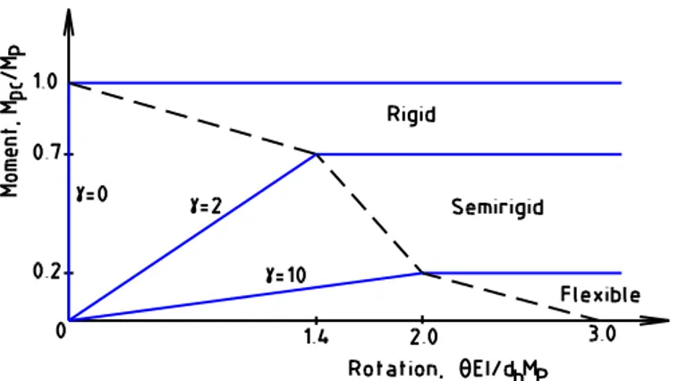
For the semi-rigid frames, we apply the moment – rotation relation for connections is used by F. Tin Loi et al. [9]. In this reference, the semi-rigid elastic-plastic properties in pure bending condition, namely initial stiffness and plastic moment capacity, are chosen according to the simple and elegant classification system proposed by Bjorhovde et al. [11]. The initial stiffness of each bilinear moment (Mpc) - rotation () relation is defined as:

Mpc =EI/db, (16) where  is a constant; db is the connecting beam depth. The graphical illustration of this behaviour is shown in Fig.2, where the ranges for rigid, semi-rigid and flexible behaviour are shown. Like in the reference [9], intermediate values of moment capacities for given stiffness were interpolated here in accordance with the dashed line shown Fig. 2. The example 2 and example 4 presented in this study are calculated in term of the values of s and of  reporting in the Table 1. Table1: Relation between s and 

s 0.1 0.2 0.3 0.4 0.5 0.6 0.7 0.8 0.9 1.0

 25.000 10.0000 6.2667 4.4000 3.2800 2.5333 2.0000 1.1667 0.5185 0.0000

Fig. 2: Idealized moment – rotation relation for connections

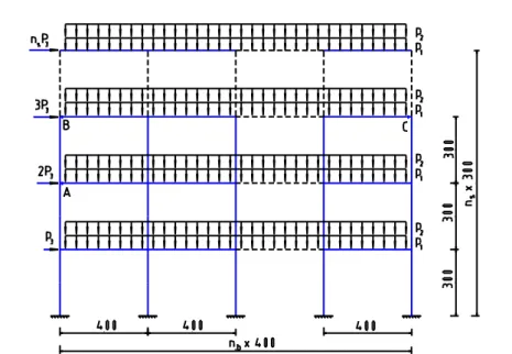
Example 1-Limit and shakedown analysis for rigid frame: A series of frames with different numbers of story (ns) and bay (nb) being already considered by Raffaele Casciaro et al. [25] are shown on the Fig. 3 (the units not mentioned). A constant story height hs = 300 and a constant bay length lb = 400 is assumed for simplicity and three loading cases are considered: two distributed vertical loads p1 and p2 and a seismic action defined as transversal force linearly increasing by P3 from the ground to the top floor (see Fig.3). Some mechanical properties are reported in Table 2, and the load domain is defined by: 9p110; 0p25; -500P3500.

The Table 3 presents the results of limit and shakedown analysis. According to the results given by CEPAO, with the case (*) (see Table 3, column 6), the incremental plasticity occurred, while the fatigue (the alternating plastic) is appeared in the case (**). The sections for which the fatigue occurs are A, B, C (see Fig.3) respectively for 46 frame, 59 frame and 610 frame.

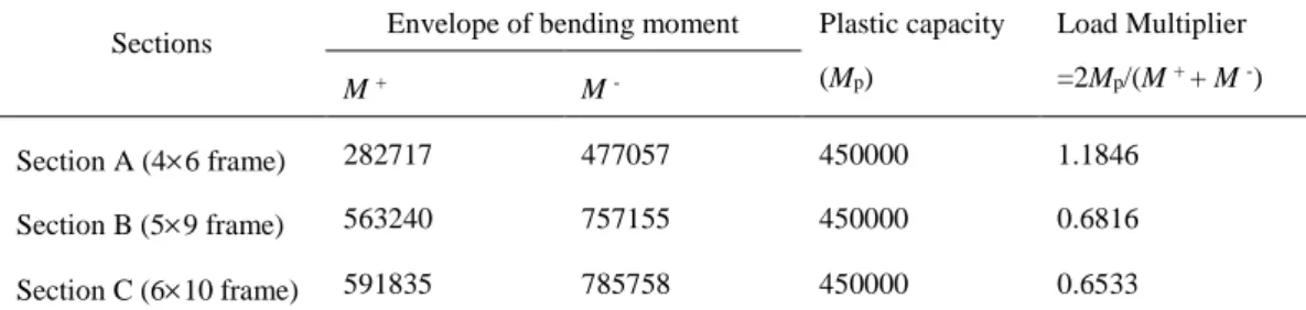
Discussion: The load multipliers obtained by [25] and by CEPAO are coincided in the case of limit analysis for all series of frames and in the case of shakedown analysis for 34 frame. While the differences are respectively: -10,5%, -6,4% and -6,5% for 46 frame, 59 frame and 610 frame in the shakedown analysis. The Table 4 presents the load multipliers in the case of shakedown analysis for 46, 59, 610 frame, with the following assumption: The alternating plastic occurs in the sections A, B, C with the envelope of bending moment calculated by the software SAP2000. As the load multipliers in the Table 4 are the upper bounds, the real load multipliers cannot exceed these values. The differences between the results obtains by CEPAO and the above-mentioned values is about from 3,5% to 6,4%, and those of ref. [25] are from 9,4% to 15,3%. It is useful to

denote that the differences of the value of the envelope of the bending moment between SAP2000 and CEPAO is due to the lumping of the uniformly distributed load at the central point and the two ends of each element in the CEPAO.

Table 2: Example 1 – Mechanical properties for the series of frames

Young modulus (E) Moment of inertia (I) Plastic capacity (MP)

Column 300000 540000 1800000

Beam 300000 67500 450000

Fig. 3: Example 1-geometry and loads for the series frames

Table3: Example1 – Load multiplier for limit and shakedown analysis calculated by ref. [25] and CEPAO

Type of frame (ns x nb)

Limit analysis Shakedown analysis Ref. [25] CEPAO Difference Ref. [25] CEPAO Difference 34 frame 2.4612 2.4612 0.0% 2.0134 2.0102(*) 0.0% 46 frame 1.8610 1.8610 0.0% 1.3993 1.2655 (**) -10.5% 59 frame 1.2000 1.2000 0.0% 0.7533 0.7076(**) -6.4% 610 frame 1.1532 1.1532 0.0% 0.7209 0.6771 (**) _-6.5%

Table 4: Example 1 –Load multipliers for the fatigues occurring in the section A, B, C using the envelope of bending moment calculated by SAP2000.

Sections Envelope of bending moment Plastic capacity (Mp) Load Multiplier =2Mp/(M + + M -) M + _M - Section A (46 frame) 282717 477057 450000 1.1846 Section B (59 frame) 563240 757155 450000 0.6816 Section C (610 frame) 591835 785758 450000 0.6533

Example 2-Limit and shakedown analysis for semi-rigid frames: These examples are already considered by F. Tin Loi et al. [9]. The aim of this study is to find the difference between shakedown and collapse limits for varying connection strengths with two following mechanical and geometric data (in tonne and metre units):

Fig. 4: Example 2 – Frame geometry and loading

Data a: The frame geometry and loading are shown in the Fig.4a, the properties of all elements are: E = 2.1107; I = 118.510-6; MP = 20; db = 0.3;

Data b: The frame geometry and loading are shown in the Fig.4b, with the following properties: for the column: E = 2.1107; I = 85.210-6; MP = 10; for the beams: E = 2.1107; I = 118.510-6; MP= 20; db = 0.3.

These two examples are analysed by CEPAO. The results are compared with those from F. Tin Loi et al. [9] and illustrated on the Table 5 and the Fig. 5a and 5b. With the data a, the alternating plasticity occurs in the shakedown analysis with s = 0.1 and 0.2.

Table5: Example 2 – Load Multipliers Type of analyse Connection strengths (s) 0.1 0.2 0.3 0.4 0.5 0.6 0.7 0.8 0.9 1.0 Example 2, data a Collapse by ref. [9]* _{3.70 4.01 4.36 4.67 5.05 5.22 5.43 5.60 5.81 6.02} 4.01 4.36 4.67 5.05 5.22 5.43 5.60 5.81 6.02 Collapse by CEPAO 3.67 4.00 4.33 4.67 5.00 5.20 5.40 5.60 5.80 6.00 4.00 4.33 4.67 5.00 5.20 5.40 5.60 5.80 6.00 Shakedown by ref. [9]* _{2.42 3.04 3.77 4.01 4.25 4.53 4.77 5.01 5.29 5.57} 3.04 3.77 4.01 4.25 4.53 4.77 5.01 5.29 5.57 Shakedown by CEPAO 2.54 3.28 3.78 4.03 4.28 4.54 4.81 5.06 5.30 5.56 3.28 3.78 4.03 4.28 4.54 4.81 5.06 5.30 5.56 Example 2, data b Collapse by ref. [9]* _{0.53 0.80 1.02 1.14 1.25 1.34 1.42 1.49 1.49 1.49} 0.80 1.02 1.14 1.25 1.34 1.42 1.49 1.49 1.49 Collapse by CEPAO 0.53 0.80 1.02 1.14 1.25 1.33 1.42 1.48 1.48 1.48 0.80 1.02 1.14 1.25 1.33 1.42 1.48 1.48 1.48 Shakedown by ref. [9]* _{0.50 0.71 0.91 1.00 1.12 1.18 1.25 1.31 1.35 1.35} 0.71 0.91 1.00 1.12 1.18 1.25 1.31 1.35 1.35 Shakedown by CEPAO 0.50 0.71 0.91 1.01 1.12 1.19 1.26 1.32 1.35 1.35 0.71 0.91 1.01 1.12 1.19 1.26 1.32 1.35 1.35

(*) We obtain these results by treating the figure in reference [9] (Fig. 6 and Fig. 8) in the case of pure bending hinges.

Fig.5: Example 2-Variation of load multiplier with connection strength (Tab. 5) a- data a; b- data b

Example 3– Elastic-plastic analysis with 2nd order for rigid frame: The purpose of this example is the determination the load multiplier under second order effect for the rigid frame shown in Fig. 6a.

a. The data is used by F. Tin Loi et al. [10], in ton and inch units: E = 1.3393104_{, H = 144; L = 90; 2P}

1 = P2 = 8.375; 2P3 = P4 = 0.402; members 1,2: I = 115.06; MP = 502.3; members 5, 6: I = 86.69; MP = 393.5; members 9, 10: I = 43.69; MP = 259.3; members 13, 14: I = 34.71; MP = 205.3; members 15, 16: I = 55.63; MP = 244.0; and other members: I = 122.34; MP = 428.0.

We observe a very good agreement between the value given by CEPAO (2.036) and the one by F. Tin Loi et al. [10] (2.037)

b. The data is analysed by S. Baset et al. [26], in kip and inch units: E = 3103; H = 144; L = 180; P1 = P2 = 30; 2P3 = P4 = 7.2; members 1,2,5,6,9,10,13,14, I = 344; MP = 2560; members 11,12,15,16: I = 891; MP = 3822; members 3, 4,7,8: I = 984; MP = 4204.

CEPAO provides a value of 2.123, while S. Baset et al. [26] give 2.079. The difference is 2.07%.

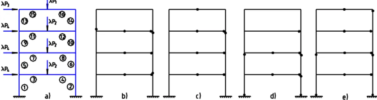
At Fig.6 b, c, d, e we compare the hinge dispositions in the frame given by CEPAO and other researchers [10, 26].

Fig. 6: Example 3 – Frame geometry and loading and hinge dispositions a- Frame geometry and loading; b, c, d, e - The hinge dispositions (b- Ref. [10], c

– CEPAO with data a, d – Ref. [26], e - CEPAO with data b)

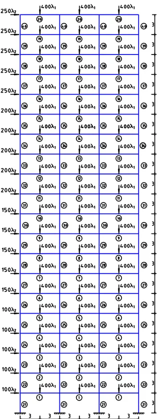
Example 4 – Analysis and optimization for large dimension semi-rigid frame by CEPAO: A twenty stories three bays semi-rigid frame with geometry and loading shown on the Fig.7 is analysed by CEPAO with the following studies: elastic analysis; first order elastic-plastic step by step analysis; elastic-plastic step by step analysis with second order effect; rigid-plastic analysis; shakedown analysis; optimization-limit; optimization-shakedown.

Concerning loading domain, for shakedown problems, two cases are considered: a) 011, 02 1 and b) -111, 021. For fixed or proportional loading obviously we must have: 1=2=;

For the optimal problem, forty different groups of elements are chosen as conception variables (Fig.7) and the adopted fixed load factor is  = 0.25. Here only the costs of semi-rigid connections are considered. In the optimal-shakedown problem, the results of the iterative process consisting of updating the inertias depending on the plastic capacity: Ik/Imax = (Mpk/Mpmax)1.4.

For the analysis problems, seven different groups of elements are considered (Table 6). The yield stress p = 23.5104 KN/m2.

Tables 7, 8 and Fig.8-11 present some results, in which KN and m units are used. Table 6: Example 4 – Profile used for analysis problems

Groups 1-5 6-10 11-15 16-20 21-25 26-30 31-35 36-40

Profile IPE550 IPE500 IPE450 IPE330 HE600A HE550A HE450A HE360

A

Table 7: Example 4 – Load Multipliers of analysis problems

Type of analyse Connection strengths (c) 0.1 0.2 0.3 0.4 0.5 0.6 0.7 0.8 0.9 1.0 0.2 0.3 0.4 0.5 0.6 0.7 0.8 0.9 1.0 Rigid-Plastic 0.080 0.121 0.162 0.202 0.244 0.284 0.324 0.360 0.396 0.432 0.121 0.162 0.202 0.244 0.284 0.324 0.360 0.396 0.432

Elastic-plastic first order 0.080 0.121 0.162 0.202 0.244 0.284 0.324 0.360 0.396 0.432

0.121 0.162 0.202 0.244 0.284 0.324 0.360 0.396 0.432

Elastic-plastic second order 0.053 0.088 0.127 0.167 0.205 0.241 0.280 0.316 0.354 0.392 0.088 0.113 0.1677 0.205 0.241 0.280 0.316 0.354 0.392

Shakedown, load domain (a) 0.065* _{0.110 0.145 0.181 0.217 0.253 0.288 0.324 0.359 0.394}

0.113 0.149 0.185 0.221 0.256 0.292 0.326 0.36 0.394

Shakedown, load domain (b)* _{0.037 0.070 0.096 0.134 0.166 0.198 0.229 0.260 0.290 0.320}

(*) alternating plastic occurs.

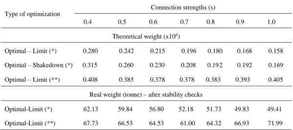
Table 8: Example 4 – Results of optimal problems

Type of optimization Connection strengths (s) 0.4 0.5 0.6 0.7 0.8 0.9 1.0 0.2 0.3 0.4 0.5 0.6 0.7 0.8 0.9 1.0 Theoretical weight (x106₎ Optimal – Limit (*) 0.280 0.242 0.215 0.196 0.180 0.168 0.158 0.673 0.453 0.343 0.280 0.242 0.215 0.196 0.180 0.168 0.158 Optimal – Shakedown (*) 0.315 0.260 0.230 0.208 0.192 0.192 0.169 0.790 0.495 0.368 0.315 0.260 0.230 0.208 0.192 0.192 0.169 Optimal – Limit (**) 0.408 0.385 0.378 0.378 0.383 0.393 0.405 Real weight (tonne) – after stability checks

Optimal-Limit (*) 62.13 59.84 56.80 52.18 51.73 49.83 49.41 Optimal-Limit (**) 67.73 66.53 64.53 61.00 64.32 66.93 71.99

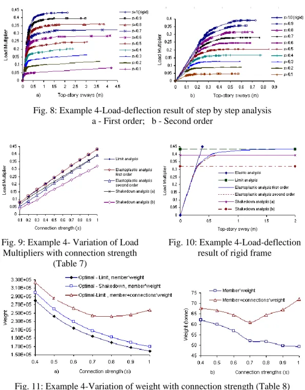
Fig. 8: Example 4-Load-deflection result of step by step analysis a - First order; b - Second order

Fig. 9: Example 4- Variation of Load Multipliers with connection strength

(Table 7)

Fig. 10: Example 4-Load-deflection result of rigid frame

Fig. 11: Example 4-Variation of weight with connection strength (Table 8) a -Theoretical weight; b-Real weight of optimal-limit

Remark: In the case of small connection strengths or symmetric loading (seismic

action in the example 1, horizontal load with load domain b of example 4), the load multipliers determined by shakedown analysis are the smallest (alternating

plastic occurs). In the design problems, the member plus connections costs is minimum at some values of connection strength (it is s=0.7 in the example 4, see Fig.11b), this value depends on the determination of the conventional length. On the other hand, the determination of the conventional length depends on a lot of parameters: the cost of material, the cost of fabrication (the cost of the labour), and these parameters may depend on country.

6 Conclusions

The CEPAO envisages the solutions for various loading conditions (proportional, repeated, alternative…), for various aspects (direct analysis and design, step-by-step analysis…) of the behaviour of the frames. An optimal solution may be found according for each practical case. CEPAO may be useful for the practice in civil engineering.

CEPAO is also an auto-controlled algorithm. Indeed, we can verify easily the results by using resident equivalent procedure. For example, limit analysis and analysis hinge-by-hinge must lead to the same limit load factor, while they are based on two dual methods (kinematical method and static method). After the optimal plastic design (or shakedown plastic design), the plastic analysis (or shakedown analysis) may be operated to reanalyse for checking if the limit load factor would be equal to 1 as theoretically expected. On the other hand, we can observe that the two modules of elastic analysis (by equilibrium-stiffness method) and limit analysis (by LP method) constitute the fundamental modules, which may lead to more complicated implementations, more realistic computations. The present extensions suggest that CEPAO constitutes a source for future implementations and researches in civil engineering practices.

In the near future, we hope to present the new version of the CEPAO for the space frameworks.

References

[1] Nguyen-Dang Hung, “CEPAO-an automatic program for rigid-plastic and elastic-plastic,

analysis and optimization of frame structure’’, Eng. Struc. Vol 6, 33-50, 1984.

[2] Nguyen-Dang Hung, Géry de Saxcé, “Analyse et dimensionnement plastique des

structures à barres dans les conditions de stabilité’’, Construction métallique, N°3,1981. [3] Nguyen-Dang Hung, “Sur la plasticité et le calcul des états limites par éléments finis’’,

[4] Nguyen-Dang Hung, “Sur l’utilisation du simplexe dans le CEPAO 82’’, Rapport interne n°133 du Laboratoire de Mécanique des Matériaux et de Stabilité des Constructions, l’Université de Liège, Belgique, 1983.

[5] Géry de Saxcé, L. M. Ayina ohandja, “Une méthode automatique de calcul de l’effet P -

Delta pour l’analyse pas - à - pas des ossatures planes’’, Construction métallique, n°3, 1985.

[6] Chen, W.F., Lui, E.M., “Stability design of steel frames’’, Boca Raton, FL: CRS Press,

1991.

[7] Chen, W. F, Yoshiaki G., Richard, J. Y., “Stability design of semi-rigid frames’’, John Wiley & sons, inc, 1996.

[8] Jaspart, J. P., “Etude de la semi - rigidité des nœuds poutre - colonne et son influence sur la résistance et la stabilité des ossatures en acier’’, Thèse de doctorat de l’Université de Liège, Belgique, 1991.

[9] F. Tin Loi, V. Vimonsatit, “Shakedown of frame with semi-rigid connections’’, Journal

of Structural Engineering, 119(6), 1694-1711, 1993.

[10] F. Tin Loi, V. Vimonsatit, “Nonlinear analysis of semi-rigid frames: a parametric complementarity approach’’, Engineering Structure, 18(2), 115-124, 1996.

[11] Bjorhovde, R., Colson, A., and Brozzetti, J., “Classification system for beam-to-column

connections’’, Journal of Structural Engineering, 116(11), 3059-3076, 1990.

[12] A. Colson, R. Bjorhovde, “Intérêt économiques des assemblages semi-rigides’’,

Construction métallique, n°2, 1992.

[13] Stéphane Guisse, “Quelle économie attendre de la mise en oeuvre de noeuds semi-rigides?’’, Construction métallique, n°3, 1993.

[14] Lei Xu and al., “Computer- Automated Design of Semi-rigid Steel Frameworks’’, Journal

of Structural Engineering, 119(6), 1741-1760, 1993.

[15] L. M. C. Simoes, “Optimization of frames with semi-rigid connections’’, Computers &

structures, 60(4), 531-539, 1996.

[16] M. S. Hayalioglu and al., “Minimum cost design of steel frames with semi-rigid connection and column bases via genetic optimization’’, Computers & structures, 83, 1849-1863, 2005.

[17] Eurocode 3- design of steel structures, Part 1.1: General rules and rules for buildings, European prestandard. ENV 1993-1-1, February 1992.

[18] J. M. Cabrero, E. Bayo, “Development of practical design methods for steel structures with semi-rigid connections’’, Engineering Structures, 27, 1125-1137, 2005.

[19] Hodge. P. G., “Plastic analysis of structures’’, McGraw Hill, New York, 1959.

[20] Neal. B. G., “The plastic method of structural analysis’’, Chapman & Hall, London, 1970.

[21] Massonnet, Ch., Save, M., “Calcul plastique des constructions’’, Volume 1, Nelissen, Belgique, 1976.

[22] Cohn, M. Z, Maier, G., “Engineering Plasticity by Mathematical Programming’’,

University of Waterloo, Canada, 1979.

[23] Milan Jirsek, Zdeněk P. Bažant, “Inelastic Analysis of Structure’’, John Wiley & Sons,

LTD, 2001.

[24] Nguyen-Dang Hung, Hoang-Van Long, “On the change of variables in the calculation plastic of structures by LP in the CEPAO program”, Internal Report of Division LTAS-Fracture Mechanics, University of Liège, 2006.

[25] Raffaele Casciaro, Giovanni Garcea, “An iterative method for shakedown analysis”, Computer methods in applied mechanics and engineering, 191, 5761-5792, 2002.

[26] S. Baset, D.E. Grierson and N.C.Lind, “Second – Order Collapse Load Analysis: a LP Approach’’, Solid Mechanics Division University of Waterloo, Canada, N°117, 1973.