présentée par
ZREIK Rawya
pour obtenir le grade de
DOCTEUR EN MATHÉMATIQUES APPLIQUÉES
Analyse statistique des réseaux et
applications aux Sciences Humaines
réalisée sous la direction de
Charles Bouveyron & Pierre Latouche
Soutenue publiquement le 30 novembre 2016 devant le jury composé de
M. Biernacki Christophe Université Lille 1 & Inria (Rapporteur)
M. Chiquet Julien AgroParisTech & Inra (Rapporteur)
Mme. Cottrell Marie Université Paris 1 (Examinateur)
Mme. Matias Catherine CNRS & Université Paris 6 (Examinateur)
M. Come Etienne IFSTTAR (Examinateur)
M. Velcin Julien Université Lyon 2 (Examinateur)
M. Lamassé Stéphane Université Paris 1 (Examinateur)
M. Bouveyron Charles Université Paris 5 (Directeur)
M. Latouche Pierre Université Paris 1 (Encadrant)
I would like to take this opportunity to thank the people with
whom I have worked for the last three years, who have made the
development of this thesis possible.
Charles and Pierre, thanks a lot for this chance that you gave me to
be in your team, for your support and thesis supervision.
I would especially like to thank my husband and family. Thank you
for being with me always, you have given me confidence and helped
me to advance.
Lastly, a big thanks to all members of the SAMM laboratory as well
as the MAP5 laboratory, especially Marie Cottrell and Jean-Marc
Bardet.
List of figures IX
List of tables XII
1 Introduction 1
1.1 Framework and contributions of the thesis . . . 1
1.2 Organization of the thesis . . . 4
1.2.1 The main Publications . . . 6
2 State of the art 9 2.1 Basics of the graph theory . . . 10
2.1.1 Types of graphs . . . 10
2.1.2 Encoding . . . 18
2.1.3 Indicators . . . 18
2.1.4 Proprieties of real networks . . . 20
2.2 Basic of clustering . . . 20
2.2.1 Partitional Clustering . . . 21
2.2.2 Hierarchical Clustering . . . 21
2.2.3 Mixture model clustering . . . 23
2.2.4 Graph clustering . . . 26
2.3 Clustering models for static graphs . . . 28
2.3.1 Community structure . . . 29
2.3.2 Cluster structures . . . 30
2.4 Clustering models for dynamic graphs . . . 35
2.4.1 Context and notations . . . 35
2.4.2 Dynamic mixed membership stochastic block model . . . 35
2.4.3 Dynamic stochastic block model . . . 37
2.5 Third-party models . . . 38 I
2.6.1 Variational inference algorithms . . . 47
2.6.2 Model selection criteria . . . 52
2.6.3 Bayesian information criterion . . . 54
2.7 Conclusion . . . 56
3 Dynamic random subgraph model 57 3.1 Introduction . . . 58
3.2 The dynamic random subgraph model . . . 60
3.2.1 Context and notations . . . 60
3.2.2 The model at each time t . . . 62
3.2.3 Modeling the evolution of random subgraphs . . . 63
3.2.4 Joint distribution of dRSM . . . 64
3.3 Estimation . . . 65
3.3.1 A variational framework . . . 66
3.3.2 A VEM algorithm for the dRSM model . . . 68
3.3.3 Optimization of ⇠ . . . 72
3.3.4 Model selection: choice of the number Q of latent groups 73 3.4 Numerical experiments and comparisons . . . 73
3.4.1 Experimental setup . . . 73
3.4.2 An introductory example . . . 74
3.4.3 Study of the evolution of the size on the network . . . 75
3.4.4 Choice of Q . . . 76
3.4.5 Comparison with the other stochastic models . . . 78
3.5 Conclusion . . . 83
4 Stochastic Topic Block Model 85 4.1 Introduction . . . 86
4.2 The model . . . 88
4.2.1 Context and notations . . . 88
4.2.2 Modeling the presence of edges . . . 89
4.2.3 Modeling the construction of documents . . . 90
4.2.4 Link with LDA and SBM . . . 92
4.3 Inference . . . 93
4.3.1 Variational decomposition . . . 93
4.3.2 Model decomposition . . . 94
4.3.3 Optimization . . . 94
4.3.4 Derivation of the lower bound ˜L (R(·); Z, ) . . . 96
4.3.5 Initialization strategy and model selection . . . 99
4.4 Numerical experiments . . . 102
4.4.1 Experimental setup . . . 102
4.4.2 Introductory example . . . 103
4.4.3 Model selection . . . 105
5.1 Applications of dRSM . . . 110
5.1.1 Maritime flows . . . 110
5.1.2 Application to the Enron network . . . 128
5.2 STBM applications . . . 133
5.2.1 Enron email network analysis . . . 134
5.2.2 Nips co-authorship network analysis . . . 139
5.3 Conclusion . . . 140
6 Conclusion and perspectives 143 6.1 Contributions of the thesis . . . 143
6.2 Perspectives . . . 144
6.2.1 Methodological perspectives . . . 144
6.2.2 Application perspectives . . . 145
Appendices 146
A The Forward-backward algorithm 147
1.1 Maritime network between 50 ports over the 4 years before and after the collapse of the USSR. The known subgraphs correspond to political systems in countries, indicated using colors. . . 3 1.2 Static network describing electronic communications (edges)
be-tween 148 Enron employees (nodes), where each node color corre-sponds to the status of employees in Enron in November 2001. . 5 2.1 An undirected network with 10 nodes (or vertices) and 15 edges
(or links). . . 11 2.2 An example for both directed and undirected networks with 20
nodes. . . 12 2.3 The metabolic network of bacteria Escherichia coli (Lacroix et al.,
2006). Nodes of the undirected network correspond to biochemical reactions, and two reactions are connected if a compound produced by the first one is a part of the second one (or vice-versa). . . . 13 2.4 Simulated data set of a dynamic network showing the evolution
of connections between 10 nodes for 4 different time-points. . . . 14 2.5 Dynamic network between 70 Enron employees for 4 months before
and after the bankruptcy of the company. The Enron data set, describes the exchange of emails among individuals who have worked for the Enron company. . . 15 2.6 Florentine business network describing the business ties between
16 Renaissance families. The vector of covariates for each node is provided. . . 16 2.7 An undirected network with 10 nodes and 13 edges having different
types, as indicated by their colors and line styles. . . 17
2.9 An example of the K-means clustering of the "iris" data set. This data contains the features of three differents species of flower. The results demonstrate that that Petal.Length and Petal.Width were similar among the same species but varied considerably between
different species. . . 22
2.10 An example of the dendrogram of the "iris" data set. This data contains the features of three differents species of flower. The results demonstrate that that Petal.Length and Petal.Width were similar among the same species but varied considerably between different species. . . 23
2.11 An example of the finite Gaussian mixture clustering fitted via EM algorithm of the "iris" data set. This data contains the features of three differents species of flower. The results demonstrate that that Petal.Length and Petal.Width were similar among the same species but varied considerably between different species. . . 25
2.12 An example of an undirected network with 40 nodes showing the structure of two partially isolated communities represented in red and green. . . 27
2.13 An example of the star cluster of an undirected graph with 20 nodes. . . 27
2.14 An example for the matrix of connection probabilities between clusters (⇧) in the SBM model. The network is made of 10 nodes split into K = 3 clusters (indicated by the colors). . . 31
2.15 Graphical representation of the stochastic block model. . . 32
2.16 Example of an RSM network. . . 34
2.17 The graphical model of a first-order Markov chain. . . 38
2.18 Graphical model for state space model represents sequential data using a Markov chain of latent variables. . . 39
2.19 Actual (solid red lines) and estimated (solid black lines) values of the states of xnand the 2 standard error deviations( green dotted lines ). . . 43
2.20 Graphical representation of the LDA model. . . 45
3.1 Connections between a subset of 26 ports (from October 1890 to October 2008). Data extracted from Lloyd’s list. The known sub-graphs correspond to geographical regions (continents) indicated using colors. . . 61
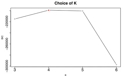
the colors). According to the dRSM model, the directed edges between the nodes can be of different types (C = 2 types are considered here). Given the clusters, the presence of an edge depends on the connection probabilities between clusters (⇧). . . 63 3.3 Graphical representation of the dRSM model. . . 65 3.4 Choice of Q by model selection with BIC for a simulated network.
The actual value for Q is 4. . . 75 3.5 Evolution of the bound ˜L for Q = 4. . . 76 3.6 Actual (dashed red lines) and estimated (solid black lines) values
of the group proportions for the simulated example (Q = 4 groups and S = 2 subgraphs). . . 77 3.7 ARI values depending on the size N of the networks in the binary
case (left) and categorical (right). . . 79 3.8 Criterion and ARI values over 50 networks generated. . . 80 4.1 A sample network made of 3 “communities” where one of the
communities is made of two topic-specific groups. The left panel only shows the observed (binary) edges in the network. The center panel shows the network with only the partition of edges into 3 topics (edge colors indicate the majority topics of texts). The right panel shows the network with the clustering of its nodes (vertex colors indicate the groups) and the majority topic of the edges. The latter visualization allows to see the topic-conditional structure of one of the three communities. . . 86 4.2 Graphical representation of the stochastic topic block model. . . 92 4.3 Networks sampled according to the three simulation scenarios A,
B and C. See text for details. . . 102 4.4 Clustering result for the introductory example (scenario C). See
text for details. . . 104 4.5 Clustering result for the introductory example (scenario C). See
text for details. . . 104 4.6 Introductory example: summary of connexion probabilities
be-tween groups (⇡, edge widths), group proportions (⇢, node sizes) and most probable topics for group interactions (edge colors). . . 105 5.1 The given partition of the 286 nodes (ports) into 4 subgraphs. . . 112 5.2 Adjacency matrix of the maritime network organized by subgraph
(basin) in 1890 (left) and 2008 (right). . . 112 5.3 BIC values according to the number K of groups for the maritime
network. . . 113 5.4 Terms ⇧1
kl of the tensor matrix ⇧ estimated using the VEM
algorithm. . . 114 5.5 Evolution of the proportions of the K = 7 latent clusters. . . 115
5.8 World maritime traffic. . . 118 5.9 Inter-subgraph maritime flows. . . 119 5.10 BIC values according to the number K of groups for the maritime
network. The actual value for K is 9. . . 120 5.11 Terms ⇡1
klof the tensor matrix ⇡ estimated using the VEM algorithm.121
5.12 The proportions of the latent clusters 1 and 9. . . 122 5.13 Evolution of the proportions of the K = 9 latent clusters . . . 123 5.14 Summary of connection probabilities between groups. . . 124 5.15 The partition of ports into 9 groups (colors) during 2 different
years (1990-1991). . . 125 5.16 Cluster geography during the 4 years before and after USSR
collapse for clusters 3,6 and 4,5. . . 126 5.17 Cluster evolutions in fonction of its ratio of weights. . . 127 5.18 Frequency of messages between Enron employees between
Septem-ber 1st and DecemSeptem-ber 31th, 2001. . . 128 5.19 Proportions of the K = 4 clusters, at each time. Subgraph 1
(Managers), left figure; subgraph 2 (employees), middle figure; subraph 3 (other), right figure. . . 130 5.20 Clustering result with STBM on the Enron data set (Sept.-Dec.
2001). . . 131 5.21 Most specific words for the 5 found topics with STBM on the
Enron data set. . . 132 5.22 Enron data set: summary of connexion probabilities between
groups (⇡, edge widths), group proportions (⇢, node sizes) and most probable topics for group interactions (edge colors). . . 132 5.27 Model selection for STBM on the Enron data set. . . 134 5.28 Reorganized adjacency matrix according to groups for STBM on
the Enron data set. . . 134 5.29 Specificity of a selection of words regarding the 5 found topics by
STBM on the Enron data set. . . 135 5.30 Estimated matrix ⇡ by STBM on the Nips co-authorship network. 136 5.31 Reorganized adjacency matrix according to groups for STBM on
the Nips co-authorship network. . . 137 5.32 Specificity of a selection of words regarding the 5 found topics by
STBM on the Nips co-authorship network. . . 138 5.23 Clustering results with SBM (left) and STBM (right) on the
Enron data set. The selected number of groups for SBM is Q = 8 whereas STBM selects 10 groups and 5 topics. . . 141 5.24 Clustering result with STBM on the Nips co-authorship network. 141 5.25 Nips co-authorship network: summary of connexion probabilities
between groups (⇡, edge widths), group proportions (⇢, node sizes) and most probable topics for group interactions (edge colors). . . 142
2.1 The main six words associated with each topic, as found by the LDA methodology. . . 47 2.2 Matrix of topic proportions for each document. . . 47 3.1 Summary of the notations used in the chapter. . . 66 3.2 Parameter values for the five types of graphs used in the
ex-periments. In scenario 0, the networks are drawn without an explicit temporal dependance whereas, in the other scenarios, the temporal dependance is generated through a state space model (ssm). . . 74 3.3 Actual (left) and estimated (right) values for the terms ⇧1
qlof the
tensor matrix ⇧. See text for details. . . 77 3.4 Actual (left) and estimated (right) values for the matrix ⇧c
ql with
c2 (0, 1, 2) ( from top to bottom). . . 78 3.5 The average execution time required by the VEM algorithm
de-pending on the size N of the network, in the binary case (left) and the categorical case (right) for T = 10. . . 79 3.6 Clustering results for the four studied methods on networks
simu-lated according to the five scenarios. The actual number Q = 4 of groups has been provided to each method here. Average ARI values are reported (with standard deviations) and results are averaged on 20 networks for each scenario. . . 81 3.7 Clustering results for the four studied methods on networks
sim-ulated according to the five scenarios. Average ARI values are reported (with standard deviations) as well as the selected number Qof latent groups. Results are averaged on 20 networks for each scenario. . . 82
4.1 Parameter values for the three simulation scenarios (see text for details). . . 103 4.2 Percentage of selections by ICL for each STBM model (Q, K) on
50 simulated networks of each of three scenarios. Highlighted rows and columns correspond to the actual values for Q and K. . . 106 4.3 Clustering results for the SBM, LDA and STBM on 20 networks
simulated according to the three scenarios. Average ARI values are reported with standard deviations for both node and edge cluster-ing. The “Easy” situation corresponds to the simulation situation describes in Table 4.1. In the “Hard 1” situation, the communities are very few differentiated (⇡qq = 0.25and ⇡q6=r= 0.2, except for
scenario B). The “Hard 2” situation finally corresponds to a setup where 40% of message words are sampled in different topics than the actual topic. . . 107 5.1 Time points considered in the maritime network. . . 111 5.2 The time periods considering for the analysis of e-mail exchanges
in the Enron company . . . 129 5.3 Terms ⇧kl1 of the matrix ⇧ estimated using the VEM algorithm 130
Summary of the notations used in this thesis Notations Description
G Presents a graph .
X Adjacency matrix, presenting either binary or categorical or textual edges between nodes.
Z Binary matrix, pinpointing each node and its cluster. N Number of vertices in the network or total number of words. L Number of links in the graph.
Q Number of latent clusters.
K Number of latent topics.
S Number of subgraphs.
C Number of edge types.
T Number of time points.
D Number of documents.
V Representing the total number of vocabulary in the full set of documents.
W Sequence of whole words on D document and Wd
n is the nth word
in the document d.
⇧ Describes the probabilities of connection between clusters, and ⇧c ql
is the probability of having an edge of type c between vertices of clusters q and l.
INTRODUCTION
Over the last two decades, network structure analysis has experienced rapid growth with its construction and its intervention in many fields, such as: com-munication networks, financial transaction networks, gene regulatory networks, disease transmission networks, mobile telephone networks. Social networks are now commonly used to represent the interactions between groups of people; for instance, ourselves, our professional colleagues, our friends and family, are often part of online networks, such as Facebook, Twitter, email.
Since Moreno’s original work on the network in 1934, research on the de-velopment of network structure has increased, and is still much debated, and over time, there has been an unprecedented rise in the amount of network data available.
1.1 Framework and contributions of the thesis
In a network, many factors can exert influence or make analyses easier to understand. Among these, we find two important ones: the time factor, and the network context. The former involves the evolution of connections between nodes over time. The network context can then be characterized by different types of information such as text messages (email, tweets, Facebook, posts, etc.) exchanged between nodes, categorical information on the nodes (age, gender, hobbies, status, etc.), interaction frequencies (e.g., number of emails sent or comments posted), and so on. Taking into consideration these factors can lead to the capture of increasingly complex and hidden information from the data.
The aim of this thesis is to define new models for graphs which take into consideration the two factors mentioned above, in order to develop the analysis of network structure and allow extraction of the hidden information from the data. These models aim at clustering the vertices of a network depending on their
connection profiles and network structures, which are either static or dynamically evolving. The starting point of this work is the stochastic block model, or SBM. This is a mixture model for graphs which was originally developed in social sciences. It assumes that the vertices of a network are spread over different classes, so that the probability of an edge between two vertices only depends on the classes they belong to. Despite the good performance of the clustering methods associated with this model on static networks, they are known to underperform when trying to take into consideration the network context for static networks, and also dealing with dynamic networks.
In this thesis, we intend to underline the problems which arise when using the SBM model. Therefore, we will offer solutions regarding the network structure analysis for different situations, either static or dynamic, and in various contexts. Thus, we undertake, on the one hand, defining a new model based on SBM to deepen the understanding of the network structure of dynamic networks. On the other hand, we look to understand the topology of the network, using both the connectivity between nodes and the context. To this end, we have three principal contributions, which are as follows.
In the first contribution, we propose a new random graph model, where we focus on modeling dynamic networks when taking into consideration time and the type of edges, which can be either categorical or binary. In this context, we try to discover the hidden characteristics and properties that explain a network over time, where a decomposition of the networks into subgraph is given. Once we have observed a categorical edge structure, we essentially treat the evolution of connections between nodes into subgraphs over time for the dynamic network. The subgraphs are assumed to be made of latent clusters which have to be inferred from the data in practice. The vertices are then connected with a probability depending only on the subgraphs whereas the edge type is assumed to be sampled conditionaly on the latent groups. Figure 1.1 illustrates an example of a dynamic network of a maritime network between 50 ports over the 4 years before and after the collapse of the Union of Soviet Socialist Republics (USSR). This example shows a real application of our methodology where the known subgraphs correspond to political systems in countries. Application of the proposed model allows us to:
1. Discover the network structure over time, capturing the evolution of con-nections between nodes over time from both the network’s graph and the categories of edges.
2. Detect communities and their behavior from binary or categorical interac-tions over time, depending on each of the subgraphs.
3. Find the probability of connections between communities of nodes present in the network.
4. Predict the edges from new nodes, based on types of intersections and their subgraphs.
1987 1989
1992 1994
Figure 1.1: Maritime network between 50 ports over the 4 years before and after the collapse of the USSR. The known subgraphs correspond to political systems in countries, indicated using colors.
In our second contribution, we propose a new model to address the prob-lem of finding topically meaningful clusters, by leveraging both links between individuals and text content shared between them in the static network. To this end, we are primarily concerned with accomplishing two tasks. The first one is to examine texts from social networks. The second one is to improve the understanding of the node’s identities, by incorporating network context into network analysis algorithms, and by analyzing both the context and the graph. In this model, we can cluster or categorize identities of nodes according to “metadata” attached to these nodes. For example, this includes text messages (from tweets, Facebook, posts, etc.), interaction frequencies (emails), and more. Figure 1.2 illustrates a real static network to which we can apply our methodol-ogy. This network describes electronic communications between 148 employees at the famous Enron1company. Application of this second new model allows us
to:
1. Discover network structure from both the network graph and context. For example, finding social network communities characterized both by link patterns and textual discourse.
2. Detect communities from textual interaction, such as emails and comments, etc.
3. Predict the edges to/from new nodes based only on textual data. For example: emails, newly written academic papers, etc.
4. Treat a graph as information flow between individuals and find sets of topics which summarize the subjects of network by studying this information. Finally, the last contribution is to validate the performance of our new models by applying each one to several real data sets. To this end, on the one hand, we applied the dRSM model to two real world networks: the first one, describes the electronic communications between employees in the Enron company. The second one describes the maritime flows in the word. On the other hand, we applied STBM to the Enron email and the Nips co-authorship networks
1.2 Organization of the thesis
The first chapter of the thesis describes the current state-of-the-art in this domain, from which our new results come. Some general notation is given, and the most well-known clustering methods for network analysis are reviewed. These methods are mainly focused on statistical models, along with other models for inference, such as the expectation maximization (EM) algorithm and the variational EM algorithm. We also focus on some model selection criteria to
November 2001
● ● ● ● ● ● CEO, presidents Vice−presidents, directors Managers, managing directors TradersEmployees Unknowns
Figure 1.2: Static network describing electronic communications (edges) between 148 Enron employees (nodes), where each node color corresponds to the status of employees in Enron in November 2001.
estimate the number of classes from the data. Lastly, we focus on tools that we can integrate into the network, such as state space models (SSM) and latent dirichlet allocation (LDA). Several applications are presented in order to explain and clarify the model.
The second chapter presents our new model to analyze dynamic networks, which we call the dynamic random subgraph model (dRSM). This model is an extension of the random subgraph model (RSM) which was recently defined in order to deal with dynamic networks, using a state space model to characterize cluster proportions. A variational expectation maximization, or VEM, algorithm is proposed to approximate the posterior distribution over the model parameters and latent variables, which leads to a new state space model.
The third chapter defines the stochastic topic block model (STBM), which is a new model built to analyze networks with textual edges. STBMs aim to discover meaningful clusters of vertices that are coherent from both the network interaction and text content points of view. A classification variational expectation maximization (C-VEM) algorithm is proposed to perform inference. Lastly, in the fourth chapter, we apply the two new models to real data sets. First, we show the capacity of dRSM to capture network dynamics, in order to uncover the evolution of clusters over time, in two different data sets. The first data presents a social network describing the electronic communications between employees. The second one is a geographical network which describes the maritime flows in the word. Secondly, we apply STBM to two different social networks: the Enron email and the Nips co-authorship networks, showing the ability of our methodology to detect communities, according to links and texts between nodes.
1.2.1 The main Publications
The main results of this thesis have been published in 3 articles (3 published), as well as one book chapter, which are:
- (Zreik et al., 2015): R. Zreik, P. Latouche, and C. Bouveyron. Classification automatique de réseaux dynamiques avec sous-graphes: étude du scandale enron. Journal de la Société Française de Statistique, 156(3):166–191, 2015.
- (Latouche et al., 2015): P. Latouche, R. Zreik, and C. Bouveyron. Cluster identification in maritime flows with stochastic methods. Maritime Networks: Spatial Structures and Time Dynamics, Routledge, 2015.
- (Zreik et al., 2016): R. Zreik, P. Latouche, and C. Bouveyron. The dynamic random subgraph model for the clustering of evolving networks. Computational Statistics, in press, 2016.
- (Bouveyron et al., 2016): C. Bouveyron, P. Latouche and R. Zreik. The stochastic topic block model for the clustering of vertices in networks with textual
STATE OF THE ART
Contents
2.1 Basics of the graph theory . . . 10 2.1.1 Types of graphs . . . 10 2.1.2 Encoding . . . 18 2.1.3 Indicators . . . 18 2.1.4 Proprieties of real networks . . . 20 2.2 Basic of clustering . . . 20 2.2.1 Partitional Clustering . . . 21 2.2.2 Hierarchical Clustering . . . 21 2.2.3 Mixture model clustering . . . 23 2.2.4 Graph clustering . . . 26 2.3 Clustering models for static graphs . . . 28 2.3.1 Community structure . . . 29 2.3.2 Cluster structures . . . 30 Stochastic block model . . . 30 Mixed membership stochastic block model . . . 33 Random subgraph model . . . 33 2.4 Clustering models for dynamic graphs . . . 35 2.4.1 Context and notations . . . 35
2.4.2 Dynamic mixed membership stochastic block model 35
2.4.3 Dynamic stochastic block model . . . 37 2.5 Third-party models . . . 38 2.5.1 State space model . . . 38 SSM Example . . . 42 2.5.2 Latent Dirichlet allocation model . . . 44
LDA example . . . 46 2.6 Inference algorithms and model selection . . . 47 2.6.1 Variational inference algorithms . . . 47 Variational EM algorithm . . . 50 Variational Bayes EM algorithm . . . 51 2.6.2 Model selection criteria . . . 52 Akaike’s information criterion . . . 53 2.6.3 Bayesian information criterion . . . 54 Integrated classification likelihood criterion . . . 55 2.7 Conclusion . . . 56
This chapter is the introduction to several state of the art methods dealt with in this thesis. Section 2.1 introduces the general concept wherein the theory and general notations are provided. Section 2.3 defines some recent statistical methods for the modeling of static networks with an emphasis on the clustering of vertices and the estimation of model parameters. Then, in Section 2.4, are included models capable of handling dynamic networks. Section 2.5 defines tools that we later integrate to network models, to improve its analysis. In particular, we present tools to find the latent topics among documents, and tools to capture the evolution of connections between observations over time. Lastly, Section 2.6 illustrates, on the one hand, some variational techniques which lie at the core of the main inference strategies for networks developed in this thesis. On the other hand, we introduce some criteria to estimate the number of classes in networks.
2.1 Basics of the graph theory
The development of scientific studies has encouraged the rising need for network analysis in all fields, for instance in biology, history, geography, social media, etc. Since 1730, when Leonhard Euler published his paper on the problem of the Seven Bridges of Köningsberg (Biggs et al., 1976), the graph theory has received strong attention from mathematical researchers, computer scientists, physicists, and sociologists. This research field allows the modeling of complex systems by characterizing pairwise interactions between objects of interest.
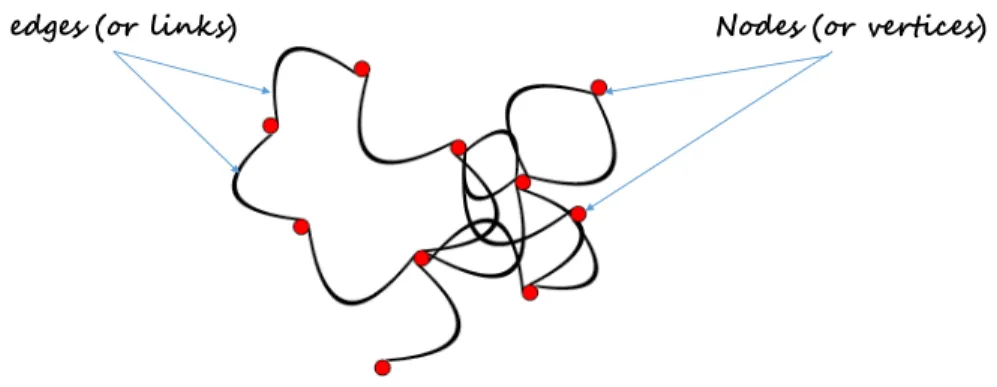
A graph is simply a collection of connected objects. We refer to these objects as “vertices” or “nodes”. A node might be an individual, a computer, a site or even some geographical location. The connections between vertices are then defined by “edges” also called “links” (see Figure 2.1). In terms of vocabulary, the terms “network” and “graph” can be used as synonyms. In practice, the term “graph” is mainly used when characterizing the mathematical structure while “network” usually refers to the graph and all information available on it.
2.1.1 Types of graphs
Depending on the types of pairwise information provided in a data set, various types of graphs can be considered for modeling. The types of graph depend essentially on the types of edges and the presence of data on the edges.
edges (or links) Nodes (or vertices)
Figure 2.1: An undirected network with 10 nodes (or vertices) and 15 edges (or links).
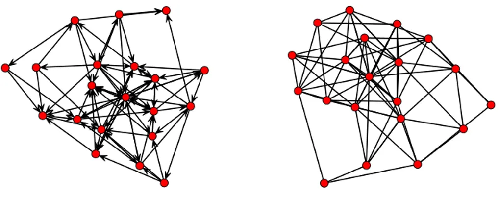
Undirected / directed If the connections between vertices are not oriented, i.e. if vertex i is linked to j, then j is linked to i, the graph is undirected. Conversely, if relationships are oriented, then the graph is directed. For instance, in friendships networks, characterizing the recorded friendship links of students in a school, it is a common practice to find students naming others as friends with no reciprocity. Examples of undirected networks can be found for instance in biology with the use of protein networks to describe the binding of proteins. Two proteins are linked if their are known to bind in the cells. Figure 2.2 presents an example of both directed and undirected networks.
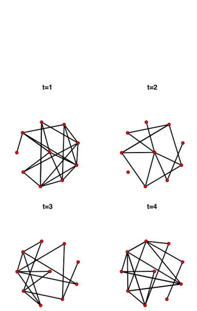
Static / dynamic If the connections between vertices are fixed over time, the data can be modeled as a static graph with fixed nodes and edges. An example of a static network is provided in Figure 2.3. However, as we shall see in Chapter 3, most networks used in real applications are dynamic with nodes and/or edges evolving over time. Nodes can appear or vanish. For instance, in a network characterizing the hyperlinks between websites, it is common to have new websites being created or closed. In Figures 2.4 and 2.5 the vertex set is fixed. However, the presence or absence of links between vertices change over time.
Figure 2.2: An example for both directed and undirected networks with 20 nodes.
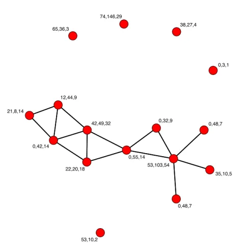
Type of edges When modeling a real data set as an network, the starting point is usually to describe the presence or absence of pairwise relationships between vertices. In that case, edges can be characterized as binary variables with 1 indicating the existence of an edge, and 0 otherwise. Then, information on the edges can also be available. Indeed, edges can be attached to values in a given set. This is the case for instance when considering similarity measures or distances between species in a network. Graphs with binary edges are called binary graphs while they are called valued or weighted graphs if they are made of valued edges. If the graph allows several connections between each pair of vertices, it is called a multigraph. Note that a multigraph is a special case of valued graph where all edges between a pair of vertices are aggregated to a unique edge with value counting the original number of edges between the pair. Other types of variables can be associated to the edges such as categorical variables for instance. They are commonly used to give the type of relationship between nodes. In the social framework, real networks are often made of edges representing the so called social interactions. These interactions usually take the form of documents such as articles, emails, text messages, posts, etc. In this scenario, an edge is associated to a collection of texts made of words, which are recorded. We call the graphs made out of these data sets textual graphs. Covariates Given a network, extra information on the vertices and / or edges can be available. For instance, Figure 2.7 is made out of nodes for which groups indicated by colors are given. The groups can be characterized by categorial variables on the vertices. Other types of covariate information can be provided with continuous variables for instance. Thus, the Florentine business network given in Figure 2.6 represents the business binary relations among 16 Renaissance families. Three quantitative node covariates are given for each family, namely the family’s net wealth in 1472, the family’s number of seats on the civic councils held between 1282 and 1344, and the family’s total number of business and
Figure 2.3: The metabolic network of bacteria Escherichia coli (Lacroix et al., 2006). Nodes of the undirected network correspond to biochemical reactions, and two reactions are connected if a compound produced by the first one is a part of the second one (or vice-versa).
t=1 t=2
t=3 t=4
Figure 2.4: Simulated data set of a dynamic network showing the evolution of connections between 10 nodes for 4 different time-points.
October 2001 December 2001
January 2002 February 2002
Figure 2.5: Dynamic network between 70 Enron employees for 4 months before and after the bankruptcy of the company. The Enron data set, describes the exchange of emails among individuals who have worked for the Enron company.
53,10,2 65,36,3 0,55,14 12,44,9 22,20,18 0,32,9 21,8,14 0,42,14 53,103,54 0,48,7 42,49,32 0,3,1 38,27,4 35,10,5 74,146,29 0,48,7
Figure 2.6: Florentine business network describing the business ties between 16 Renaissance families. The vector of covariates for each node is provided. marriage ties in the entire data set. In some cases, covariate information on the edges is also provided.
Hypergraphs To conclude, let us emphasize that graphs can be extended by allowing edges to connect not exclusively pairs of nodes, but any number of vertices. The corresponding mathematical object is called hypergraph in the literature. Hypergraphs are for instance of interest when describing all the authors of scientific papers. Rather than considering a series of edges to model the pairwise relationships between all the authors of a paper, a unique hyperedge can be taken into account, connecting all the authors.
Figure 2.7: An undirected network with 10 nodes and 13 edges having different types, as indicated by their colors and line styles.
2.1.2 Encoding
Many approaches exist to encode graphs as data structures, the two most common ones being as a list of edges and as an adjacency matrix. Other techniques include the use of incidence matrices or successor lists. Note that the latter are essentially only used in operational research, to deal with flows, and are outside the scope of this thesis.
Let us consider a graph G, characterized by a set of vertices denoted by V (G) with N nodes, as well as a set of edges denoted by E(G). The edge list coding simply consists in recording all the edges in E(G) as a list, each element being an edge of E(G). The key advantage of such approach is that only the presence of edges is recorded. The non edges are not taken into account. Conversely, an adjacency matrix stores information for every pair of nodes. This N ⇥ N matrix, denoted by X here, satisfies
Xij=
⇢
1if node i connects to node j 0otherwise.
As an illustration, the network with N = 9 nodes, provided in Figure 2.8, can be encoded with the following adjacency matrix and edge list {X13, X14, X21, X34,
X38, X48, X59, X65, X78, X79, X84}. X = 2 6 6 6 6 6 6 6 6 6 6 6 6 4 0 0 1 1 0 0 0 0 0 1 0 0 0 0 0 0 0 0 0 0 0 1 0 0 0 1 0 0 0 0 0 0 0 0 1 0 0 0 0 0 0 0 0 0 1 0 0 0 0 1 0 0 0 0 0 0 0 0 0 0 0 1 1 0 0 0 1 0 0 0 0 0 0 0 0 0 0 0 0 0 0 3 7 7 7 7 7 7 7 7 7 7 7 7 5
Note that Xii = 0,8i and therefore the network does not have any self-loops,
that is the connection of node to itself. The adjacency matrix is made of 9 ones corresponding to 11 edges.
2.1.3 Indicators
Several indicators are commonly used to characterize networks. They are also of interest when comparing the global structures of networks.
• number of edges : in this thesis, the number of edges is denoted by m. In the case of an undirected network, it is given by m = 0.5PN
i,jXij and
simply m =PN
1 2 3 4 5 6 7 8 9 X13 X14 X21 X34 X38 X48 X59 X65 X78 X79 X84
Figure 2.8: An example for a directed network with 9 nodes and 11 edges, in which we label each edge with the component of the adjacency matrix X.
• degree of a vertex : two vertices are called adjacent if they share a common edge, therefore the neighborhood N(v) of a vertex v in a graph G is the set of vertices adjacent to v. Furthermore, we can characterize each node v by its degree deg(v) which is the number of edges to which v is connected. In other words, the degree of a vertex is the total number of vertices adjacent to the vertex, deg(v) = |N(v)|. It can be easily derived from the adjacency matrix X, deg(v) = N X i=1 Xiv+ N X i=1 Xvi,
in the directed case,
deg(v) =
N
X
i=1
Xiv,
in the case of an undirected network.
• density of a network : the density of a network can easily be obtained from the number m of edges present. It is given by
(G) = m L,
where L is the number of potential connections, depending on the number N of vertices and the type of network considered. Thus, in the case of networks with self-loop, we have L is given by:
L = ⇢
N2 if directed
N (N + 1)/2otherwise, and if the network has no self loop,
L = ⇢
N (N 1)if directed N (N 1)/2otherwise.
• Clustering coefficient: the clustering coefficient (Cc) of a vertex represents the probability that the neighbors of a vertex are also connected to each other. That is to say, the clustering coefficient is the probability for two vertices i and j to connect to a third vertex k, such as:
Cc = p(XijXikXki= 1|XikXjk= 1)
= number of pairs of neighbors connected by edges number of pairs of neighbors .
2.1.4 Proprieties of real networks
Interestingly, most real networks have been shown to share some properties (Albert et al., 1999; Broder et al., 2000; Dorogovtsev et al., 2000) that we briefly
recall in the following.
• Sparsity: The number of edges is linear in the number of vertices. • Existence of a giant component: Connected subgraph that contains a
majority of the vertices.
• Heterogeneity: A few vertices have a lot of connections while most of the vertices have very few links. The degrees of the vertices are sometimes characterized using a scale free distribution (for instance see Barabasi and Albert, 1999).
• Preferential attachment: New vertices can associate to any vertices, but “prefer” to associate to vertices which already have many connections. • Small world: The shortest path from one vertex to another is generally
rather small.
2.2 Basic of clustering
Clustering and classification are both fundamental tasks in Data Science. Classi-fication is used mostly as a supervised classiClassi-fication method and clustering for unsupervised classification when the class information is missing. The clustering is the process which seeks to divide a data set into homogeneous groups. This process is based on information which is found in the data that describes the objects and their relationship. The goal is to discover as many similarities as possible between the members within a group and as many dissimilarity as possible between groups. More specifically, cluster analysis tries to identify homogeneous groups in a given data set. For example, in biology, cluster analysis can be used for clustering proteins on the based on their characteristics.
In this section, we will focus on the unsupervised classification and we consider three simple and important techniques to introduce the concept of cluster analysis, namely, hierarchical clustering (based on the Agglomerative and divisive algorithms), partitional clustering ( based on the K-Means algorithm) and mixture model clustering.
2.2.1 Partitional Clustering
The best examples of this family of clustering are K-means and K-medoids (also known as partition around medoids (PAM)). The K-means clustering was proposed by MacQueen et al. (1967) and intends to partition N objects into Q clusters in which each object belongs to the cluster with the nearest mean. Here, we have supposed that the number Q of clusters is fixed. In Section 2.6.1, we will see how Q can be estimated from the data. Let us consider a continuous data set {x1, x2, . . . , xN} consisting of N observations of a random d-dimensional
vector. Our goal is to partition the data into Q disjoint clusters {P1,· · · , PQ}
such that Pr\ Pl = ;, where the prototype of any cluster q 2 {1, . . . , Q} is
often a centroid, i.e the average (mean) of all points in the cluster noted ⌘q.
When the data has categorical variable, the prototype is often a medoid i.e, the most representative point of a cluster. For each point {xn}1,...,N, we introduce
a corresponding indicator variable Znq such as it equals to 1 if xn belongs to
cluster q and 0 otherwise. Then, the objective of K-means clustering is to find values of the {Z} and {⌘} which minimize the sum of squares of the distances between each point and its closest prototype (⌘):
J = N X i=1 Q X q=1 Ziqkxi ⌘qk2.
To start this algorithm (Algorithm 1), we select Q random points as cluster centers. Then, in the first step, we minimize J with respect to Z while the set {⌘1, . . . , ⌘Q} is fixed. The corresponding computational cost is O(QNd). In
the second step, J is minimized with respect to the set of {⌘}q=1,...,Q keeping
Z fixed. The time required here for calculating the centroids is O(Nd). We repeat the steps 1 and 2 until the same points are assigned to each cluster in two consecutive rounds. We note that, in these two steps, we calculate the centroid or mean of all objects in each cluster and assign objects to their closest cluster center according to the Euclidean distance function. An example of the clustering result of K-means is shown in Figure 2.9.
2.2.2 Hierarchical Clustering
Hierarchical clustering involves creating clusters that have a predetermined ordering from top to bottom, i.e. a tree of clusters, also known as a dendrogram (see Figure 2.10). Hierarchical clustering methods can be categorized into agglomerative (bottom-up) and divisive (top-down) (Jain and Dubes, 1988; Kaufman and Rousseeuw, 1990). In order to decide which clusters should be combined (for agglomerative), or whether a cluster should be split (for divisive), a measure of dissimilarity between sets of observations is required. In most methods of hierarchical clustering, this is achieved by the use of an appropriate metric (a distance measure between pairs of observations). Distances between objects can be visualized in many simple yet clear ways. For example, the initial
Algorithm 1: The basic procedure of K-means.
INITIALIZATION
Step 0 : Random initialization of Q clusters (⌘0)
OPTIMIZATION
⌘old
q ⌘qnew, 8q
repeat
step 1 : Assign each data object to its nearest cluster ⌘q, such as
for i in 1: N do
q= argminlkxi ⌘loldk2
Ziq 1
Zil 0, 8 l 6= q
step 2 : Update the centroid of each changed cluster until there is no change in any cluster
● ● ● ● ● ● ● ● ● ● ● ● ● ● ● ● ● ● ● ● ● ● ● ● ●● ● ● ●●● ● ● ● ● ● ● ● ● ● ● ● ● ● ●● ● ● ● ● ● ● 0.0 0.5 1.0 1.5 2.0 2.5 2 4 6 Petal.Length P etal.Width 2 ● 2 irisCluster ● 1 2 3
Figure 2.9: An example of the K-means clustering of the "iris" data set. This data contains the features of three differents species of flower. The results demonstrate that that Petal.Length and Petal.Width were similar among the same species but varied considerably between different species.
119 123 106 118 126 131 108 132 145 137 141 125 105 121 101 110 103 136 14478120 53 7384134 139 71 127 124 128 150 147 102 143 122 111 1148610757 87 74 77 51 64 55 85 79 69 52 67 92 56 59 135 104 117 138 109 130 116 146 115 142 112 148 133 113 129 140 14944 24 6 27 19 21 47 31 30 12 26 25 45 23 14 15 36 17 32 16 22 10 33 13 38 20 49 40 35 28 11 4 8 50 48 34 29 9 5 1 2 43 39 3 37 46 7 18 41 42 96 75 98 95 97 91 88 66 76 63 68 70 83 62 60 93 90 54 72 89100 99 58 94 61 8065 81 82 0 1 2 3 4 5 6
Cluster Dendrogram
hclust (*, "complete")dist(iris[, 3:4])
Height
Figure 2.10: An example of the dendrogram of the "iris" data set. This data contains the features of three differents species of flower. The results demonstrate that that Petal.Length and Petal.Width were similar among the same species but varied considerably between different species.
distance measure between the initial elements may be the Euclidean distance: d(x, y) = v u u t n X i=1 (xi yi)2,
or any other distance such as the squared Euclidean distance, the rectangular distance, the maximum distance, the Chi-2 distance, etc.
Agglomerative clustering has an O(n2log n)complexity and usually uses as
input a dissimilarity matrix on the initial elements (Algorithm 2). This algorithm starts with one-point (singleton) clusters and recursively merges two or more most appropriate clusters. In this method, we first assign each observation to its own cluster. Then, we compute the similarity (e.g., distance) between each pair of clusters, and join the two most similar ones. Then, we repeat steps two and three until there is only a single cluster left. This algorithm is shown below (see Figure 2.10).
A divisive clustering starts with one cluster of all data points and recursively splits the most appropriate cluster. The process continues until a stopping criterion (frequently, the requested number k of clusters) is achieved. In this method we assign all of the observations to a single cluster and then partition the cluster to two least similar clusters. Finally, we proceed recursively on each cluster until there is one cluster for each observation.
Algorithm 2: Specifications of all agglomerative hierarchical clustering methods.
Step 1 : start with N clustering: basically each object is a cluster and calculate the proximity matrix for N clusters repeat
step 2 : Find minimum distance in the proximity matrix and merge the two clusters with the minimal distance step 3 : Update the proximity matrix
until all objects are in one cluster
2.2.3 Mixture model clustering
Mixture model clustering is another family of clustering methods, which has attracted more and more attention recently. It is considered as the probabilistic approach where the data is supposed to be a sample independently drawn from a mixture model of several probability distributions McLachlan and Basford (1988); McLachlan and Peel (2004). Mixture model clustering can be classified into two large groups, namely finite mixture models (parametric models) and infinite models (non parametric models). Here we will interested to the finite mixture models for clustering a data.
The finite mixture model of probability distributions assumed that the data containing Q homogeneous sub-populations (groups) called components (see Figure 2.11). Therefore, the total populations is a mixture of these Q groups. Let us consider X = {x1, . . . , xN} a sample of N random variables independent,
identically distributed. Each is variable assumed to be distributed according to a mixture of Q components, of density f, such as:
f (x) =
K
X
k=1
↵kfk(x), (2.1)
where, the coefficient ↵k, called mixing proportions or weight components, such
as 0 < ↵k< 1andPKk=1↵k= 1. Regardless of the distribution of f, the mixture
model in (2.1) can be seen as the result of a marginalization over a latent variable (Z), where Z is a binary K-vector, assumed to be draw from a multinomial
distribution of parameter ↵, such that:
p(Zi|↵) = M(Zi; 1, ↵ = (↵1, . . . , ↵K)) = Q Y q=1 ↵Ziq q ,
● ● ●●● ● ● ● ● ● ● ● ● ● ● ● ● ●● ● ● ● ● ● ● ● ● ● ● ●● ● ● ● ● ● ● ● ● ● ● ● ● ● ● ● ● ● ● ●● −1 0 1 2 −1 0 1 Petal.Length P etal.Width cluster ● ● 1 2 3 Cluster plot
Figure 2.11: An example of the finite Gaussian mixture clustering fitted via EM algorithm of the "iris" data set. This data contains the features of three differents species of flower. The results demonstrate that that Petal.Length and Petal.Width were similar among the same species but varied considerably between different species.
Gaussian mixture models Let us now consider that we have a mixture model with the Gaussian density defined on Rd with Q mean vectors ⌫
q = E(X|Zq= 1)
and covariance matrices ⌃q, such that, each Gaussian density N(xi; ✓q)is called
a component of the mixture and has it own mean ⌫q and covariance ⌃q. In this
case, the density function is given: f (xi; ⌫, ⌃) = N (xi; ⌫, ⌃) = Q X q=1 1 (2⇧)d/2|⌃ q|1/2 exp⇣ 1 2(xi ⌫q) T⌃ 1 q (xi ⌫q) ⌘ , we denote ✓ = {✓ = (⌫q, ⌃q)}1,...,Q which defines the set of model parameters
where the vector ⌫q 2 Rd denotes the mean of the component q, in which
⌫q = E(X|Zq = 1) and the matrix ⌃q 2 Rd⇥d defines the covariance of the
component q. Therefore, the conditional distribution of xi given a value for Zi
is a Gaussian distribution, such that,
p(xi|Ziq= 1, ✓q) = N (xi; ⌫q, ⌃q),
and the distribution of the all data can be written in the following forms: p(x|Z) =
Q
Y
q=1
N (xi; ⌫q, ⌃q)Zq.
Finally, the joint distribution is given by the marginalization of p(xi|↵, ✓) over
all possible vectors Zi, such as:
p(xi|↵, ✓) = X Zi p(xi, Zi|↵, ✓) =X Zi Q Y q=1 p(xi,|Zi= 1, ⌫q, ⌃q)p(Zi|↵q) =X Zi Q Y q=1 ⇣ ↵qN (xi; ⌫q, ⌃q))Ziq ⌘ .
It is worth noticing that the K-means algorithm can be viewed as a Gaussian mixture model with spherical covariance matrices and equal proportions. To obtain the estimation of mixture model parameters, we can apply the standard approach in machine learning which is the EM algorithm (mentioned in Section 3).
2.2.4 Graph clustering
In the context of graph clustering, the data sets are often presented in the form of edge lists or adjacency matrices. The goal is then to analyze the connections and other information provided in order to build clusters of vertices sharing common features. Many types of clusters of nodes can be taken into account. Looking for specific types of clusters may require to impose strong constraints on the models and the corresponding inference techniques. In the following, we provide two examples of structures which are often considered in real applications.
Figure 2.12: An example of an undirected network with 40 nodes showing the structure of two partially isolated communities represented in red and green.
Community clusters A community is made out of nodes which exhibit a transitivity property such that nodes of the same community are more likely to be connected. In other words, communities of nodes have a higher density of edges inside a group rather than between groups (see Figure 2.12).
We note that a graph can be also characterized using the notion of clique which is a particular case of community. A clique is a subset of vertices of an undirected graph, where each vertex is adjacent to each other. In the other words, all nodes in this subset are interconnected. For instance, in biology, we use cliques as a method of abstracting pairwise relationships, such as, gene similarity where the goal is to establish an edge between two genes having similar profile. The maximal clique is the largest subset of vertices in which each point is directly connected to every other vertex in the subset.
Disassortative mixing or stars Unlike the community pattern, the star pattern consists of one central node, so called hub, and a set of nodes which are connected to it. For instance, workstations are directly connected to a common central computer. The degree distribution of the nodes in this kind of cluster is heavily skewed and the probabilities of connections within a group are lower than the probabilities of connections between groups (see Figure 2.13).
2.3 Clustering models for static graphs
In the previous sections, we have introduced some basic definitions of graph theory and cluster analysis. In this section, we now concentrate on describing the existing methods for the clustering of nodes in static networks.
The concept of the clustering of nodes has different meanings in the literature. Among these notions, we note especially White et al. (1976) who have extensively studied this problem, both empirically and theoretically through a transitivity of relations. Transitivity means here, that two actors that have ties with a third actor are more likely to be tied than actors that do not. For example, if we observe i ! j and j ! k, then i and k are more likely to be connected. Also, clustering can be defined based on the homophily by attributes, which was studied by Freeman (1996); McPherson et al. (2001) which explained that ties are often more likely to occur between actors that have similar attributes than between those who do not.
Overall, two families of approaches can be highlighted, depending on the type of structure they aim at uncovering and the type of edges analyzed. Thus, most techniques look for so called communities where vertices within a community are more likely to be connected than vertices of different communities. They are widely used in social sciences for instance. Alternatives methods look for heterogeneous structures which include hubs of star patterns. They can also be employed in order to look for communities, but not only. Although some attempts have been made to extend the concept of community to networks with categorical edges (see Labiod and Bennani, 2011, for instance) or to multi graphs, this concept is usually associated with networks with binary edges. Thus, in
this manuscript, the term cluster will be used when looking for heterogeneous structures in binary networks and / or networks made out of non binary edges.
2.3.1 Community structure
Most clustering algorithms looking for communities involve optimization tech-niques from physics and computer science. Only a small portion of them take a statistical point of view and rely on random graph models to characterize the generative (random) construction of the graph.
Modularity score The modularity score was proposed by Newman and Girvan (2004). It is given by mod = Q X q=1 (eqq a2q),
where eqlis the fraction of edges in the network that link vertices in community
q to vertices in community l. Moreover, aq =PQl=1eql denotes the fractions
of edges that connect to vertices of community q. Maximizing this criterion induces a search for clusters where the number of edges within each cluster is unexpectedly large with respect to a null model. A long series of heuristics have been proposed for this purpose. For instance, the algorithm of Newman and Girvan (2004) allows the iterative removal of edges using one of a number of possible betweenness measures. The criterion is then computed for all the divisions, and a division is chosen such that the modularity score is maximized. However, (Bickel and Chen, 2009) showed that these algorithms optimizing the modularity score are (asymptotically) biased and tended to lead to the discovery of an incorrect community structure, even for large graphs.
Latent position cluster model The most popular random graph model considering transitivity and dealing with communities is the latent position cluster model (LPCM) proposed by Handcock et al. (2007), as an extension of the latent space model of Hoff et al. (2002).
Each actor is given a random latent position Zi in Rp by sampling from a
finite Gaussian mixture model, each component representing a community of nodes Zi ⇠ Q X q=1 ↵qN (⌫q, q2I).
The vector ↵ = (↵1, . . . , ↵Q)denotes the cluster proportions. Moreover, each
multivariate normal distribution has a different mean vector ⌫qas well as spherical
covariance matrix 2
qI. Then, the presence or absence of an edge between each
pair (i, j) of vertices is explained by the corresponding latent vectors Zi and Zj.
Please note that the model proposed in the original paper allows to deal with covariates on the edges. Thus, denoting yij the set of covariates for the pair
(i, j), Xij is assumed to be drawn from a Bernoulli distribution:
Xij|Zi, Zj, yij ⇠ B(pij),
where
logit(pij) = 0+ Tyi,j |Zi Zj|.
Therefore, the distance between the vectors Zi and Zj is key to the construction
of an edge. The closer the vectors are, the larger is the probability of a connection. In a generative perspective, all the latent positions are first sampled in-dependently. Then, given the positions, the edges are drawn inin-dependently. Standard inference techniques for the LPCM model include Monte Carlo Markov Chain (MCMC) (Krivitsky and Handcock, 2008) and variational expectation maximization (VEM) (Salter-Townshend and Murphy, 2009).
2.3.2 Cluster structures
In this section, we now consider more flexible random graph models, capable of retrieving various patterns of connections and / or deal with non necessarily binary edges.
Stochastic block model
The stochastic block model (SBM) (Wang and Wong, 1987; Nowicki and Snijders, 2001) is a flexible random graph model which concentrates on the classification of nodes in a network depending on their connection probabilities. It is based on a probabilistic extensions of the method applied by White et al. (1976) on Sampson’s famous monastery (Fienberg and Wasserman, 1981b). It assumes that each vertex belongs to a latent group, and that the probability of a connection between a pair of vertices depends exclusively on their groups. As such, it generalizes the Erdös-Rényi model (Erdös and Rényi, 1959) which supposes that two vertices taken at random connect with an homogeneous probability. Because no specific assumption is made on the connection probabilities, various types of structures of vertices can be taken into account by SBM. This model has indeed the ability to characterize clusters such as communities and stars or disassortative clusters. While SBM was originally developed to analyze mainly binary networks, many extensions have been proposed since to deal, for instance, with valued edges (Mariadassou et al., 2010), categorical edges (Jernite et al., 2014) or to take into account prior information (Zanghi et al., 2010; Matias and Robin, 2014). Note that other extensions of SBM have focused on looking for overlapping clusters (Airoldi et al., 2008; Latouche et al., 2011).
Let us consider an undirected graph G, characterized by its N ⇥ N binary adjacency matrix X, which is assumed not to have any self loop, therefore the diagonal entries Xii are all zeros. The SBM model is a mixture model for graphs
which supposes that vertices are spread into Q classes with prior probabilities ↵ = (↵1, . . . , ↵Q)where ↵q is the proportion of the qth cluster. Furthermore,
1 2 3 5 4 6 7 8 9 10 ⇧•• ⇧•• ⇧•• ⇧•• ⇧•• ⇧••
Figure 2.14: An example for the matrix of connection probabilities between clusters (⇧) in the SBM model. The network is made of 10 nodes split into K = 3clusters (indicated by the colors).
belongs to cluster q, and 0 otherwise. The vector Zi = (Zi1, . . . , ZiQ) is then
assumed to be drawn from a multinomial distribution: Zi⇠ M(1, ↵ = (↵1, . . . , ↵Q)).
Thus, as for Gaussian mixture models (Section 2.2.3), Zi is a binary vector of
size Q, with a unique component set to one, such thatPQ
q=1Ziq= 1.
On the other hand, the presence of a link between nodes i and j is assumed to be sampled from a Bernoulli distribution, depending on the latent vectors Zi
and Zj:
Xij|ZiqZjr= 1⇠ B(⇧qr),
where ⇧ is a Q⇥Q matrix of connection probabilities between clusters (illustrated in Figure 2.14) with ⇧qr 2 [0, 1]. Depending on the form of this matrix, various
type of structure can be taken into account. For instance, an affiliation network made of communities can be defined by the following matrix ⇧
⇧ = 0 B B B @ ✏ · · · ✏ ✏ · · · ✏ ... ... ... ... ✏ ✏ . . . 1 C C C A,
where is a high probability of connections between nodes within the cluster, while ✏ is a low probability of connections between groups.
Xij
⇧
Zt i Zt j↵
Figure 2.15: Graphical representation of the stochastic block model. According to this model, the latent variables Z1, ..., ZN are iid and given
this latent structure, all the edges are supposed to be independent. The SBM model is then defined by the following joint distribution, and the corresponding graphical model is provided in Figure 2.15.
p(X, Z|⇧, ↵) = p(X|Z, ⇧)p(Z|↵), where p(X|Z, ⇧) = N Y i6=j p(Xij|ZiZj, ⇧) = N Y i6=j Q Y q,r B(Xij|⇧qr)ZiqZjr = N Y i6=j Q Y q,r (⇧Xij qr (1 ⇧qr)Xij)ZiqZjr, and p(Z|↵) = N Y i=1 M(Zi; 1, ↵) = N Y i=1 Q Y q=1 ↵Ziq q .
Consequently, the SBM model is described by its set of latent variables Z and (↵, ⇧) as parameters. To perform inference on real data sets, many methods have been proposed in the literature such as: VEM (Daudin et al., 2008), variational Bayes EM (VBEM) (Latouche et al., 2012), or Gibbs sampling (Nowicki and Snijders, 2001). Some of these methods will be explained in Section 2.6.
Mixed membership stochastic block model
The mixed membership SBM (MMSBM) model was proposed by Airoldi et al. (2006). It considers a hierarchy of probabilistic assumptions about how objects
interact with one another. It can be seen as an extension of the SBM model by allowing the vertices to belong to multiple clusters. We consider here a directed graph without self loops.
Each node i is first associated with a vector i of size Q such as: i⇠ Dirichlet(↵).
The parameter i = ( i1, . . . , iQ) is such thatPQq=1 iq = 1where iq is the
probability of node i to be in cluster q. By construction, several components of the vector i can be different from zero and therefore i is allowed to belong to
several clusters simultaneously. Then, for the pair (i, j) of vertices, two latent variables Zi!j and Zi j are drawn:
Zi!j⇠ M(1, i),
and
Zj i⇠ M(1, j).
Both vectors are binary and contain a unique one. Thus, in the relationship from vertex i and vertex j, i and j are associated to specific clusters. The cluster of i might change when looking at a different pair of vertices from or to i. Finally, knowing Zi!j and Zi j, the presence of an edge between i and j is supposed to
be sampled from a Bernoulli distribution with probability: Xij|Zi!j,qZj i,l= 1⇠ B(⇧ql).
The Q ⇥ Q matrix ⇧ of connection probabilities is similar to the SBM connection probability matrix.
So, the MMSBM model has two set of latent variables (Z, ). The joint probability of the data X and these variables is given by
P (X, Z, |↵, ⇧) = N Y i6=j p(Xij|Zi!j, Zj i, ⇧)p(Zi!j| i)p(Zj i| j) N Y i=1 p( i|↵).
Airoldi et al. (2006, 2008) used a VEM to approximate the posterior distributions of the latent variables and to estimate the model parameters.
Random subgraph model
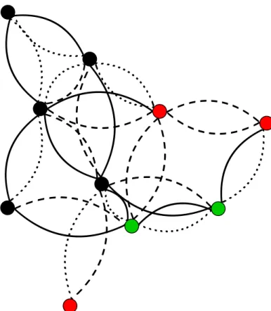
So far, we have basically presented random graph models aimed at modeling binary edges. In this section, we describe an extension of the SBM model, called the random subgraph model (RSM), as proposed by Jernite et al. (2014). The RSM model aims at modeling categorical edges using prior knowledge of a partition of the network into different subgraphs. Each subgraph is assumed to be
Figure 2.16: Example of an RSM network.
made of latent clusters which have to be inferred from the data in practice. Then, the vertices are connected with probabilities depending only on the subgraphs, whereas the edge type is assumed to be sampled conditionally on the latent groups.
An example of an RSM network is given in Figure 2.16. The node forms indicate the (known) partition of the network into S = 2 subgraphs. Moreover, the edge types Xij 2 {0, ..., C} (C = 3) are given by the edge colors. Within
each subgraph, the Q = 3 clusters are indicated by the node colors. As for the SBM and MMSBM models, the construction of the adjacency matrix is assumed to depend on latent clusters. Thus, each node i is first associated with an unobserved group among Q with a probability depending on si, where si
indicates the subgraph of vertex i:
Zi⇠ M(1, ↵si).
The vector ↵si denotes the cluster proportions for the corresponding subgraph.
Secondly, the presence of an edge between two nodes i and j is characterized by an observable variable Aij, such that Aij= 1is there exists a typed relation
between i and j, 0 otherwise. The edge type is then encoded by the observable variable Xij which takes its values in a finite set {0, 1, ...., C}.
The variable Aij is supposed to be drawn from a Bernoulli distribution
depending on the subgraphs si and sj only:
Aij ⇠ B( si,sj).
Then, if an edge is present between i and j, Xij is sampled from a multinomial
distribution with probabilities depending on the latent clusters. Xij|ZiqZjl= 1⇠ M(1, ⇧ql),
where ⇧ql2 [0, 1]C+1 andPCc=0⇧cql= 1.
Therefore, the model is defined through the following joint distribution: p(X, A, Z|↵, , ⇧) = p(X, A|Z, , ⇧)p(Z|↵)
= p(X|A, Z, ⇧)p(A| )p(Z|↵).
In the original paper, the inference is performed using a VBEM algorithm.
2.4 Clustering models for dynamic graphs
In Section 2.1, we defined some approaches capable of analyzing static networks. In this section, we now wish to extend models from the previous section to the dynamic framework. First, we introduce the dynamic mixed membership stochastic block model (dMMSBM), which is an extension of the static MMSBM model. Then, we present the dynamic SBM (dSBM) model, which extends the static SBM model.
2.4.1 Context and notations
We are now provided with a dynamic graph G where edges can appear or vanish over time. Conversely, the vertex set is assumed to be fixed. G is then defined through a series of T networks G = {G(t)
}T
t=1 where G(t) is a (fixed) graph at
time t. More precisely, G(t) is the (aggregated) graph of all the connections that
occurred during time frame t. In other words, in the binary case, two vertices iand j in G(t) are connected and the presence of the edge (i, j) is recorded if
there was at least one connection between i and j, during t. Furthermore, in the weighted case, the number of interactions for the edge (i, j) is recorded. As such, the dynamic network G can be seen as a time series of networks. Each graph G(t)is then represented by its N ⇥ N adjacency matrix X(t). Thus, in the
binary case X(t)
ij = 1if the edge (i, j) is present in the graph G(t), 0 otherwise.
Moreover X(t)
ij is set to the number of interactions that occurred during time
frame t, in the weighted case. Note that no self loops are considered here and therefore X(t)
ii = 0,8 i, t. In this context, clustering the data means clustering
the vertices at each time t.
2.4.2 Dynamic mixed membership stochastic block model
The dynamic mixed membership stochastic block model (dMMSBM) is a random graph model for dynamic binary graphs proposed by Xing et al. (2010). The idea at the core of this approach is to extend the MMSBM (Airoldi et al., 2008) model by including a state-space model to characterize the evolution of the latent space variables. Below, the model is presented in the case of directed graphs, where connections are oriented.
First, a vector (t)
i is considered for each node i at time t in the graph.