HAL Id: hal-00579839
https://hal.archives-ouvertes.fr/hal-00579839
Submitted on 25 Mar 2011
HAL is a multi-disciplinary open access
archive for the deposit and dissemination of
sci-entific research documents, whether they are
pub-lished or not. The documents may come from
teaching and research institutions in France or
abroad, or from public or private research centers.
L’archive ouverte pluridisciplinaire HAL, est
destinée au dépôt et à la diffusion de documents
scientifiques de niveau recherche, publiés ou non,
émanant des établissements d’enseignement et de
recherche français ou étrangers, des laboratoires
publics ou privés.
Volume-Aware Positioning in the Context of a Marine
Port Terminal
Yesid Jarma, Golnaz Karbaschi, Marcelo Dias de Amorim, Farid Benbadis,
Guillaume Chelius
To cite this version:
Yesid Jarma, Golnaz Karbaschi, Marcelo Dias de Amorim, Farid Benbadis, Guillaume Chelius.
Volume-Aware Positioning in the Context of a Marine Port Terminal. Computer Communications,
Elsevier, 2011, 34 (8), pp.962-972. �10.1016/j.comcom.2011.02.003�. �hal-00579839�
Volume-Aware Positioning in the Context of a Marine Port Terminal
✩ Yesid Jarma∗,a, Golnaz Karbaschib, Marcelo Dias de Amorima, Farid Benbadisc, Guillaume CheliusdaLIP6/CNRS – UPMC Sorbonne Universités, 4 place Jussieu, 75005 Paris, France bINRIA Saclay, Parc Orsay Université, 4 Rue Jacques Monod, 91893 Orsay Cedex, France
cThales Communications, 160 Boulevard de Valmy, 92704 Colombes Cedex, France dINRIA Rhône-Alpes, 655 avenue de l’Europe, Montbonnot, 38334 Saint Ismier Cedex, France
Abstract
The rapid proliferation of mobile computing devices and local wireless networks over the past few years has promoted a contin-uously growing interest in location-aware systems and applications. The main problem with existing positioning techniques is that they are designed to position dimensionless objects. Such an assumption may lead to practical inconsistencies, as it results in neglecting the effects of the volume of an object, its physical characteristics, and its spatial arrangement on signal propagation. In this paper, we consider the problem of positioning cargo containers in a marine port terminal, where such characteristics can be finely estimated. Based on the signal propagation map of a container yard, we propose VAPS, a volume-aware positioning system that takes advantage of the waveguide effect generated by the containers. Although VAPS is specific to the marine port scenario, its design principles can be extended and adapted to other situations. VAPS maps discrete RSSI levels into hop-counts and relies on realistic propagation models to obtain near-perfect positioning at a very low control overhead. Our extensive evaluations show how to set the parameters required in the VAPS algorithm. The results demonstrate that, in scenarios where the assumptions made by traditional approaches fail, the considerations of VAPS make the difference.
Key words: GPS-free positioning systems, signal propagation, waveguide effect.
1. Introduction
Having the coordinates of a node can be of great utility in numerous applications of wireless networks, including object tracking, warehouse inventory, health care, and environmental monitoring, to cite a few. Therefore, positioning systems have been and still are the focus of extensive research. The main approaches in use today rely on satellite-based systems such as GPS [1], Glonass [2], as well as the upcoming Galileo [3] and Beidou [4]. Although straightforward and widely adopted, satellite-based solutions cannot be used in a number of scenar-ios (e.g., indoor, underwater, and underground deployments) and can involve high economic and energetic costs. There have been many attempts in the literature to provide alternative solu-tions, commonly referred to as GPS-free positioning systems. These are roughly classified into two classes: signal-based and topology-based methods. In the first category, the strategy most frequently adopted is to measure the distance between the tar-get element and several reference points (whose coordinates are known) based on metrics such as the Received Signal Strength Indicator (RSSI) [5, 6, 7, 8, 9], Time of Arrival (ToA) [10],
✩This document is an extended version of our previous paper “VAPS: Posi-tioning With Spatial Constraints”, presented at IEEE WoWMoM 2009.
∗Corresponding author
Email addresses:yesid.jarma@lip6.fr (Yesid Jarma), golnaz.karbaschi@inria.fr (Golnaz Karbaschi), marcelo.amorim@lip6.fr (Marcelo Dias de Amorim), farid.benbadis@fr.thalesgroup.com (Farid Benbadis), guillaume.chelius@inria.fr (Guillaume Chelius)
Time Difference of Arrival (TDoA) [11], or Angle of Arrival (AoA) [12]. In the second category, the traditional approach is to determine the distance of a node to a number of refer-ence points by using network topology metrics such as the hop-count [13, 14, 15, 16]. In both methods, the coordinates of the target point are inferred through multi-lateration or similar techniques.
In this paper, we focus on a class of deployment scenarios where the abovementioned solutions cannot be used. In fact, existing methods are designed to position dimensionless nodes without considering their volume, physical composition, or any other spatial constraints. The implicit assumption is that the node to be positioned is a point in the space. This is a poten-tial source of errors because the volume, the physical charac-teristics of the objects to position, and their spatial arrangement may have a major impact on the signal propagation. The partic-ular characteristics of large objects may lead to new constraints such as a strong attenuation or reflection of propagated signals. In some cases, as the marine port scenario considered in this paper, objects have metallic surfaces that lead to high reflec-tion and blocking effects on the transmitted signals. Therefore, certain arrangements of metallic objects may cause waveguide effects, inducing homogeneous signal propagation throughout the area. Uniform propagation of signals may lead to ambiguity in determining the positions of the objects, as the signal atten-uation becomes completely different from the one observed in open spaces.
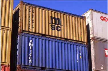
deal-Figure 1: Container yard in a marine port terminal.
ing with such specific challenges. In order to effectively bridge this gap, we propose VAPS, a Volume Aware Positioning Sys-temto position large metallic objects. Contrarily to traditional solutions, VAPS brings the following innovative features:
• Signal propagation-aware positioning. VAPS takes into account and benefits from the waveguide and blocking effects caused by metallic objects. This is fundamental in our scenario as these effects completely compromise the correlation between distance and reference parame-ters such as signal strength, propagation time, and angle of arrival. For this reason, in our scenario, traditional sys-tems are useless as they rely on such correlations when computing coordinates.
• Dimension-aware positioning. VAPS falls under the umbrella of hop-count-based systems; however, since con-tainers have well-defined dimensions, hop-counts can be directly translated into distances. Furthermore, VAPS is able to correct possible erroneous coordinates, therefore preventing physically impossible situations such as the overlap of two or more elements.
Taking spatial constraints into account is of course scenario-dependent. In this paper, we specifically refer to a reservoir of cargo containers at a marine port terminal arranged along long rows, several containers high, in a limited space. The contain-ers are metallic, inducing high reflection, which leads to dis-tinct waveguide effects. This means that signal attenuation in the space separating two rows of containers is almost null. By applying realistic signal propagation that we obtained through extensive simulations, we show that: (i) VAPS works where traditional solutions are unfeasible (ii) VAPS leads to highly accurate positioning, and (iii) VAPS is energy-efficient by gen-erating very low control overhead.
The remainder of this paper is structured as follows. In Sec-tion 2, we describe the context of the paper, and in SecSec-tion 3 we illustrate the particularities of signal propagation in position-ing metallic objects with large dimensions. In the same sec-tion, we clearly state the problem of using traditional methods
Figure 2: Stacks of cargo containers in a marine port terminal.
when attempting to position metallic objects with large dimen-sions. Section 4 presents the VAPS algorithm for positioning cargo containers, while Section 5 evaluates our algorithm via simulations. In Section 6 we discuss the performance of our al-gorithm and give insights on remaining open issues. Section 7 gives an overview on prior works in positioning algorithms for multi-hop wireless networks. Finally, we conclude the paper in Section 8.
2. Context
During the latest decade, the world has been shaped by the influence of globalization. To sustain economic growth, many companies have started to develop new markets outside their home countries. Therefore, international transportation systems became under increasing pressures to support additional de-mands. The introduction of cargo containers resulted in consid-erable improvements in efficiency, lowering costs, and boosting global trade flows.
The target scenario considered in this work is the localiza-tion of cargo containers in a marine port terminal.1 Many mod-ern marine ports are used as intermediate destinations where the cargo is changed form one transportation method to another. In large ports, such as the one depicted in Fig. 1, cargo container facilities may extend over 170 hectares, where several thousand containers are held and moved every day. Clearly, locating and tracking such a large number of containers require complex lo-gistics.
When cargo containers are being held in the port, they are usually stacked one on top of another, with little vertical space between them (about 10 cm), and narrow aisles (about 1 m) separating two rows of stacks (see Fig. 2). A row of stacks may be up to 100 meters long, and 20 meters high. This particular arrangement and the metallic composition of cargo containers both have an impact on the propagation of signals between two
1More specifically, this scenario is the one addressed in the context of the French project “Watch and Warn” in collaboration with the Le Havre har-bor [17].
(a) Above view. (b) Transversal view.
Figure 3: Signal propagation of a sensor in a field of rectangular metallic objects (dark rectangles represent containers). A white “X” represents the transmitting sensor. 0 5 10 15 20 25 30 35 0 20 40 60 80 100 120 Attenuation (dBm) Distance (meters)
(a) Attenuation in an aisle between two stacks of containers.
0 20 40 60 80 100 0 1 2 3 4 Attenuation (dBm)
Aisles away from transmitter
(b) Attenuation from one aisle to another. Figure 4: Observed Path Loss Model. Vertical error bars represent the tolerance.
rows of stacks of containers. These particularities are described and analyzed in the following section.
3. Problem Statement
3.1. Analyzing the waveguide effect
To better assess the effects of the particular arrangement and characteristics of these objects on wave propagation, we con-ducted a set of precise radio propagation simulations. To this end, the WILDE (WIreless LAN DEsign) tool was used [18, 19]. Fig. 3 illustrates the obtained results. In these figures, dark rectangles represent the containers disposed in rows; one wire-less sensor (placed on the longest surface of a container and represented with the white ‘X’ in both figures) sends a signal whose RSSI is measured in the rest of the space. The RSSI is represented by colors. In the aisles where the signal is transmit-ted, the color is something between red and orange, meaning that the signals are received with almost the same power-level they were transmitted. In the following aisles, where the colors are yellow, green, or blue, the received signals are attenuated. This attenuation, however, happens sharply, and the power level
remains almost constant all along the same aisle (except for the border effect at crossing points).
In these results, two particular phenomena can be observed. First, wave propagation in the aisles between two rows of stacks of containers closely resembles a waveguide. Nevertheless, it is not a tuned waveguide and therefore path loss occurs. Fig. 4(a) shows the observed path loss model for an aisle between two rows of stacks of containers. Error bars represent an error mar-gin of ± 5dBm. Since the attenuation inside an aisle is well below the sensitivity threshold, any node transmitting inside an aisle can be heard several hundred meters away. Clearly, the observed model greatly differs from the traditional free-space path loss model, where the typical range is around 50 meters.
The second observed phenomenon is that the objects act as barriers. The metallic nature of cargo containers and their size prevent the signals from reaching near points. This behavior is illustrated in Fig. 4(b). Error bars represent an error margin of ± 15dBm. Even if two adjacent aisles between containers are a few meters away from each other, the attenuation changes abruptly from one aisle to the next. Nevertheless, all along one aisle, wave propagation continues to follow the waveguide-like
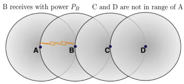
A B C D
B receives with power PB
B distance estimate is d(PB)
C and D are not in range of A
C and D can’t estimate distance to A
(a) In open space, node B is in range of node A and can estimate its distance to it. Nodes C and D are outside node A’s range.
A B C D
B, C and D receive with powers PB≈ PC≈ PD
B, C and D distance estimates are d(PB) ≈ d(PC) ≈ d(PD) (b) Inside a waveguide, nodes B, C and D are in range of node A and can estimate its distance to it. However, because of homogeneous signal propagation they will estimate they are closer than they actually are. Figure 5: Distance estimation using RSSI in open space and inside a waveguide.
A B C D
(a) In open space, node A communicates with nodes C and D in a hop-by-hop way.
A B C D
(b) Inside a waveguide, node A can communicate directly with nodes C and D.
Figure 6: Distance estimation counting number of hops in open space and inside a waveguide.
path loss model observed in Fig. 4(a). Therefore, the attenua-tion is almost homogeneous along an aisle.
3.2. Limitations of existing approaches
To our knowledge, all existing positioning methods assume that objects are just small points in space, without any dimen-sions whatsoever. Moreover, there is no consideration of the effects that the volume and physical characteristics of an object may have on signal propagation. Therefore, given the particular characteristics of wave propagation in the previously presented context, any attempt to position large metallic objects using ex-isting techniques will lead to considerable positioning errors. To better illustrate this, we analyze the issues that rise when two of the most popular positioning techniques are used to po-sition objects inside a waveguide. Further details on existing techniques are presented in Section 7.
One of the most used techniques consists in estimating the distance between an object and at least three reference points whose positions are known. Then, by trilateration, the object calculates its position relatively to the positions of the reference points. The distance between two nodes can be calculated us-ing for example the RSSI. If both nodes are identical (i.e., they transmit with the same power and they have the same sensitiv-ity threshold) the receiving node can estimate its distance to the transmitting node by using the RSSI and a path loss model. In Fig. 5(a), we represent a topology with four nodes. Here, node B is the unique node under the coverage range of node A, and therefore it can accurately estimate its distance to node A by using RSSI and a free-space path loss model [20]. Since nodes
C and D are outside A’s range, they cannot estimate their dis-tance. In contrast to a free-space model, inside a waveguide (see Fig. 5(b)), nodes B, C, and D are all in the communica-tion range of node A, and can thus estimate their distance to it. However, because of the particularities of signal propagation inside a waveguide, all four nodes will receive the transmitted signal with almost the same power. By using a free-space path loss model, they will estimate their positions to be closer than they actually are.
Another technique consists in measuring the distance from a node to a reference point in number of hops. This information can be then used to calculate a distance in meters, or directly as coordinates. In Fig. 6(a), nodes A, B, C, and D communicate with each other in a hop-by-hop fashion. In this case, node D is three hops away from node A. Inside a waveguide, node A can communicate directly with nodes B, C, and D. In such a case, the use of a hop-count technique attributes the same coordinates to those three nodes, although they are placed at significantly different distances from node A.
4. VAPS: Volume-Aware Positioning System
To address the new challenges in positioning with spatial constraints, we adopt a strategy that differs from those of tra-ditional approaches. We mainly undertake two actions. First, every object should be equipped with more than one communi-cating device (or sensor) so that we can integrate the notion of dimension. We assume that the sensors on the same object are wired to each other and exchange positioning information
be-Figure 7: This figure shows a grid of 16 objects with three sensors each to enable three dimensional positioning. The sensors are represented by blue cir-cles, and are wired to each others. Note that all sensors are facing the same directions.
tween them instantly, and without consuming any wireless re-source. In the description of the algorithm, we call these nodes corresponding nodes. Fig. 7 shows an example of node equip-ment for three dimensional positioning. In this particular ex-ample, each object is equipped with three nodes (one for each dimension) wired to each others. Note that all nodes are on the exact same surface on each object and therefore they all have the same direction. Second, we consider in the design of our algorithm the effects that metallic objects may have on signal propagation, namely the waveguide effect. In this section, we first specify the preliminaries of our approach. The details of VAPS come thereafter.
4.1. Determining N discrete distinguishable power levels Without loss of generality, we assume that all sensor nodes have the same transmission power Pr and the same sensitiv-ity threshold. As a consequence of the waveguide effect, sig-nal propagation in an aisle is almost homogeneous; therefore a transmitting node is heard with almost the same reception power all along the aisle it is placed in. Using this particular phenomenon, we can easily conclude that every node hearing the maximum received power level are estimated to be in the same aisle as the transmitting node. The transmitted signal will propagate throughout the area and it will be heard in the ad-jacent aisles, but with an attenuated power level. As observed in Fig. 3, the attenuation happens sharply. This attenuation, however, follows the waveguide effect and thus remains almost constant all along the same aisle.
We assume that, in general, a transmission originated inside any aisle can be heard at the next N consecutive aisles. Using the particular waveguide/blocking effects of this context, we are able to define N discrete and clearly distinguishable power lev-els. The number of power levels is determined by the number of aisles away from the transmitting node where the RSSI is
X 80 - 75 % 50 - 45 % 25 - 20 % 5 - 0 % 5 - 0 %
Figure 8: This figure shows a situation where X’s signal is easily distinguish-able from an aisle to another till the third aisle. The received signal at the forth and fifth aisle is just below the sensitivity threshold of the sensors.
above the sensitivity threshold of the nodes. To better illustrate this, we take as example the topology depicted in Fig. 8.
In this particular case, there are 25 rectangular metallic ob-jects arranged in a 5 × 5 grid. We set a transmitting node, rep-resented with a white “X”, in the lower side of the container located at the top left corner of the topology. Other nodes (not depicted in the figure) located in the lower sides of the rest of the containers measure the power of the received signal. In this example, we assume that the sensitivity threshold is 20% of the original power. When the transmitting node sends a message, the nodes located on the same aisle as the transmitter receive the signal with 80 – 75 % of its transmitting power. Nodes lo-cated one aisle away will receive the signal with 50 – 45 % of its original power, while nodes two aisles away will receive the signal with 25 – 20 % of its original power. For the nodes lo-cated three and four aisles away, the received signal will be just below their sensitivity threshold. Nodes in the first three aisles can easily detect the signal, and the receiving power from one aisle to the next one is clearly distinguishable. On the other hand, there is no clear distinction between the power received in the fourth and fifth aisles, and in some cases, a number of nodes will not be able to detect the transmission. In this partic-ular example, N is thus set to 3. It means that one transmission in an aisle is able to determine the aisle number of objects of three aisles.
The value of N depends on several factors, including the reception sensibility of the sensors, the width of the aisles, pos-sible changes in the propagation characteristics of the wireless medium, and the transmission power Pr. Note that the value of N can be different across each direction. In the example de-picted in Fig. 8, horizontal aisles are wider than vertical aisles, and consequently the waveguide effect in the former is more important than in the latter. Therefore, in the general case, we consider Nxand Nyas different values for each direction. 4.2. Description of the algorithm
For the sake of presentation, we consider a two-dimensional space with two axes X and Y. Nevertheless, extending the
al-gorithm to three dimensions is straightforward.2 Let L ibe the power level measured at aisle i from the emitter and V = {L1, . . . ,LN} be the set of these measurements (i = 1 means the same aisle of the emitter). An object (i.e., a container) has two sensors placed on orthogonal surfaces. We refer to these sensors as corresponding nodesand call them x-node and y-node respec-tively to the axis they contribute to. The objects are assumed to have a direction, such that x-nodes and y-nodes are placed on the same surface on each one of the containers. We compute coordinates with regard to an object placed in a corner of the topology whose coordinates are, by definition, (X = 0, Y = 0). We refer to this particular container as the anchor. Note that we need only one anchor.
The anchor starts the positioning process by broadcasting a message toward the x-axis (via its x-node). To prevent possible collisions that may interfere with positioning, we introduce a back-off time when broadcasting toward the axis (via its y-node). Messages broadcasted toward the x-axis determine the column number and toward the y-axis the row number. Each message contains two pieces of information: a coordinate (X or Y), and the axis it corresponds to. A node that receives a message analyzes the axis information to determine whether it should process the message or not: x-nodes only process x-axis messages while y-nodes only process y-axis messages. If the message is processed, the positioning information together with RSSI information is analyzed. If the message is received with a RSSI that is within the range [L1; L2[, then the receiving node assumes it is located in the same row/column as the sender and sets its corresponding coordinate as the same as the sender’s one. Similarly, if the message is received with an RSSI within the range [L2; L3[, the receiving node is located one row/column away from the sender and it sets its corresponding coordinate to Xsender+1 (or Ysender+1). Note that intervals must be left-closed to avoid misinterpretation of the row/column to assign to a node. This procedure is performed by all nodes up to the (Nx− 1)thcolumn (resp. (N
y−1)throw). In all cases, a receiving node notifies the new coordinate to the second corresponding node on the same object. The procedure is summarized in Algorithm 1. 4.3. Reducing the number of broadcasted messages
One of the issues in most of the positioning algorithms is the large amount of messages exchanged between nodes. The consequences are, in general, higher energetic costs, collisions, and an overall decrease in protocol performance. In order to limit the number of messages used for positioning, and to pre-vent collisions, some actions are undertaken. First, since we assume that a broadcasted message can be heard as far as the (Nx−1)thcolumn (resp. (Ny−1)throw) away, we set the restric-tion that only the nodes that are in the (Nx−1)thcolumn (resp. (Ny−1)throw) rebroadcast the positioning messages. The total number of broadcasted messages, called T , is computed as:
T = R & C (Nx−1) ' + C & R (Ny−1) ' ,Nx,Ny>1 (1)
2Since the signal propagation model in the ZY plane is similar to the one observed in the XY plane, it suffices to apply, in addition, the same algorithm in this new plan (ZY) to get a three dimension positioning.
Algorithm 1 VAPS algorithm
VX= {L1,L2,L3, ...,LNX−1,LNX}
VY= {L1,L2,L3, ...,LNY−1,LNY}
Positioning message = (COORD, AX), AX = {X, Y} if AX = My axis then
if RSSI > LNAXthen
for i = 0 to i < NAXdo
if RSSI ≤ VAX[i] and RSSI > VAX[i + 1] then if COORD < My Coordinate then
My Coordinate = COORD + i
Send My Coordinate to Corresponding Node end if
end if end for
else if RSSI ≤ LNAXand RSSI > S ensitivity then if COORD < My Coordinate then
My Coordinate = COORD +(NAX−1) Send My Coordinate to Corresponding Node Broadcast My Coordinate
end if end if else
drop the message end if
where C is the number of columns and R is the number of rows. Thus, the number of positioning messages broadcasted is re-duced when compared to other traditional approaches where all nodes rebroadcast the positioning messages.
Second, besides triggering different start times for the posi-tioning algorithm at each axis, VAPS includes a back-off pro-cedure for rebroadcasting the positioning message reaching the (Nx−1)thcolumn (resp. (Ny−1)th). This procedure is similar to the collision avoidance procedure used in channel access algo-rithms. Upon reception of a positioning message, nodes in the (Nx−1)th column (resp. (Ny−1)th row) set up a timer with a random delay to retransmit the positioning message. The node whose timer expires first rebroadcasts the positioning message. The other nodes in the same row/column overhear this trans-mission and cancel their own transtrans-mission. More specifically, before canceling their transmission, these nodes first verify if the reception has been performed at the highest power and if the coordinate is the same as the one they have already stored.
It is worth mentioning that there is a tradeoff between the number of broadcasted messages and the accuracy and robust-ness of the system. Consider an ideal scenario where the area conditions allow the definition of N ≥ max(C, R) distinguish-able power levels. In such an ideal case, one positioning mes-sage per axis would be enough in order for every objects in the network to estimate its column and row number. Nevertheless, in this case, even mild changes in the propagation conditions may trigger positioning errors.
4.4. Measuring the real distance between the nodes
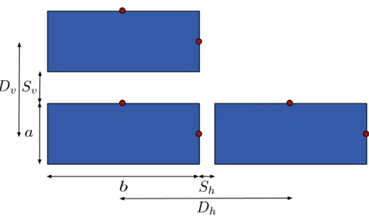
Since the dimensions of the objects and their arrangement are known beforehand, it is possible to easily and precisely cal-culate the distance between objects by using hop-count infor-mation. Let the objects be rectangular with height a and length b. They are arranged on a grid with a vertical space Sv and horizontal space Sh between them as depicted in Fig. 9. The
Dh DvSv
Sh a
b
Figure 9: Calculation of the distance between containers.
vertical distance Dv(resp. horizontal distance Dh) between the center of an object and the center of the next object is calculated as Dv =(a + Sv) (resp. Dh =(b + Sh)). Therefore, the verti-cal (resp. horizontal) distance between an object, and another located n hops away is Dv= n(a + Sv) (resp. Dh= n(b + Sh)). 5. Evaluation
To study the performance of VAPS, we evaluate it in a sim-ulation environment adapted to our needs. Castalia [21, 22] is a Wireless Sensor Network (WSN) simulator based on the OMNeT++ Discrete Event Simulation System [23]. Castalia mainly focuses on providing a realistic wireless channel and ra-dio model, with a realistic node behavior especially relating to access of the radio. The algorithms are written in C++ and they are event driven, where an event can be an incoming message or a periodic timer. The OMNeT++ library controls the sim-ulated time and the concurrent execution of the code running at each node. In the remainder of this section, we first discuss some specific implementation details of our simulations before presenting the results.
5.1. Simulation settings
In order to perform a set of simulations that closely rep-resent real-life conditions, the interference model used in our simulations is assumed to be an additive model, in which all the transmissions heard by a receiver are added to the background noise as the interference level of the area. To accommodate the simulations to the particular propagation characteristics of the target scenario, we introduce the waveguide effect by setting signal propagation along an aisle between two rows of contain-ers in an almost homogeneous way, with very low power atten-uation. Note that this has a direct impact on communications, as it causes transmissions to be more prone to collide with each other.
One of the features of Castalia, besides providing a wireless channel propagation model, is that it allows the manual defini-tion of connectivity between pairs of nodes, by specifying the received power level in dBm at one node, when the transmis-sions come from another node anywhere in the topology. We
used this unique feature in order to manually define the partic-ular connectivity between nodes according to the propagation characteristics of the scenario under consideration. Accord-ing to the characterization we performed with WILDE, in the considered scenario there are three clearly distinguishable dis-crete power levels (N = 3); we set these to L1=0dBm, L2 =-30dBm, and L3=-60dBm. Nevertheless, a manual definition of the reception level at one node would imply that all the received messages from another node arrive with the exact same power level each time. To introduce randomness in this process, and therefore obtain more realistic results, we add a random value extracted from a Gaussian distribution with zero mean and a pa-rameterized standard deviation σ to each reception power level. Several simulation runs were conducted to evaluate the po-sitioning error of VAPS. All data points shown on the curves represent an average over 50 runs within 95% confidence in-terval. The simulated topology contains 100 containers mea-suring 10 × 4 meters. This results in a total of 200 nodes, as each object is equipped with two sensors wired together (recall that we perform simulation only for the two dimensional case). We assume that all nodes have the same reception sensitivity (-95dBm) and identical maximum transmission power (10 dBm). Furthermore, as we focus on the positioning error, we assume that no packet loss occurs, however by using the back-off pro-cedure in VAPS packet loss may occur rarely. The average po-sitioning error is computed with the following equation, which is widely used in previous works:
Erravg= PM i=1 q (xi−x′i)2+(yi−y′i)2 M , (2)
where M is the number of nodes, (xi,yi) is the real position of node i and (x′i,y′i) is the estimated position of node i.
As in a real marine port terminal, containers are placed fol-lowing a grid pattern on a 122 × 62-meter field. The anchor object is placed at the bottom left corner of the field. All ob-jects are 1-meter apart horizontally and 2-meters apart verti-cally. Consequently, the waveguide effect is more accentuated in the horizontal aisles than in the vertical aisles.
5.2. Analysis of the retransmission at the Nthlevel
Since we assume that a broadcasted message can be heard as far as the Nthrow/column away, in our algorithm we set the restriction that only the nodes that are in the Nth row/column rebroadcast the positioning messages. As one of the motiva-tions for this choice is to reduce positioning errors induced by collisions, we evaluated the impact of this choice on the perfor-mance of the algorithm. We consider three different values of N = {1, 2, 3}.
Fig. 10 illustrates the average positioning error for retrans-mission at different aisles. Under ideal propagation conditions (σ = 0), when retransmitting at every aisle (N = 1), every two aisles (N = 2), and every three aisles (N = 3), the average positioning error is zero hop. In the presence of mild changes on propagation conditions (σ = 6), retransmitting at every aisle leads to higher positioning errors (about 0.4 hops), than retrans-mitting every two and every three aisles (close to zero). When
0 0.5 1 1.5 2 2.5 3 0 2 4 6 8 10 12
Avg. Positioning Error (hops)
Std. dev (σ) N = 3
N = 2 N = 1
Figure 10: Average positioning error vs. Standard Deviation σ for message retransmission at different aisles.
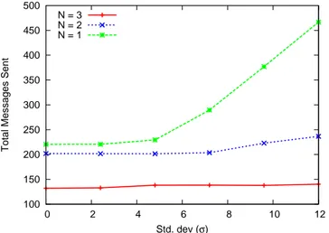
100 150 200 250 300 350 400 450 500 0 2 4 6 8 10 12
Total Messages Sent
Std. dev (σ) N = 3
N = 2 N = 1
Figure 11: Total number of sent messages for message retransmission at differ-ent aisles.
there are considerable changes (σ = 12) on propagation con-ditions, when retransmitting at N = 1 the average positioning error is 2.8 hops, at N = 2 is 1.4 hops, and at N = 3 is 0.8 hops. Clearly, by restricting the retransmissions to occur only at the last distinguishable level, the algorithm obtains a superior performance, since the possibility of collisions is reduced.
Another motivation behind the choice of retransmission at the Nth row/column is to reduce the number of messages used for positioning proportionally to 1/N. This is what we observe in Fig. 11, which shows the total number of messages trans-mitted for each setting. When retransmission is done at each reception (N = 1), the total number of transmitted messages can reach 460 in the presence of considerable changes of prop-agation conditions. Retransmitting every two aisles results on a clear drop in the total number of messages to around 240. By setting the retransmissions at N = 3, the total number of re-transmissions is reduced to 140. Reducing the total number of messages has a direct impact on the protocol costs in terms of control message overhead and energy.
0 50 100 150 200 0 2 4 6 8 10 12
Total Messages Sent
Std. dev (σ)
Backoff = 0 ms Backoff = 30 ms Backoff = 50 ms Backoff = 55 ms
Figure 12: Total number of sent messages for different Back-off values.
0 0.2 0.4 0.6 0.8 1 0 2 4 6 8 10 12
Avg. Positioning Error (hops)
Std. dev (σ) Backoff = 0 ms
Backoff = 30 ms Backoff = 50 ms Backoff = 55 ms
Figure 13: Average positioning error vs. Standard Deviation σ for different Back-off values.
5.3. Impact of the back-off procedure
As previously stated, we also introduce a back-off proce-dure to to further improve the performance of the algorithm and to reduce the number of messages used for positioning. The idea is to take advantage of the waveguide effect present in the aisles between containers.
To choose an appropriate value for the back-off timer, we conducted a set of simulations. Fig. 12 shows the total number of transmitted messages as a function of the standard deviation σ. The duration of the back-off timer is varied from 0 to 55 ms. As shown in this figure, without the back-off procedure, the total number of messages sent is about 130. This number is reduced down to 25 by increasing the back-off timer. When there are changes in the propagation conditions, the number of used messages increases. This is mainly due to nodes not being able to hear the transmission of the node whose timer expires first, and therefore triggering their own transmissions at the end of their timer.
Fig. 13 compares the average positioning error for different values of the back-off timer. In the figure, under ideal
0 1 2 3 4 5 6 7 8 0 2 4 6 8 10 12
Avg. Positioning Error (hops)
Std. dev (σ) VAPS
VCap APS
Figure 14: Average positioning error vs. standard deviation σ for different approaches.
tions (σ = 0) the positioning error is zero for all back-off val-ues except for 55 ms, where it is around 0.3 hops. With strong variations in the RSSI (σ = 12), the average positioning error is about 0.7 hops when there is no back-off procedure, 0.8 for 30 ms and 50 ms, and around 0.7 for 55 ms. We can notice the fact that setting the back-off timer to a very large value (e.g., 55 ms) induces errors even with mild variations in the propaga-tion condipropaga-tions. It suggests that there is a trade-off between the duration of the back-off timer and the accuracy of the system. The trade-off occurs because with large back-off timer values, the number of retransmitted messages is greatly reduced. This may lead to some cases where one or several nodes are not able to obtain their correct coordinates and thus the average position-ing error of the system is increased. Since our system considers the volume and the spatial arrangement of the objects, when the average positioning error is below 0.5 hops (represented by a horizontal dotted line), it can be approximated to zero. There-fore, setting the back-off timer to 50 ms is a good candidate for the rest of the simulations.
5.4. Comparison with other approaches
We compare the performance of VAPS with two other algo-rithms (signal and topology based). The first algorithm, APS [6], uses only the RSSI and a free-space path loss model to esti-mate the distance from an object to a number of landmarks with known coordinates, and then trilateration to calculate the coor-dinates. A total of nine landmarks that broadcast periodic bea-cons are used to cover the whole area. The second algorithm is vCap [14], where the objects estimate their hop-count dis-tances to three landmarks, and use this information directly as coordinates. Both APS and vCAP are explained in Section 7.
We first investigate the advantages of VAPS without ap-plying the back-off procedure. The idea is to show that, even without using the back-off timer, VAPS outperforms the other approaches. Fig. 14 shows the average positioning error as a function of the standard deviation σ. The results show that, un-der ideal conditions (σ = 0), the positioning error is about 6
0 1000 2000 3000 4000 5000 6000 0 2 4 6 8 10 12
Total Messages Sent
Std. dev (σ) VAPS Backoff = 50 ms
VAPS No Backoff VCap
Figure 15: Total number of sent messages for different approaches.
0 2 4 6 8 10 12 0 2 4 6 8 10 12 14 16 18
Avg. Positioning Error (hops)
Manhattan Distance (hops) VAPS (σ) = 2.4
VAPS (σ) = 12 VCap (σ) = 2.4 VCap (σ) = 12
Figure 16: Average positioning error vs. Manhattan Distance for different ap-proaches.
hops for the RSSI-based method, 5 hops for vCap, and 0 for VAPS. When there are strong variations in the RSSI at each node (σ = 12), the RSSI-based method and vCap obtain the same values as before, while VAPS achieves an average posi-tioning error of 0.8 hops.
The comparison is further investigated in Fig. 15, which shows the total number of messages generated by vCap and VAPS. The results for APS are not shown since the number of messages generated by this algorithm is equal to the number of landmarks multiplied by the number of beacons they have sent during the simulation – i.e., there are no message retransmis-sions at the nodes. For vCap, the total number of transmitted messages is about 4,000 under ideal conditions, and increases up to 5,000 in the presence of considerable variations in the propagation conditions. VAPS dramatically reduces this num-ber to around 130 (σ = 0) and to around 140 for σ = 12 without the use of a back-off procedure. By using a back-off of 50 ms, this value is further reduced to 25 under ideal conditions, and around 40 when the propagation conditions are highly variable. This reduction has a direct consequence on the protocol cost in
0 0.5 1 1.5 2 2.5 3 0 2 4 6 8 10 12
Avg. Positioning Error (hops)
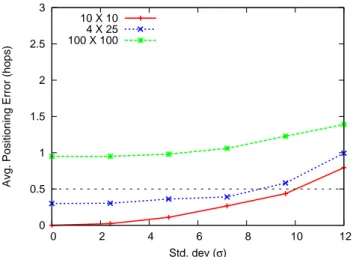
Std. dev (σ) 10 X 10
4 X 25 100 X 100
Figure 17: Average positioning error vs. standard deviation σ for different topology sizes.
terms of control message overhead and energy.
To show how the positioning error is propagated away from the anchor object, we measure the average positioning error as a function of the Manhattan distance [24]. Again, the results for APS are not shown since, with this algorithm, the coordinates are calculated by each node with the information they receive from the landmarks, and therefore coordinate information is not propagated away from each landmark in a hop-by-hop fashion. Fig. 16 shows the results. We consider only the simulations where the standard deviation is 4 and 12, since these two val-ues simulate respectively mild and considerable changes in the propagation conditions. In both cases, when the objects are rel-atively close to the anchor node (3 hops away), the average po-sitioning error is around 1 hop for the hop-count-based method, and below 0.5 hops for VAPS. For VAPS, these errors can be approximated to zero, since it considers the volume and spatial constraints for the objects. For objects that are more than 14 hops away from the anchor node, the average positioning er-ror for these standard deviations is about 8 hops for vCAP (for both τ = 4 and τ = 12), while it is 0 hops and 1 hop for VAPS, respectively. This figure shows that the capacity of VAPS to correct some degrees of positioning error lead to very low er-rors even in positioning far objects.
5.5. Impact of the Size of the System
In Fig. 17, we explore the performance of the algorithm in larger topologies. We chose two different sizes: 4×25 which contains the same number of nodes, but is larger towards the x-axis, and 100×100 which contains 100 times more nodes. We deliberately chose not to include any modifications to the al-gorithm, such as changing the location of the anchor node or adding additional ones. As expected, for larger topologies, the performance of the algorithm is slightly degraded. Since the aisles are longer on the x-axis, the nodes that are the farther away from a transmitting node will receive a more attenuated signal, which may cause a node to be unable to distinguish the row it is on, thus inducing positioning errors.
6. Discussion
Feasibility. It is clear that there is a class of deployment scenar-ios where signal propagation does not follow the traditional free space [20] or indoor [25, 26] propagation models. In these par-ticular cases, the use of existing positioning methods (cf. Sec-tion 7) may lead to considerable posiSec-tioning errors. The results shown in Section 5 highlight this fact. Consequently, existing positioning methods are simply unfeasible in such a deploy-ment scenario. VAPS was designed to provide accurate posi-tioning in cases where the spatial arrangement and the physical composition of the objects have a major impact on signal prop-agation. Along these lines, our algorithm proved to be superior to existing approaches.
Efficiency. In the scenario tackled in this paper, the choice of the number of levels, as well as their values, aimed at reduc-ing the impact of changes in propagation condition changes on the accuracy of the algorithm. VAPS also relies on a back-off procedure and on limited retransmissions to reduce the number of messages used for positioning. Although this increases the probability of missing a message, the reduction in the number of positioning messages leads to significant improvement of the system’s efficiency. The reduction of interfering collisions fa-cilitates the computation of exact coordinates, while reducing the signaling cost of the algorithm. Indeed, since our algorithm is able to use less signaling traffic, it is less penalizing to con-current applications.
Energy Consumption. VAPS was designed to work with wire-less communication protocols adapted to embedded applica-tions requiring low power consumption, such as IEEE 802.15.4. Moreover, by using fewer messages, there is a lower consump-tion of energy. As one of the main concerns when deploying wireless applications is the autonomy of the system, a prelimi-nary task such as positioning should not consume the energetic resources of the nodes. VAPS reduces the energetic cost of the system, therefore allowing other applications to run longer. Environment knowledge. One of the distinct features of our algorithm is its ability to map a number of clearly distinguish-able discrete power levels into hop-counts. In order to accu-rately define the number of power levels to be used, and the range of values every level should represent, the propagation conditions must be studied and analyzed prior to launching the algorithm. Additionally, since our approach is addressed to a class of scenarios where wave propagation follows particular characteristics, it is clear that this study must be conducted for each scenario and will most likely lead to a different set of power levels each time. The careful definition of the number of power levels to use and their values are fundamental for the good operation of our approach. Also, as the dimensions of the objects and their specific arrangement are known beforehand, VAPS has the ability to correct positioning errors when they are below 0.5 hops. The conducted simulations showed that, even if the approach is sensible to changes in the propagation condi-tions, only considerable changes induce errors in the algorithm, and those errors are nonetheless under 1 hop.
Open issues. Even though our approach was conceived to pro-vide accurate positioning in real life deployment scenarios with particular wave propagation, it has been so far evaluated through simulations. Although these simulations were conducted using tools that closely reproduce the conditions found in a real life scenario, it is not possible to take into consideration all the fac-tors that could affect the performance of the algorithm. Conse-quently, real wave propagation data obtained at a marine port terminal is needed to complement the data obtained from simu-lations. Additionally, a real life deployment is needed in order to evaluate the performance of the system and to introduce fur-ther improvements.
The results shown in Section 5 illustrate that VAPS cannot scale to infinity. It is expected, as waveguide are not perfect, and dispersion is expected. Nevertheless, even in larger topolo-gies the performance of VAPS is superior to the performance of existing positioning algorithms. A future version of the al-gorithm should include the necessary adjustments (e.g., addi-tional anchor nodes and addiaddi-tional retransmissions) in order to deal with the issues.
In this paper, we did not consider the case where one or more objects are missing, In this case, when the topology in-cludes “holes”, the propagation conditions would most certainly change in some areas, and would probably lead to inaccurate positioning. A future version of the algorithm should include a contention mechanism, where the system is able to detect one or several objects missing, and act accordingly in order to re-duce the effects this particular situation might have on the per-formance of the algorithm.
VAPS does not consider cases where objects are able to move around and change positions. In these cases, positioning error will be induced by objects moving out of the coordinate where they were located initially, and propagating wrong coor-dinates to adjacent nodes. We also plan to include such a feature in a future version of the algorithm, by determining how often the algorithm should be re-run.
Our algorithm was conceived to position objects with a vol-ume, and as such, in its design we take into account the three-dimensional case. However, in order to simplify the analyses, and due to the limitations of the tools used for evaluating our approach, the description of the algorithm, as well as its eval-uation, only include the two-dimensional case. Nonetheless, the extension of the algorithm to the three dimensional case is straightforward.
7. Related work
Ever since the appearance of the Global Positioning System (GPS) and the multi-billion dollar market it spawned, the po-sitioning of objects has been a widely studied research subject. The existing positioning methods can be divided into two cat-egories: signal-based methods, where the distance between a point and several reference points with known positions is esti-mated or calculated and then, by trilateration or other methods, the position of the point can be determined; and topology-based methods, where a node position is determined by using network topology metrics such as the hop-count between nodes.
Most of the current positioning techniques are based on physical measurements of signal propagation. Some methods use the RSSI in order to estimate the distance between a node and a reference point. RSSI is a measurement of the power of a received radio signal. Using this measurement and a propaga-tion loss model, distance from a point in space to a radio source can be easily estimated. The RADAR Location System [5] uses RSSI information in order to locate and track a node in-side a building. This system relies on an off-line data collection phase, where three base stations will record RSSI information from nodes in order to construct a map of the area. After this phase, a node is able to infer its position by comparing its RSSI measurements with the previously recorded data. Niculescu et al. propose Ad hoc Positioning System (APS) [6], which is a simplified version of GPS. To calculate its position, a node es-timates its distance to a minimum of three landmarks by using RSSI or by using a distance vector algorithm if the node is mul-tiple hops away from the landmark. Hop-TERRAIN [7] uses a similar approach to estimate the position of a node, which will then be iteratively refined to improve accuracy. Niculescu et al. propose in [29] a comprehensive survey on these techniques.
More recently, several research efforts have been oriented towards the use of topology metrics in order to determine the position of a node. GPS-Less [30] needs a limited number of nodes with known positions and overlapping regions of cover-age to serve as reference points that periodically transmit bea-con signals bea-containing their position. Each node will infer its proximity to a set of reference points when the ratio of received to sent beacons metric surpasses a certain threshold. A node locates itself to the region where the coverage regions of these reference points intersect. In No-GEO [13], Rao et al. pro-pose a system where the nodes are able to find their positions from the edge of the network towards the center of the network. Two designated bootstrap nodes broadcast beacons to the en-tire network. Nodes use their hop-count distances to one of the bootstrap nodes to determine whether they are perimeter nodes. Then every perimeter node broadcasts a message to the entire network, allowing other nodes to compute a vector containing their distance to all perimeter nodes. Using inter-perimeter dis-tances, each node calculates normalized coordinates for both itself and the perimeter nodes by running a relaxation algo-rithm. With each iteration, a node will compute its position based in the position of its neighbors. The resulting position of a node is the average of its neighbors’. Caruso et al. propose vCap [14], a three-dimensional coordinate system based only in the hop-count distances between nodes. After network deploy-ment, three nodes located on the edge of the network will be se-lected as anchors. These anchors will broadcast, one at a time, an election message to the entire network so that each node can calculate its own hop-count distance to each anchor. These dis-tances will be directly used as three-dimensional coordinates. A similar approach, called GPS-Free-Free, is proposed by Ben-badis et al [15]. GPS-Free-Free needs three landmark nodes. Each landmark will flood one at a time a message containing its identification and a hop-counter initially set to 0. Upon re-ception of this message, each node will update its hop-count distance to each one of the landmarks and it will retransmit
the received message with the hop-counter incremented by one. After the flooding phase, each node calculates both the position of each landmark and its own position in a two-dimensional space by trilateration. Another system proposed by Benbadis et al., Millipede [16], places landmarks at the perimeter of a network. Each node starts with a preprogrammed position and it will update it by retrieving the positions of its neighbors and calculating an average, through a relaxation algorithm similar to the one proposed in [13].
In summary, all of these methods assume that objects are just small points in space, without any dimensions whatsoever. As a consequence, there is no consideration of the effects that the volume and physical characteristics of an object and its spa-tial arrangement may have on signal propagation. It is therefore clear that, in certain deployment scenarios where signal prop-agation follows a particular path loss model (cf., Section 2), the limitations described in Section 3 apply to all of these ap-proaches.
8. Conclusion
In this paper, we have advocated the fact that it is fundamen-tal to consider spatial constraints in the design of positioning algorithms. In our work, new challenges arise from the waveg-uide/blocking effects induced by (metallic) containers in a har-bor. These effects lead to a homogeneous signal propagation in the area. As existing RSSI-based positioning methods found in the literature do rely on signal attenuation, they lead to incorrect distance estimations. Similarly, traditional hop-count-based so-lutions also fail as all nodes in the same aisle are neighbors of each other.
To respond to these specificities, we have analyzed pre-cisely the signal propagation model in an area with metallic objects. Using the result specifications of the environment, we introduced VAPS, a volume-aware positioning system that siders the volume and the physical characteristics of the con-tainers when computing coordinates. VAPS takes advantage of the particular characteristics of the environment and relies on the definition of a number of discrete RSSI levels and their translation into hop-count distances. Through simulations, we observed that VAPS achieves an average position error of 0, in scenarios where traditional approaches are unable to pro-vide accurate positioning. Furthermore, by introducing features such as restricting message retransmissions and a randomized back-off procedure, the total number of transmitted messages is greatly reduced when compared to existing approaches, which implies lower costs both in terms of control overhead and en-ergy.
References
[1] B. Hofmann-Wellenhof, H. Lichtenegger, J. Collins, Global Positioning System (GPS). Theory and practice, 5th Edition, Springer, Wien, 2001. [2] Glonass.
URLhttp://www.glonass-ianc.rsa.ru [3] Galileo.
URLhttp://www.esa.int/esaNA/galileo.html
[4] B. Shaofeng, J. Jihang, F. Zhaobao, The beidou satellite positioning sys-tem and its positioning accuracy, Navigation 52 (3) (2005) 123–129. [5] P. Bahl, V. N. Padmanabhan, RADAR: An In-Building RF-based User
Location and Tracking System, in: IEEE Infocom, Vol. 2, Tel Aviv, Israel, 2000, pp. 775–784.
[6] D. Niculescu, B. Nath, Ad hoc positioning system, in: IEEE Globecom, no. 1, San Antonio, TX, USA, 2001, pp. 2926–2931.
[7] C. Savarese, J. M. Rabaey, K. Langendoen, Robust Positioning Algo-rithms for Distributed Ad-Hoc Wireless Sensor Networks, in: USENIX Annual Technical Conference, Philadelphia, PA, USA, 2002, pp. 317– 327.
[8] X. Ji, H. Zha, Sensor positioning in wireless ad-hoc sensor networks us-ing multidimensional scalus-ing, in: IEEE Infocom, no. 1, Hong Kong, PR China, 2004, pp. 2652–2661.
[9] C.-L. Wang, Y.-W. Hong, Y.-S. Dai., A decentralized positioning method for wireless sensor networks based on weighted interpolation, in: IEEE International Conference on Communications, Vol. 30, Glasgow, Scot-land, 2007, pp. 3167 – 3172.
[10] A. Savvides, H. Park, M. B. Srivastava, Dynamic fine-grained localization in ad-hoc networks of sensors, in: ACM Mobicom, Rome, Italy, 2001, pp. 166–179.
[11] X. Cheng, A. Thaeler, G. Xue, D. Chen, TPS: A time-based positioning scheme for outdoor wireless sensor networks, in: IEEE Infocom, no. 1, Hong Kong, PR China, 2004, pp. 2685–2696.
[12] D. Niculescu, B. Nath, Ad hoc positioning system (APS) using AOA, in: IEEE Globecom, no. 1, San Francisco, CA, USA, 2003, pp. 1734 – 1743. [13] A. Rao, S. Ratnasamy, C. Papadimitriou, S. Shenker, I. Stoica, Geo-graphic Routing without Location Information, in: ACM Mobicom, San Diego, CA, USA, 2003, pp. 96–108.
[14] A. Caruso, S. Chessa, S. De, A. Urpi, GPS free coordinate assignment and routing in wireless sensor networks, in: IEEE Infocom, no. 1, Miami, FL, USA, 2005, pp. 150–160.
[15] F. Benbadis, T. Friedman, M. Dias de Amorim, S. Fdida, GPS-Free-Free positioning system for sensor networks, in: International Conference on Wireless and Optical Communications Networks, Dubai, United Arab Emirates, 2005, pp. 541–545.
[16] F. Benbadis, J. Leguay, V. Borrel, M. Dias de Amorim, T. Friedman, Mil-lipede: a rollerblade positioning system, in: ACM Wintech, Los Angeles, CA, USA, 2006, pp. 117–118.
[17] Projet surveiller et prévenir, http://svp.irisa.fr. [18] WILDE : Wireless LAN Design TOOL.
URL http://perso.citi.insa-lyon.fr/jmgorce/ recherche_engl.htm
[19] J.-M. Gorce, K. Jaffres-Runser, G. de la Roche, Deterministic Approach for Fast Simulations of Indoor Radio Wave Propagation, IEEE Transac-tions on Antennas and Propagation 55 (3) (2007) 938–948.
[20] C. A. Balanis, Antena theory: analysis and design, 3rd Edition, Wiley, Hoboken, N.J., 2005.
[21] Castalia. A simulator for WSNs.
URLhttp://castalia.npc.nicta.cm.au
[22] H. N. Pham, D. Pediaditakis, A. Boulis, From Simulation to Real Deploy-ments in WSN and Back, in: IEEE International Symposium on a World of Wireless Mobile and Multimedia Networks, Helsinki, Finland, 2007, pp. 1–6.
[23] A. Varga, The OMNeT++ discrete event simulation system, in: Proceed-ings of the European Simulation Multiconference, Prague, Czech Repub-lic, 2001, pp. 319–324.
[24] E. F. Krause, Taxicab geometry: an adventure in non-euclidean geometry, Dover, New York, 1986.
[25] S. Y. Seidel, T. S. Rapport, 914 MHz path loss prediction Model for In-door Wireless Communications in Multi-floored buildings, IEEE Trans-actions on Antennas and Propagation Propagation 40 (2) (1992) 207 – 217.
[26] International Telecommunication Union, Recommendation ITU-R P.1238-4 - Propagation data and prediction methods for the planning of indoor radio communication systems and the radio local area networks in the frequency range 900 MHz to 100 GHz.
[27] I. Borg, P. Groenen, Modern multidimensional scaling: theory and appli-cations, Springer, New York, 2005.
[28] E. L. Lehmann, G. Casella, Theory of Point Estimation, 2nd Edition, Springer, New York, 1998.
[29] D. Niculescu, B. Nath, Position and orientation in ad hoc networks, Ad Hoc Networks 2 (2) (2004) 133–151.
[30] N. Bulusu, J. Heidemann, D. Estrin, GPS-less low-cost outdoor localiza-tion for very small devices, IEEE Personal Communicalocaliza-tions 7 (5) (2000) 28–34.